Nearly Automatic Segmentation of Hippocampal Subfields in In Vivo Focal T2-Weighted MRI

Abstract

We present and evaluate a new method for automatically labeling the subfields of the hippocampal formation in focal 0.4×0.5×2.0mm³ resolution T2-weighted magnetic resonance images that can be acquired in the routine clinical setting with under 5 min scan time. The method combines multi-atlas segmentation, similarity-weighted voting, and a novel learning-based bias correction technique to achieve excellent agreement with manual segmentation. Initial partitioning of MRI slices into hippocampal ‘head’, ‘body’ and ‘tail’ slices is the only input required from the user, necessitated by the nature of the underlying segmentation protocol. Dice overlap between manual and automatic segmentation is above 0.87 for the larger subfields, CA1 and dentate gyrus, and is competitive with the best results for whole-hippocampus segmentation in the literature. Intraclass correlation of volume measurements in CA1 and dentate gyrus is above 0.89. Overlap in smaller hippocampal subfields is lower in magnitude (0.54 for CA2, 0.62 for CA3, 0.77 for subiculum and 0.79 for entorhinal cortex) but comparable to overlap between manual segmentations by trained human raters. These results support the feasibility of subfield-specific hippocampal morphometry in clinical studies of memory and neurodegenerative disease.

Introduction

The hippocampal formation (HF) is a complex brain region with a primary role in memory function and a peculiar vulnerability to neurodegenerative diseases, most notably, Alzheimer's disease (AD). Volumetry and morphometry of the HF are of great importance in AD diagnosis, progression monitoring, and disease-modifying treatment evaluation (Jack et al., 2000; Scahill et al., 2002; Jack et al., 2005; Dickerson and Sperling, 2005; de Leon et al., 2006; Schuff et al., 2009). Despite the complexity and heterogeneity of the HF, it is usually modeled as a single homogeneous structure. Over the last decade, several groups have adopted specialized MRI sequences that allow details of the internal structure of the HF to be depicted ((Malykhin et al., 2010) provides a comprehensive review). These sequences led to the development of manual segmentation protocols that can reliably subdivide the HF into subregions corresponding to its anatomical subfields (Small et al., 1999; Zeineh et al., 2003; Van Leemput et al., 2009; Mueller and Weiner, 2009; Malykhin et al., 2010). Given the extensive pathological evidence of heterogeneity in the way AD and other diseases affect the HF (Braak and Braak, 1991; Arnold et al., 1995; Bobinski et al., 1997; West et al., 2004; Duvernoy, 2005; Amaral and Lavenex, 2007), there is great interest in a robust HF subfield segmentation method that could be used for diagnosis, prognosis, and research.

Manual segmentation of HF subfields is very labor-intensive, and progress towards robust automatic segmentation has been limited. Segmentation of a single HF takes two to four hours for a highly trained expert, and extensive training is required to ensure high repeatability and reliability across raters. These difficulties limit the applicability of hippocampus-focused MRI to large studies, particularly to clinical trials for disease-modifying treatments of neurodegenerative diseases, where such detailed biomarkers can have the greatest potential impact.

To address this challenge, we present a nearly automatic technique for segmenting hippocampal subfields. Our technique uses focal 0.4×0.5×2.0mm³ resolution T2-weighted MRI that can be acquired in under 5 min on a clinical scanner. Our approach leverages existing techniques, such as multi-atlas segmentation, which was successfully used for whole-HF segmentation by (Collins and Pruessner, 2009), and local similarity-weighted voting (Artaechevarria et al., 2009). We combine these techniques with a novel learning-based algorithm that improves the accuracy of atlas-based segmentation by learning its consistent patterns of missegmentation and correcting them. The only manual input required by the method is to identify a pair of coronal MRI slices separating the body of the HF from its head and tail. Our results show excellent agreement between automatic and manual segmentation, especially for larger subfields CA1 and DG, where agreement is on par with published results for whole-hippocampus segmentation. These results lend support to potential future use of subfield-specific HF biomarkers in clinical trials of AD and other neurodegenerative disorders.

This paper is organized as follows. In the Background section, we review relevant work on imaging and segmentation of hippocampal subfields. The Materials and Methods section describes our imaging protocol, the segmentation protocol and the proposed automatic segmentation approach. Segmentation results are given in the Results section. The Discussion section discusses the benefits and limitations of our approach, as well as possibilities for future improvements.

Background

Prior Work in Automatic HF Subfield Segmentation

Most previous work on automatic HF subfield segmentation and morphometry uses routine, ≈1mm³ resolution T1-weighted MRI, which offers very limited contrast between HF layers (see Fig. 1b). One class of methods is shape-based: the boundary of the HF is partitioned into regions designated as subfields, and shape analysis is performed on these boundary patches (Hogan et al., 2004; Apostolova et al., 2006; Wang et al., 2006; Thompson and Apostolova, 2007). However, because the structure of the HF resembles a “swiss roll,” boundary-based partitioning cannot make the very important differentiation between the dentate gyrus (DG), which forms the center of the swiss roll, and subfields of the cornu Ammonis (CA1-3) and subiculum, which form the outer layers of the roll. Another approach involves normalizing T1-weighted images to a template, and labeling hippocampal subfields in template space (Yassa et al., 2010). While this approach may be suitable for localizing subfields for subsequent fMRI analysis, it has not been shown to produce reliable segmentation results. Given the lack of contrast between subfields in routine T1-weighted MRI, it is unlikely that the normalization of such images to a template can match HF subfields accurately.

Fig. 1.

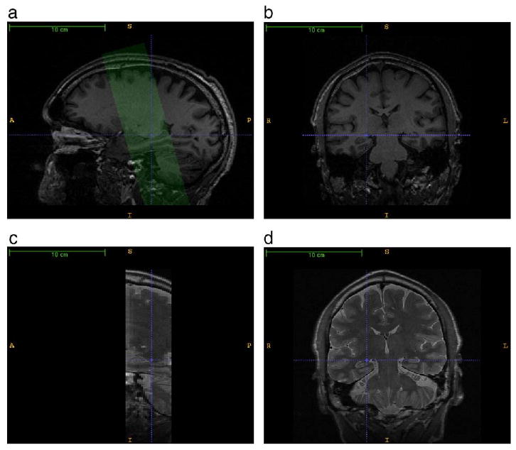
A comparison of the T1-weighted and T2-weighted MRI used by the automatic segmentation algorithm. a. A sagittal slice through the right hippocampal formation in the T1-weighted image. The green overlay illustrates the position and orientation of the T2-weighted image, which is oblique relative to the T1-weighted image. b. A coronal slice in the T1-weighted image; the dashed blue crosshairs point to the same voxel as in the sagittal slice. c. A sagittal slice through the T2-weighted image. d. A coronal slice through the T2-weighted image. The T2-weighted image offers greater contrast between hippocampal layers and greater in-slice resolution. In particular, a well-pronounced hypointense band formed by the innermost layers of the cornu Ammonis is apparent in both left and right hippocampi. However, the T2-weighted image has low resolution in the slice direction.

Perhaps the greatest advance towards automatic HF subfield segmentation was made recently by (Van Leemput et al., 2009), who used a statistical model with Markov random field priors to label HF subfields in “ultra-high resolution” T1-weighted MR images acquired with >35min acquisition time. Although this method clearly demonstrated the feasibility of automatic in vivo HF subfield segmentation, it has not yet been applied to MRI data that can be acquired with a short scan time.

HF Subfield Morphometry in Focal MRI: Manual Approaches

Some of the most exciting HF morphometry work uses what we call focal MRI sequences, which acquire a small number of thick slices with high in-plane resolution, slices that are oriented along the long axis of the HF, and relatively short scan time (see Figs. 1d and 2 for examples of such MRI). (Small et al., 2000) use a focal T2-weighted sequence to obtain high-resolution functional MRI of the HF and detect, based on manual delineation, subfield-level differences in MR signal between AD patients and controls. More recent functional MRI studies by (Zeineh et al., 2003; Suthana et al., 2009) use T2-weighted focal structural MRI to delineate boundaries between subfields and to study differences in functional activation across the HF; these authors unfold the HF, allowing effective visualization and more anatomically sensible processing of fMRI data. (Mueller and Weiner, 2009; Mueller et al., 2009; Wang et al., 2010; Malykhin et al., 2010) use focal T2-weighted MRI to estimate the volumes of hippocampal subfields based on a manual delineation protocol. In particular, (Mueller and Weiner, 2009) report cross-sectional volume differences between AD patients, MCI patients and controls that agree with patterns of atrophy known from pathology, i.e., significant reduction in CA1, subiculum and entorhinal cortex volume, and not in dentate gyrus or CA2 subfields.

Fig. 2.

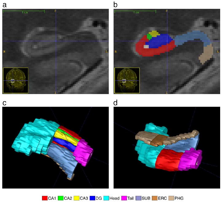
A close-up view of the right hippocampal formation in the image in Fig. 1. a. The coronal slice of the T2-weighted image, zoomed in by a factor of 10. b. Manual segmentation of the hippocampal formation overlaid on the coronal slice c,d. Three-dimensional rendering of the manual segmentation viewed from superior and inferior directions, respectively.

Despite the great promise of focal MRI for HF subfield morphometry and functional data analysis, we are not aware of any previous efforts to automate HF subfield segmentation in this kind of images.

Materials and Methods

Subjects

The imaging data for this study was collected by the Center for Imaging of Neurodegenerative Diseases (CIND) at the San Francisco Veterans Administration Medical Center. Our experiments use imaging data from 32 subjects, who participated in imaging studies at CIND. These subjects fall into three categories: control, mild cognitive impairment (MCI) of the AD type, and “cognitively impaired, non-demented (CIND).” Control (n=21) means cognitively intact control subject. Subjects in the MCI group (n=4) meet the diagnostic criteria in (Petersen et al., 1999) and also have a clinical diagnosis of MCI based on the consensus opinion of experienced neurologists. Subjects in the CIND group (n=7) have memory or executive deficits that are severe enough so that the referring clinicians suspected these subjects to be at risk for developing AD, but they do not fulfill the Research Criteria for MCI of the AD type or executive MCI. The subjects were between 38 and 82 years of age at the time of the scan, with average age 64.8±11.8 years. 18 subjects are male and 14 are female.

Imaging Protocol

All imaging was performed on a Bruker MedSpec 4 T system controlled by a Siemens Trio TM console using a USA instruments eight channel array coil that consisted of a separate transmit coil enclosing the eight receiver coils. The following sequences, which were part of a larger research imaging and spectroscopy protocol, were acquired: 1. 3D T1-weighted gradient echo MRI (MPRAGE) TR/TE/TI=2300/3/ 950 ms, 7° flip angle, 1.0×1.0×1.0 mm3 resolution, FOV 256×256×176, acquisition time 5.17 min, 2. high resolution T2 weighted fast spin echo sequence (TR/TE: 3990/21 ms, echo train length 15, 18.6 ms echo spacing, 149° flip angle, 100% oversampling in ky direction, 0.4×0.5 mm in plane resolution, 2 mm slice thickness, 24 interleaved slices without gap, acquisition time 3:23 min (adapted from (Vita et al., 2003; Thomas et al., 2004)), angulated perpendicular to the long axis of the hippocampal formation. Examples of T1 and T2-weighted images are shown in Figs. 1 and 2.

Manual Segmentation Protocol

The protocol for manual segmentation of the HF is derived from a published protocol (Mueller and Weiner, 2009), and expanded to include more coronal slices and additional subfields. ¹ Initially, each HF is partitioned into anterior (head), posterior (tail) and mid-region (body), with boundaries between these regions defined by a pair of adjacent slices in the MR image (i.e., each slice can contain only one label: head, tail, or body). The partitioning is based on heuristic rules. The hippocampal head is defined to start at the first slice where the uncal apex becomes visible, and extends anteriorly for approximately 6-7 slices. The hippocampal tail is defined by first identifying the wing of the ambient cistern. The slice immediately anterior to this was designated as tail, along with the three following slices in the posterior direction. The slices between head and tail slices are designated as hippocampal body.

The hippocampal head and tail are segmented as single structures because the “swiss roll” bends medially in these regions and develops additional folds (digitations of the head), causing severe partial volume effects and making differentiation between HF layers unreliable. The head label includes the anterior portion of the subiculum because it was not possible to separate these structures reliably. By contrast, in the hippocampal body, the “swiss roll” is roughly perpendicular to the slice plane, making subfield differentiation more feasible. Within slices designated as “body,” the hippocampal formation is divided into cornu Ammonis fields 1-3 (CA1-3), dentate gyrus (DG), subiculum (SUB) and a miscellaneous label, which contains cysts, arteries, etc. The subiculum is also traced in some of the “tail” slices because differentiation between hippocampus proper and the subiculum is possible there.

Additionally, the parahippocampal gyrus (PHG) is labeled, although this label is not constrained by the head/tail/body division and spans more slices than the other labels. The portion of the PGH belonging to the two most posterior “head” slices and the most anterior “body” slice is labeled as entorhinal cortex (ERC). The subdivision of the hippocampal slices into head/body/tail regions is illustrated in Fig. 3. An example of the manual segmentation is shown in Fig. 2.

Fig. 3.

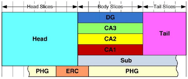
Diagram of the subdivision of the coronal slices in T2-weighted MRI into hippocampal head, body and tail. The vertical lines indicate coronal slices. The colored rectangles describe the subfields included in the manual segmentation protocol. Subfields CA1-3 and DG are defined in body slices; SUB is defined in body and tail slices; PHG is not restricted to specific slices, but the portion of the PHG belonging to three slices near the head-body boundary is designated ERC. The scale of the subfields in this diagram does not correspond to their actual volume.

Overview of the Automatic Segmentation Algorithm

We describe our approach as “nearly” automatic. This is because the partitioning of MRI slices into “body,” “head,” and “tail” is performed manually on the basis of two anatomical landmarks, as described in Section Manual Segmentation Protocol. Beyond this partitioning, the algorithm is fully automatic.

The segmentation algorithm assumes a set of N_train training images for which manual segmentations, which we treat as ground truth, are available, and a set of N_test test images that need to be segmented. Our algorithm consists of four steps.

1. An initial segmentation of the hippocampal subfields is generated for each training subject i using a multi-atlas segmentation technique, where the remaining N_train−1 datasets serve as atlases. Normalization to each of the atlases produces a candidate segmentation of subject i, and we combine these candidate segmentations into a single consensus segmentation using a voting scheme, as detailed in Multi-Atlas Segmentation and Voting (MASV). We call this algorithm multi-atlas segmentation and voting (MASV).

2. MASV results for the training subjects are compared to the corresponding manual segmentations, and voxels mislabeled by MASV are identified. AdaBoost classifiers are trained to detect such voxels (called bias detection, Section Bias Detection) and to assign the correct label to them (called bias correction, Section. Bias Correction). These classifiers use image texture, initial segmentation results, and spatial location as features.

3. An initial segmentation is obtained for each test subject using MASV. All N_train training subjects serve as atlases.

4. Classifiers trained in Step 2 are used to improve the initial segmentation of test subjects. Bias detection searches for mislabeled voxels in the initial segmentation, and bias correction assigns a new label to these voxels. The resulting labeling of the voxels is treated as the final segmentation of the test subjects.

Experiments in this paper are aimed at evaluating the accuracy of this four-step algorithm. Since manual segmentations are available for all the subjects in our dataset, we arbitrarily partition the dataset into training and test subsets. After obtaining the final segmentation of the test subset in Step 4 of the algorithm, we compare this final segmentation to manual segmentations of the test subset. As a means of cross-validation, we repeat this experiment for multiple random partitions of the dataset into training and test subsets.

The remainder of this Section describes in detail the two main components of this approach: the MASV framework and the bias correction/detection scheme.

Multi-Atlas Segmentation and Voting (MASV)

The multi-atlas approach to segmentation has become increasingly popular in the recent years, thanks in part to new inexpensive parallel computing environments (Rohlfing et al., 2004; Klein and Hirsch, 2005; Chou et al., 2008; Aljabar et al., 2009; Artaechevarria et al., 2009; Collins and Pruessner, 2009). In this approach, registration is used to normalize a target image to multiple template images, each of which has been segmented manually. Manual segmentations from template images are warped into the space of the target image and combined into a consensus segmentation using a voting scheme. The multi-atlas approach tends to be more accurate than when a single template is used. Our “MASV” approach uses the same idea, adapting it as is necessary to the specificities of focal T2-weighted MRI data.

In each subject, we use both T1 and focal T2-weighted MRI because these images provide complementary information. Focal T2-weighted images have high in-plane resolution and good contrast between subfields, but these images also have a limited field of view and large slice spacing. On the other hand, the T1-weighted images have nearly isotropic voxels and cover the entire brain, but lack contrast between subfields. MASV aims to normalize the hippocampal formation between each subject and each atlas using a combination of data from both modalities. The following steps are involved in the MASV approach:

1. Within-subject rigid alignment of T1 and T2 data. This corrects for subject motion between T1 and T2 scans. This and the following two steps are performed for all subjects in the study, regardless of whether they are treated as atlases or as images to be segmented.

2. Deformable registration of the T1 images to a T1-weighted population template. This registration factors out much of the anatomical difference between the subjects and brings all subjects into a common space for subsequent analysis. In each hemisphere, a region of interest surrounding the HF is defined.

3. Cropping of the image region surrounding the hippocampal formation in T1 and T2 images and resampling to a common isotropic 0.4×0.4×0.4mm³ voxel grid. This step makes subsequent registration more efficient and accounts for differences in voxel size between T1 and T2 data.

4. Pairwise registration between the target subject and multiple atlases using multi-modality (T1 and T2) image matching.

5. Consensus segmentation using similarity-weighted voting.

This pipeline is implemented using freely available tools FSL/FLIRT, ANTS, and Convert3D. We will now describe each step in more detail.

Within-Subject Rigid Alignment

The FSL/FLIRT global image registration tool (Smith et al., 2004) is used to align each subject's T2 image to the T1 image. The initial alignment is given by the DICOM image headers, but subject motion between the scans can result in a slight misalignment. We use the normalized mutual information metric (Studholme et al., 1997) to account for differences in image modality. FLIRT is run with six degrees of freedom, allowing for rigid motion. In a few images, strong intensity features in the skull tend to throw registration off; i.e., the skull in T2 image is matched to the CSF in the T1 image. To prevent this from happening, we crop the T2 images by 40% in the in-plane dimension, effectively removing the skull and part of the brain far away from the hippocampus.

Deformable Registration to a Population-Specific Template

The T1 images of all subjects in the study are normalized to a population-specific template using the open-source deformable registration tool ANTS. The Symmetric Normalization (SyN) algorithm implemented by ANTS is described in (Avants et al., 2008). SyN was found to be one of top two performers in a recent evaluation study of 14 open-source deformable registration algorithms by (Klein et al., 2009). SyN uses a diffeomorphic transformation model and supports a variety of image match metrics. ANTS provides functionality for generating optimal templates, given a collection of images. Such optimal templates have been recognized to offer advantages over a priori templates for image normalization (Guimond et al., 2000; Joshi et al., 2004; Avants et al., 2009). Building a template involves iteratively registering images to the current template estimate; computing a new shape and intensity average from the results of these registrations; and setting the current template estimate to be that average. This procedure is repeated until the template estimate converges. Each registration in this procedure uses SyN with default parameters and the cross-correlation image match metric.

Resampling to a Hippocampal Reference Space

The T1 template is used to define a reference space in which all subsequent processing takes place. A separate reference space is defined for the left and right hippocampi. The reference space is a rectangular region of the T1 template surrounding one of the hippocampi and resampled to have voxel size 0.4×0.4×0.4 mm³. The dimensions of the reference space are 40×55×40 mm³, with the longest dimension along the anterior-posterior axis. The reference space includes the hippocampus formation, parahippocampal gyrus, amygdala, temporal horn of the lateral ventricle, and other surrounding structures. The reference space is illustrated in Fig. 4.

Fig. 4.

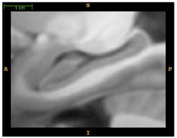
A sagittal slice of the reference space extracted from the T1 population template. This image is the average of 32 subject T1-weighted images warped to the template space and resampled at 0.4 mm isotropic resolution.

All T1 and T2 subject images are warped and resampled into the reference space. Subsequent subject-to-subject registrations are performed on these resampled images. The reason for doing so is that the initial normalization to the T1 template removes much of the variability in the shape of the hippocampal regions between subjects. Subsequent subject-to-subject registrations must only account for residual misregistration and are thus more tractable and less prone to falling into local optima than the alternative of registering subject images to each other directly.

Within the reference space, a mask is defined by manually segmenting the hippocampus and dilating the segmentation by a spherical structural element with the radius of 10 cm. This mask helps further speed up subsequent registrations, and prevents the boundaries of the reference space from influencing the registration. The shape of the mask can be seen in Fig. 5, second row.

Fig. 5.

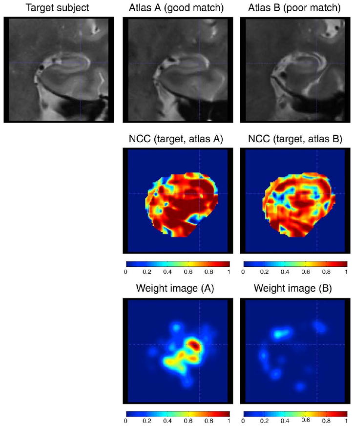
Illustration of the similarity-weighted voting procedure. Top row: coronal slice from the target T2-weighted image warped to the reference space, and coronal slices from two “atlases” warped to the target image using deformable registration. Middle row: Maps of normalized cross-correlation (C_i,j in the text) between the target image and warped atlas images. The binary mask used during registration is applied to the cross-correlation images. Bottom row: weight images (W_i,j) derived for each atlas by ranking the cross-correlation maps, applying an inverse exponential, and smoothing (see text for details). Larger weight values should indicate greater similarity between the atlas and the target image. Atlas A is better registered to the target image than Atlas B, so the cross-correlation map and weight image for Atlas A have greater values than for Atlas B. Continued in Fig. 6.

Subject-to-Subject Multimodality Registration

The most computationally intensive component of the initial segmentation algorithm is the multi-modality registration between each subject and each atlas. There are (N_train−1) N_train such registrations in the training stage of the algorithm (Step 1 in Section. Overview of the Automatic Segmentation Algorithm) and N_test N_train registrations in the testing stage (Step 3 in Section. Overview of the Automatic Segmentation Algorithm) ². Each registration is performed using the SyN algorithm. The image match metric is the average of the cross-correlation between T1 images and cross-correlation between T2 images. Cross-correlation at each voxel is computed using a 9×9×9 voxel window. ³ Registration is performed ina multi-resolution scheme, with a maximum of 120 iterations at 4× subsampling, 120 iterations at 2×subsampling, and 40 iterations at full resolution. The mask created in the template space is used to reduce the number of voxels where the metric is computed. Each registration ran for under one hour on a 2.8 GHz CPU.

Consensus Segmentation using Metric-Weighted Voting

For clarity, in this subsection we call the subject for whom we wish to obtain a segmentation the target subject. The target subject may be part of the training set or test set, depending on the stage of the algorithm, as discussed above in Section. Overview of the Automatic Segmentation Algorithm. By warping each of the atlas segmentations into the space of the targets subject's T2 image, we can produce a set of m candidate segmentations of the target subject. The challenge is to combine these different candidate segmentations into a single consensus segmentation. Several schemes for combining segmentations have been proposed, , such as majority voting (Heckemann et al., 2006), similarity-weighted voting (Artaechevarria et al., 2009; Collins and Pruessner, 2009) and STAPLE (Warfield et al., 2004), the latter primarily intended for combining manual segmentations from raters who differ in expertise. In our work, we adopt a weighted voting scheme, where the contribution from each training segmentation is weighted locally by the image match between the T2 image of the target subject and the T2 image of the training subject. The scheme is local because voting occurs independently at each voxel. Our choice of similarity-weighted voting is motivated by the observation that many of the target-to-atlas registrations fail to align anatomical structures properly, probably due to falling into a local optimum. Similarity-weighted voting helps us assign larger weight to the atlases that registered better to the target subject. Since we use free-form registration, it is possible that an atlas matches a target subject well in one part of the image and does so poorly inother parts of the image. Voxel-wise voting helps account for this spatial variability in registration accuracy.

Let M_k be the rigid transformation from the T2 image to the T1 image for subject k, let ψ_k be the deformable transformation from the T1 image of subject k to the reference space, and let χ_ij be the deformable transformation computed by subject-to-subject multi-modality registration between target subject i and atlas j. In the reference space, we compute the cross-correlation between the warped target T2 image ψ_i ∘M_i ∘ $I_i^{\text{T}2}$ and the warped atlas T2 image χ_ij ∘ψ_j ∘M_j ∘ $I_j^{\text{T}2}$. Cross-correlation is computed at each voxel, producing an image, which we denote C_i,j. Higher values of cross-correlation indicate better texture match between the two registered images, as Fig. 5 illustrates. Taking all such images C_{i, 1} …C_i, N_train for the target subject i, we perform voxelwise ranking, producing a new set of rank images R_{i, j}:

$$R_{i,j}(\mathbf{\text{x}})=\left|\left\{p:C_{i,p}(\mathbf{\text{x}})>C_{i,j}(\mathbf{\text{x}})\right\}\right|.$$

These rank images are converted into weight images by applying the inverse exponential function and smoothing spatially with an isotropic Gaussian filter:

$$W_{i,j}(\mathbf{\text{x}})=G_{\sigma }\circ e^{-\alpha R_{i,j}(\mathbf{\text{x}})},$$ (1)

where α>0 is a constant weighting factor and σ is the standard deviation of the Gaussian. Under the inverse exponential mapping, the training subject that best matches the target subject at voxel x is assigned weight 1, the training subject with second-best match is given weight e^−α and so on. These weight images are used to compute a consensus segmentation of the target subject as the weighted sum of the atlas-based segmentations. Specifically, let be the set of all segmentation labels, plus the background (null) label. Let ${\mathit{\text{I}}}_j^l$ be a binary image in the native space of the training image j, with ${\mathit{\text{I}}}_j^l=1$ at voxels that are assigned label l∈ and ${\mathit{\text{I}}}_j^l=0$ at all other voxels. Using these binary label images and the weight images from above, we compute label density maps, in template space, for the target subject i as follows:

$${\mathit{\text{D}}}_i^l(\mathbf{\text{x}})=\frac{1}{Z}\sum _{j=1}^{N_{\text{train}}}{W}_{i,j}(\mathbf{\text{x}}){\mathit{\text{I}}}_j^l(M_j^{-1}({\psi }_j^{-1}({\chi }_{ij}^{-1}(\mathbf{\text{x}})))),$$ (2)

where $Z={\sum }_{j=0}^{N_{\mathit{\text{train}}}-1}{e}^{-\alpha j}$ is a normalizing constant. ⁴ These density maps are illustrated in Fig. 6.

Fig. 6.

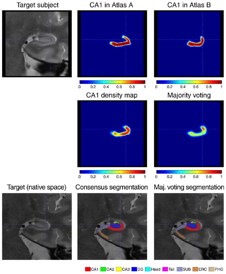
Illustration of the similarity-weighted voting procedure (continued from Fig. 5). Top row: CA1 segmentations from atlases A and B warped to the target image. Middle row, left: CA1 density map ( ${\mathit{\text{D}}}_i^l$ in the text) computed as the weighted sum of warped CA1 segmentations from all atlases (weights W_i,j illustrated in Fig. 5). Middle row, right: density map computed using simple majority voting, i.e., equal weight averaging of warped labels from all atlases. The density map produced using weighted voting has greater density throughout CA1. Bottom Row: coronal slice in the target image, in its native image space, with overlaid consensus segmentations produced using similarity-weighted and majority voting. The consensus segmentation is the final output of MASV.

Density maps computed using (2) do not take into account the rules defined in the segmentation protocol, e.g., that CA1-3 must lie inside the slices designated as hippocampal body, and so on (see Section Manual Segmentation Protocol and Fig. 3). To incorporate these rules we derive augmented density maps ${\stackrel{\sim }{D}}_i^l(\mathbf{\text{x}})$, in native space of target subject i, as follows:

$${\stackrel{\sim }{D}}_i^l(\mathbf{\text{x}})={\stackrel{\sim }{D}}_i^l(x,y,z)=\{\begin{array}{ll}{\mathit{\text{D}}}_i^l({\psi }_i(M_i(x,y,z)))& \text{if label}l\text{may occur in slice}z\\ 0& \text{otherwise}\end{array}$$

From these augmented native-space density maps, a consensus segmentation is computed by choosing at each voxel the label with the largest density:

$${\overline{S}}_i(\mathbf{\text{x}}){=}_{l\in \mathcal{\text{ℒ}}}^{\mathit{\text{arg max}}}{\stackrel{\sim }{D}}_i^l(\mathbf{\text{x}}).$$

An example of consensus segmentation is shown in Fig. 6.

The behavior of this voting scheme is controlled by two parameters: α and σ. Larger values of α lead to greater bias in favor of the atlases that best match the target image at a voxel. For example, if α=1, the weight assigned to the atlas with the best match to the target image (at a given voxel) is greater than the sum of the weights assigned to all other atlases (i.e., $e^0>{\sum }_{a=1}^{N_{\mathit{\text{atlas}}}}{e}^{-a}$). That means that the consensus segmentation ignores all segmentations except the one coming from the best matching atlas. On the other hand, if α=0, all atlases are assigned the same weight, regardless of similarity to the target image. This is known as simple majority voting.

Parameter σ controls the degree of spatial regularization during the computation of weight images W_{i, j}. When σ=0, voting is done completely independently at each voxel. When σ>0, atlas-target similarity in the neighborhood of a voxel affects the voting weights at that voxel. In the extreme case, when σ→∞, the voting is no longer spatially varying, i.e. each atlas is assigned a single weight based on its overall similarity to the target image.

In our experiments we set a priori parameter values α=1 and σ=1.2mm. We perform post hoc testing to evaluate the sensitivity of segmentation outcome to these two parameters.

Segmentation Refinement via AdaBoost Learning

The initial segmentations produced using MASV are further refined using a machine learning technique. The flowchart of this approach is given in Fig. 7. As summarized in Section. Overview of the Automatic Segmentation Algorithm, MASV is applied both to training and test datasets. In the training set, initial segmentations produced by MASV are compared to the ground truth manual segmentations, and voxels mislabeled by MASV are identified. An AdaBoost classifier is trained to recognize such mislabeled voxels. We refer to this classifier as bias detection, because it is capable of detecting systematic biases in the initial segmentation relative to the ground truth. ⁵ A second kind of AdaBoost classifier is trained to assign the correct label to each of the voxels flagged as mislabeled by bias detection. We refer to this type of classifier as bias correction. Bias detection and bias correction are applied to the results of the initial segmentation in the test dataset to obtain the final segmentation. We now describe bias correction and bias detection in greater detail.

Fig. 7.

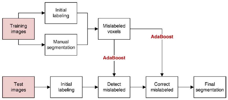
Flowchart of the segmentation refinement algorithm. In the training set, initial segmentation results from MASV are compared to ground truth manual segmentations, and a classifier is trained to recognize mislabeled voxels. Additionally, classifiers are trained to assign the correct label to each mislabeled voxel. MASV is also applied to images in the test set. Its results are refined by using the first type of classifier to detect voxels mislabeled by MASV and by using the second type of classifier to assign a correct label to these voxels.

Bias Detection

The task of bias detection is to identify voxels wrongly labeled by the initial segmentation algorithm. This is a binary classification problem: a voxel in the T2 image is either correctly labeled or wrongly labeled. We use the AdaBoost algorithm (Freund and Schapire, 1995) to iteratively build a strong classifier by combining complementary weak classifiers derived from a rich feature pool. Informally, two classifiers are complementary to each other if they do not make similar mistakes. At each voxel in the T2 image, three types of features are obtained: appearance features, contextual features and spatial features. We denote A^Δx,Δy,Δz(P)= I(P_x + Δx, P_y + Δy, P_z + Δz)–Ī to be the appearance feature at the relative location (Δx,Δy,Δz) for voxel P with coordinates (P_x,P_y,P_z). I is intensity of the T2-weighted image. To compensate for different intensity ranges, we normalize the intensities by the average intensity of the hippocampus region of interest, Ī. Besides the intensity features, we use subfield labels from the initial segmentation as contextual features, similarly to Morra et al. (2009a). We denote the contextual feature as L^Δx,Δy,Δz(P) = S̄ (P_x + Δx, P_y + Δy, P_z + Δz), where S̄ is the result of the initial subfield segmentation. To include spatial information, we use Q_x(P) = P_x–x̄, Q_y(P) = P_y–ȳ and Q_z(P) = P_z–z̄, where x̄ is the center of mass of all the subfields combined, computed from the initial segmentation. To enhance the spatial correlation of our features, we include the joint feature obtained from multiplying the spatial feature with the appearance and contextual features. For example, the joint features of appearance and location include A^{Δx, Δy, Δz}(P)Q_x(P), A^{Δx, Δy,Δz}(P)Q_y(P), and A^Δx,Δy,Δz(P)Q_z(P). Since the in-slice resolution of T2-weighted images is much higher than slice thickness, we use – 6≤Δx, Δy ≤6 and Δz=0. Overall, we use ∼ 1300 features to describe each voxel.

For each feature in the feature set, a weak classifier is constructed by selecting an optimal threshold to identify mislabeled voxels. AdaBoost is then used to iteratively select weak classifiers based on their ability to correctly classify “difficult” training cases, meaning those cases that are poorly classified by previously selected weak learners. The final strong classifier is a weighted sum of the weak classifiers.

Bias Correction

Bias detection outputs candidate voxels that we suspect to be mislabeled in the initial segmentation. We then need to reassign new, hopefully correct, labels to them. There are many ways to approach this problem. One simple method is to enforce the correct topology of subfields. For instance, if a voxel at the boundary of CA1 and DG is mislabeled, and its neighbor voxels are correctly labeled, because of the topology constraints, we know that the correct label for this voxel has to be either CA1 or DG. Hence, switching its label can correct it. This simple method can correct most mislabeled voxels, however it may run into trouble at 3-way or 4-way boundaries. For a more robust method, again we use a learning-based method. Given all the voxels that are mislabeled in the initial segmentation, we train classifiers to map them to the correct labels. This is a multi-class classification problem. We follow the common practice and train a binary classifier for each label to separate it from other labels. For this task, we use AdaBoost training with the same set of features as described above. Since we only use the mislabeled data for training, the learning cost is much less than that using the entire training data. Moreover, by not taking the correctly labeled voxels into consideration, relabeling the mislabeled voxels is a simpler problem than relabeling the whole hippocampus, which simplifies the learning step as well. After bias detection, we reevaluate each detected mislabeled voxel by each classifier and assign the label whose corresponding classifier gives the highest score to the voxel.

Evaluation of Segmentation Accuracy

Evaluation is performed by comparing automatic segmentation results to manual segmentations. As a way of bootstrapping, we perform N_exp=10 cross-validation experiments, each using N_train= 21 randomly selected training images and N_test=10 test images. In each of these experiments, manual segmentations by JP are used as training, because they are available for both hemispheres in the entire set of subjects.

When reporting results, we primarily compare segmentations generated on the test data to the manual segmentations by JP. However, during the evaluation of our manual segmentation protocol, a subset of N_rel=10 images was segmented twice by two raters (JP and CC) to establish reliability. Within each cross-validation experiment, a subset of these reliability images is included among the test images (e.g., in the first of 10 cross-validation experiments, 4 out of 10 test subjects have been segmented by both CC and JP). For this subset, we compute Dice overlap between the automatic segmentation and manual segmentations by both raters. Averaging over all the cross-validation experiments, we obtain an estimate of segmentation accuracy across different raters. Thus, in the Results section, we list two sets of comparisons: automatic method compared to JP on a larger set of test subjects, and automatic method compared to both raters on a smaller set of test subjects.

When comparing automatic and manual segmentations, we employ several complementary metrics. We measure relative volumetric overlap between two binary segmentations using the Dice similarity coefficient (DSC) (Dice, 1945). DSC between two segmentations (i.e., sets of voxels) A and B is given by

$$\text{DSC}(A,B)=\frac{\left|A\cap B\right|}{\frac{1}{2}\left(\left|A\right|+\left|B\right|\right)}.$$

We compute and report Dice overlap separately for each subfield.

Boundary displacement error (BDE)

Is measured as root mean squared distance between the boundaries of two binary segmentations. It is computed by extracting a dense triangle mesh representation of the boundary of each segmentation. Given two such meshes, and , this error is given by

$$\text{BDE}(A,B)={\left[\frac{1}{2}\sum _{v\in V_A}d{(v,\mathcal{\text{B}})}^2+\frac{1}{2}\sum _{v\in V_{\mathcal{\text{B}}}}d{(v,\mathcal{\text{A}})}^2\right]}^{\frac{1}{2}},$$

where V denotes the set of vertices in the mesh , and d(v, ) denotes Euclidean distance from vertex v to the closest point (not necessarily a vertex) on the mesh Like overlap, boundary displacement error is computed and reported separately for each subfield. Overlap and boundary displacement measures are highly complementary because the former measures relative segmentation error and the latter measures absolute segmentation error.

Additional metrics used in this paper include subfield volume and overall segmentation error. Subfield volume is simply measured by adding up voxels in a segmentation and multiplying by the volume of the voxel. Overall segmentation error is used as a summary measure of segmentation accuracy across all subfields. It is computed between a test segmentation (e.g., automatic segmentation) and a reference segmentation (e.g., manual segmentation) and given by

$$\text{OSE}(T,R)=\frac{\left|\left\{i:T_i\ne R_i\right\}\right|}{\left|R\right|},$$

where T_i denotes the label assigned to voxel i in the segmentation T. We use the overall segmentation error when reporting the results of post hoc parameter tuning experiments, where a summary measure of segmentation accuracy is needed.

Results

Comparison to Manual Segmentation by Primary Rater (JP)

To evaluate segmentation accuracy, we compare automatic segmentation results to manual segmentations. Fig. 8 shows examples of automatic and manual segmentation in three arbitrarily chosen subjects from the first of ten cross-validation experiments. Intermediate results of MASV and bias detection are also illustrated.

Fig. 8.

Examples of automatic and manual segmentations in three target subjects. Left HF is shown in subjects 1 and 3; right HF is shown in subject 2. Shown from left to right are (1) detail of the coronal slice of the T2-weighted image (in native image space); (2) result of multi-atlas segmentation with similarity-weighted voting (MASV); (3) voxels declared “mislabeled” by the learning-based bias detection algorithm; (4) final segmentation, after applying learning-based bias correction to relabel “mislabeled” voxels; (5) manual segmentation.

Average Dice overlap between the automatic segmentation and manual segmentation by rater JP is given for each subfield in the first column of Table 1. The averages are taken over N_exp=10 cross-validation experiments and within each experiment, over N_test=10 segmentations. The overlaps for left and right hippocampi are included in the averages. Thus, each entry in Table 1 is an average of 2·N_exp·N_test=200 pairwise automatic-manual comparisons. The average Dice overlap for larger subfields (CA1, DG) as well as head and tail regions, exceeds 0.85. For smaller subfields (CA2, CA3), overlap is substantially lower, just above 0.5. For SUB and ERC, overlap exceeds 0.75.

Table 1.

A comparison of the accuracy of three variants of the automatic segmentation algorithm. The first variant is the algorithm as described in the paper. The second variant is the algorithm without the AdaBoost learning step, i.e., just the initial segmentation. The third variant is initial segmentation implemented with simple majority voting in place of similarity-weighted voting. For each variant, the mean ± standard deviation of the Dice overlap between the automatic segmentation and manual segmentation by JP is given. The statistics are computed over 10 cross-validation experiments with 10 test datasets in each experiments. Left and right hemispheres are pooled in the statistics.

Subfield	Accuracy (Dice Overlap) by Variant of Automatic Method
	Full Method (MASV+AdaBoost)	MASV Only	MASV with Majority Voting
CA1	0.875 ± 0.033	0.851 ± 0.040	0.804 ± 0.059
CA2	0.538 ± 0.171	0.470 ± 0.179	0.357 ± 0.194
CA3	0.618 ± 0.128	0.583 ± 0.133	0.530 ± 0.145
DG	0.873 ± 0.042	0.859 ± 0.045	0.813 ± 0.087
HEAD	0.902 ± 0.018	0.893 ± 0.018	0.878 ± 0.021
TAIL	0.863 ± 0.093	0.828 ± 0.105	0.793 ± 0.112
SUB	0.770 ± 0.061	0.742 ± 0.063	0.715 ± 0.062
ERC	0.787 ± 0.097	0.738 ± 0.093	0.696 ± 0.108
PHG	0.706 ± 0.064	0.658 ± 0.073	0.627 ± 0.074

To illustrate the effect of the main components of the proposed segmentation method, Table 1 also lists average overlap for two variants of the method. In the first variant (column 2), the initial segmentation using MASV is performed, but AdaBoost bias detection and correction are not performed. In the second variant (column 3), the MASV is performed using simple majority voting instead of the similarity-weighted voting described in Section Consensus Segmentation using Metric-Weighted Voting, and AdaBoost is not used. Across all subfields, the full method performs better than MASV, and MASV with similarity-weighted voting performs better than simple majority voting. The improvements due to weighted voting are substantial, particularly for small subfields (e.g., 0.11 increase in overlap for CA2). The improvements due to AdaBoost range from as much as 0.06 for CA2 to as little as 0.01 for HEAD, and are generally greater for smaller, harder to segment structures.

Table 2 compares the performance of the three variants based on the boundary displacement error metric. Again, a similar pattern of consistent improvement due to bias correction and similarity-weighted voting is observed in all subfields. Subfields CA1 and DG, which have Dice overlap over 0.87, also have RMS boundary displacement error below the in-slice voxel size (0.4 mm). Small subfields CA2 and CA3, where the Dice overlap is lowest among all subfields, have relatively small boundary errors, close to the in-slice voxel size. ERC, another relatively small subfield, does fairly well in terms of both metrics, with 0.79 overlap and 0.44 mm boundary error. On the other hand, large subfields HEAD and TAIL, which have very high Dice overlap, do much worse in terms of boundary displacement. Subfields SUB and PHG perform worst in terms of displacement errors. These are also the only two subfields for which the rules defined in the segmentation protocol do not explicitly specify the starting and ending slices (see Section Manual Segmentation Protocol and Fig. 3).

Table 2.

A comparison of the accuracy of three variants of the automatic segmentation algorithm in terms of boundary displacement error. The columns are defined in the caption to Table 1.

Subfield	Boundary Displacement Error (mm) by Method Variant
	Full Method (MASV+AdaBoost)	MASV Only	MASV with Majority Voting
CA1	0.282 ± 0.079	0.320 ± 0.090	0.412 ± 0.139
CA2	0.411 ± 0.308	0.480 ± 0.342	0.640 ± 0.563
CA3	0.395 ± 0.279	0.432 ± 0.287	0.501 ± 0.406
DG	0.287 ± 0.124	0.318± 0.139	0.424 ± 0.232
HEAD	0.594 ± 0.092	0.623 ± 0.093	0.693 ± 0.105
TAIL	0.572 ± 0.394	0.636 ± 0.446	0.728 ± 0.468
SUB	0.639 ± 0.272	0.675 ± 0.275	0.697 ± 0.247
ERC	0.443 ± 0.216	0.497 ± 0.209	0.566 ± 0.246
PHG	0.803 ± 0.273	0.856 ± 0.262	0.880 ± 0.238

Comparison to Manual Segmentation by Two Raters

A subset of N_rel=10 images in our dataset was used for the reliability analysis of manual segmentation. The left and right hippocampal formations were segmented by raters JP and CC in these images. In this subset of images, we compare the performance of the automatic segmentation against rater JP (whose segmentations were used to train the method) to the performance against rater CC, whose segmentations were not used for training. These comparisons, in terms of average Dice overlap, are given in the first two columns of Table 3.The Dice overlapisaveraged over 68hippocampal formations, because 34 of the N_exp ·N_test=100 test images belong to the subset of N_rel images used for reliability analysis. ⁶ Overall, overlap between the automatic method and individual raters is relatively close to the average inter-rater overlap for each subfield but substantially lower than the average intra-rater overlap. When comparing the automatic method to both raters, we do not observe a consistent bias towards JP even though JP produced the segmentations on which the automatic method was trained. Only for one of the subfields, CA1, the bias approaches significance (p=0.052) ⁷.

Table 3.

Agreement between automatic and manual segmentations by two raters. The columns describe five comparisons: automatic method vs. rater JP, whose manual segmentations were used to train the automatic method; automatic method vs. rater CC, whose manual segmentations were not used for training; rater JP vs. rater CC; and average intra-rater agreement for raters JP and CC. Agreement is reported as Dice overlap (mean ± standard deviation). Human rater agreement values are averages over 10 images from the dataset for which segmentations by both raters are available (10 left and 10 right hippocampi). The comparisons of automatic method vs. human rater use the same 10 images, but are also averaged over the 10 cross-validation experiments (note that only a subset of these 10 images form part of the “test” set in each cross-validation experiment, so overall, human vs. automatic results are averages over 68 (34 left + 34 right) automatic segmentation attempts). Note that the difference between the first column in Table 3 and the first column in Table 3 is only the set of subjects (all vs. 10) over which automatic-to-manual agreement is averaged.

	Auto vs. JP	Auto vs. CC	JP vs. CC	JP vs. JP	CC vs. CC
CA1	0.883 ± 0.029	0.876 ± 0.039	0.883 ± 0.032	0.921 ± 0.010	0.919 ± 0.017
CA2	0.533 ± 0.162	0.503 ± 0.162	0.522 ± 0.160	0.730 ± 0.108	0.737 ± 0.095
CA3	0.624 ± 0.076	0.603 ± 0.071	0.668 ± 0.087	0.814 ± 0.072	0.772 ± 0.103
DG	0.890 ± 0.022	0.889 ± 0.034	0.885 ± 0.034	0.931 ± 0.015	0.922 ± 0.023
HEAD	0.893 ± 0.016	0.897 ± 0.016	0.900 ± 0.016	0.934 ± 0.015	0.950 ± 0.017
TAIL	0.865 ± 0.078	0.861 ± 0.104	0.901 ± 0.059	0.927 ± 0.023	0.956 ± 0.016
SUB	0.777 ± 0.044	0.786 ± 0.049	0.768 ± 0.079	0.882 ± 0.033	0.910 ± 0.024
ERC	0.794 ± 0.126	0.771 ± 0.147	0.786 ± 0.123	0.856 ± 0.077	0.894 ± 0.028
PHG	0.710 ± 0.050	0.692 ± 0.067	0.706 ± 0.106	0.860 ± 0.025	0.876 ± 0.028

Reliability of Subfield Volume Estimation

Measures of volume overlap and boundary displacement error reflect how well the proposed algorithm localizes subfields in MR images. However, for cross-sectional analysis, it is also important to show that the volume estimates produced by automatic and manual segmentation are consistent. Fig. 9 shows Bland-Altman plots comparing automatically estimated subfield volume to the volume estimated manually. The volumes are highly correlated for CA1, DG and Head subfields, with less correlation for smaller subfields. Fig. 10 plots the intraclass correlation coefficient (ICC) (Shrout and Fleiss, 1979) expressing agreement between automatic segmentation and manual segmentation by rater JP. We use the variant of ICC that (Shrout and Fleiss, 1979) call ICC(2,1), which measures absolute agreement between volume measurements under a two-way random ANOVA model. In Fig. 10, ICC is computed separately for each cross-validation experiment, and a box-whisker plot is used to display the range of ICC values for each subfield. ICC is relatively large for subfields CA1 (average over 10 cross-validation experiments is 0.89) , DG (0.94) and HEAD (0.91). It is substantially lower, with average in the range 0.4-0.5 for CA2, CA3, ERC, SUB and TAIL. For PHG the ICC is particularly low (0.19), which may be explained by the fact that it's extent in the slice direction is not constrained by heuristic rules, as for the other subfields.

Fig. 9.

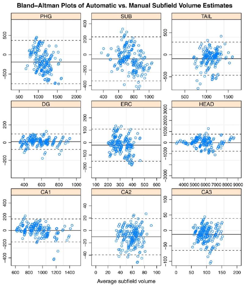
Bland-Altman plots comparing automatic volume estimates to manual volume estimates by rater JP for each subfield. Each point corresponds to a segmentation of one of the two hemispheres in one of N_test test subjects in one of the N_exp cross-validation experiments. The difference between automatic and manual estimates is plotted against their average. The solid horizontal line corresponds to the average difference, and the dashed lines are plotted at average ±1.96 standard deviations of the difference.

Fig. 10.

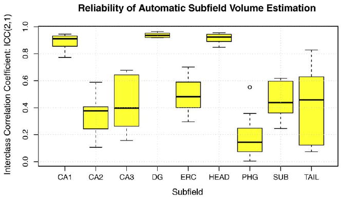
Agreement between automatically and manually derived estimates of hippocampal subfield volume. For each subfield, the box-whisker plot shows the range of ICC coefficients obtained from 10 cross-validation experiments (‘boxes’ are drawn between lower and upper quartiles; 'whiskers' indicate minimum and maximum values, minus the outliers, indicated by circles; the bold line represents the median). Large values of ICC indicate better agreement. See text for details.

Post hoc analysis of voting parameters

As discussed in Section. Consensus Segmentation using Metric-Weighted Voting, the similarity-weighted voting scheme is controlled by two parameters: the bias parameter α and the regularization parameter σ. In the experiments above, these parameters were set to a priori values α=1, σ=1.2mm. To determine how sensitive segmentation results are to these parameters, we perform post hoc analysis. This analysis performs multi-atlas segmentation and voting using different values of α and σ for a single random partition of the data set into 22 atlases and 10 target images. Bias detection/correction is not performed. For each subject, we measure the overall segmentation error (OSE), described in Section 3.7. Figs. 11 and 12 plot segmentation error against α and σ, respectively. Interestingly, our a priori choice of parameter values was fairly effective. Indeed, α=1 results in lowest segmentation error, and with respect to σ, segmentation error reaches lowest values in the range 1-1.4 mm.

Fig. 11.

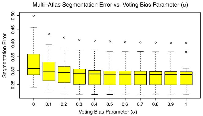
Segmentation error vs. voting bias parameter α.

Fig. 12.

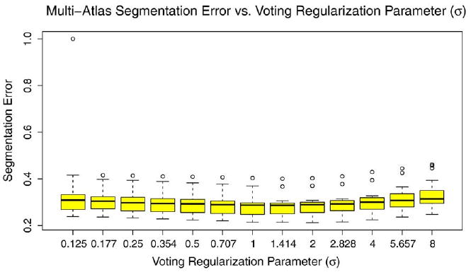
Segmentation error vs. voting regularization parameter σ.

Discussion

We have presented a technique that allows hippocampal subfields to be segmented automatically with a relatively small amount of input from a human expert. The accuracy of our technique, measured in terms of Dice overlap, is very close to inter-rater reliability for manual segmentation. For larger subfields, including CA1 and DG, there is high (≈0.9) intraclass correlation between manually and automatically measured hippocampal volumes, which suggests that the automatic method may be used in place of manual segmentation for cross-sectional analysis of subfield volume changes due to various brain disorders. In the following sections, we compare our results to previously published results, discuss the limitations and potential improvements to our approach, and discuss how our approach can be leveraged in future studies.

Comparative Evaluation and Significance of the Results

This work is most closely related to the hippocampus subfield segmentation paper by (Van Leemput et al., 2009). As we note in the Background section, the two techniques are applied to very different MRI data, which complicates a direct comparison of the results. (Van Leemput et al., 2009) acquire multiple averages over a 35 min scan time to obtain high-contrast T1-weighted images with 0.4 × 0.4 × 0.8mm³ resolution. By contrast, we use a sequence with acquisition time is under 4 min to obtain data that has 0.4 × 0.5 × 2.0mm³ resolution and T2 weighting. The resulting images have a distinct hypointense band between layers of the HF, but they suffer from severe partial voluming. The differences between the two approaches also extend to the anatomical definition of HF subfields. (Van Leemput et al., 2009) primarily list geometrical rules as criteria for defining subfields, whereas the protocol used in this paper generally proceeded by comparing in vivo image slices to annotated postmortem data in published atlases, such as (Duvernoy, 2005), although geometric rules are used for defining the boundaries of smaller subfields CA2 and CA3. Visually, HF subfield definitions in our work are very different from ((Van Leemput et al., 2009), Fig. 1). In terms of methodology, there are similarities between (Van Leemput et al., 2009) and our work. Both methods use example segmentations to train the automatic method. Van Leemput et al. frame the segmentation problem in Bayesian terms and use a tetrahedral mesh model to represent the hippocampal formation, whereas our work relies on deformable image registration and machine learning. The Dice overlaps reported in our paper are generally higher than those reported by(Van Leemputetal.,2009).We report overlap above 0.85 for CA1, DG, HEAD and TAIL, and overlap above 0.75 for ERC and SUB, whereas the highest overlap reported for any subfield by (Van Leemput et al., 2009) is around 0.75. However, a direct comparison of overlap values between the two papers should be read with a great deal of caution, given the differences in anatomical definition of subfields, and due to the fact that head/body/tail slice boundaries are supplied as manual input to our method.

One of the highly encouraging outcomes of this study is that the segmentation accuracy for subfields CA1 and DG is comparable to some of the best results published for whole-hippocampus automatic segmentation. There is a wide range of variability in whole-hippocampus segmentation results reported in the literature. ((Colollins and Pruessner, 2009), Table 1) give a comprehensive listing of automatic segmentation results reported in the last ten years. Dice overlap between automatic and manual segmentation in this listing ranges between 0.75 for older methods to 0.87 in the very recent papers. (Collins and Pruessner, 2009) report whole hippocampus segmentation accuracy of 0.89 for their own technique, which they evaluate against manual segmentation in young normal controls. By contrast, we report Dice overlap of 0.873 in DG and 0.875 in CA1 in a cohort that combines older healthy adults and older adults with cognitive complaints and MCI. In other words, our results suggest that automatic segmentation of CA1 and DG in T2-weighted MRI may be just as reliable as automatic segmentation of the whole hippocampus in routine 1mm³ T1-weighted MRI. This is potentially a very significant finding, given the important role that hippocampal volume plays as a biomarker for neurodegenerative diseases (Dickerson and Sperling, 2005). Although future validation is necessary, our results suggest that biomarkers derived from automatic HF subfield segmentation may prove just as sensitive as biomarkers derived from whole hippocampal volume, while providing additional anatomical specificity.

Methodological Innovation

The MASV component of our approach constitutes a framework that leverages, with modifications, existing methodology that has proved highly effective in prior evaluation. For example, registration within MASV uses SyN, an algorithm that ranked among the top two deformable registration algorithms with open-source implementations in a large-scale evaluation study by (Klein et al., 2009). The overall MASV strategy is derived from published multi-atlas segmentation approaches that have proved highly successful at improving segmentation accuracy in various applications (Rohlfing et al., 2004; Klein and Hirsch, 2005; Chou et al., 2008; Aljabar et al., 2009; Artaechevarria et al., 2009; Collins and Pruessner, 2009). However, our implementation of voxel-wise similarity-weighted voting in unique in its use of rank-based weighting, as opposed to weighting based on the value of the metric, proposed by (Artaechevarria et al., 2009). Our motivation for using this type of voting is based on qualitative observation of SyN registration performance in T2-weighted data. We have found that in this data, the cross-correlation similarity metric leads to better pairwise registration than intensity difference or mutual information metrics. We have also observed that pairwise SyN registration often performs well in some regions of the image and performs poorly in other regions; this is exacerbated by the presence in these images of cysts, whose number, size and position varies from subject to subject. This regional variability in registration quality led us to adopt a voxel-wise voting scheme, which also leads to improved segmentation quality in (Artaechevarria et al., 2009), albeit in conjunction with the mean square intensity difference metric.

The bias correction component of our framework is more novel. Although this scheme is related to the work of (Morra et al., 2009b), who used AdaBoost for automatic whole hippocampus segmentation, we believe it to be a unique and significant methodological contribution that allows the performance of virtually any automatic segmentation technique to be improved by training a classifier to recognize and correct its mistakes. However, this technique is not the primary focus of this paper. A parallel paper that evaluates this approach in a variety of datasets is presently in submission.

In summary, the main methodological novelty of this paper lies in the way that it combines existing and new techniques to solve the problem of HF subfield segmentation in focal T2-weighted MRI, which to our knowledge has not been addressed previously.

Limitations of the Proposed Approach

As with other multi-atlas segmentation techniques, our approach is computationally expensive. Different costs are associated with training the framework and applying it to a target dataset. These components of computational cost are summarized in Table 4. The greatest single computational expense (over 6 hours) is associated with AdaBoost classifier training for the bias detection and correction algorithms. MASV also is very computationally expensive because of the large number of multi-modality registrations required during both training and testing. MASV registrations can be run in parallel on a computing cluster, reducing total run time dramatically. AdaBoost training can also be parallelized across different subfields. However, AdaBoost training has large memory requirements (4-5 GB in our experiments), which limits the ability to distribute it across multiple cores on the same CPU. Estimated total run times for two example computer configurations are given in Table 5. Although our approach is computationally expensive and would most likely require access to at least a small computing cluster, this computational cost must be weighted against the cost of producing HF subfield segmentations manually. In our experience, manual subfield segmentation in a single HF requires around four hours for a trained, highly motivated human expert. It can take several months (as it has in our case) to train human raters, evaluate their reliability on test datasets, and perform manual segmentation in a relatively small imaging study.

Table 4.

Computational cost of the different atomic components of the proposed method. For each component, the table lists the number of times it is performed during training, the number of times it is performed during testing, and the average CPU time, measured when performing experiments on a 3 GHz Intel CPU, with each component using a single CPU thread. Components not listed in the table have negligible computational cost (a few minutes or less). The table describes the number of runs for a single train/test experiment; i.e., it does not take into account repeated execution of the algorithm during cross-validation.

Algorithm Component	Training Runs	Testing Runs	Time per run
MASV: T1 to T1 template whole-brain registration	Ntrain	Ntest	174 min
MASV: T1+T2 multi-atlas registration	2Ntrain(Ntrain−1)	2NtrainNtest	46 min
AdaBoost training: bias detection	2Nsubfields	0	5-376 min*
AdaBoost training: bias correction	2Nsubfields	0	376 min

^*: execution time for bias detection is proportional to subfield size.

Table 5.

Estimated approximate total run time on two different computer configurations. Run time is calculated for a training set of 20 subjects and a test set of 10 subjects. The 64-core cluster has 8 CPUs with 8 cores and 16 GB memory per CPU. The 8-core workstation has one CPU with 8 cores and 16 GB memory.

Configuration	Training Time	Testing Time
64-core cluster	19 h	8h
8-core workstation	168 h	46 h

As any framework that combines multiple technologies, our method requires setting the values of multiple parameters. It is virtually impossible to test the sensitivity of the method with respect to all parameters. Furthermore, parameter optimization is not feasible because of the relatively small size of our dataset; such optimization would require partitioning the dataset into two subsets, one to optimize parameters over and the other for testing. Instead, we chose to perform post hoc sensitivity analysis on a pair of parameters we considered the most crucial: the bias and smoothing parameters in the similarity-weighted voting scheme (incidentally, we found that our a priori guesses for these parameters were nearly optimal). Sensitivity to other parameters would be far more expensive to test, and it is unclear to what extent such testing is necessary. Particularly, we have found that the similarity-weighted voting scheme makes the method much less sensitive to the parameters that control the quality of pairwise image registration. Early in our experiments, we used a SyN parameter setting that caused registrations to converge poorly (time step=0.1, later corrected to the SyN default 0.5). After correcting this problem by setting the parameter value to its default, we found a significant effect on the results of MASV with simple majority voting (>0.04 improvement in Dice overlap for each subfield), but only a marginal improvement in the accuracy of MASV with similarity-weighted voting. This explains why our evaluation focused on the sensitivity of the results to parameters that control the voting scheme.

Even with post hoc parameter testing, some of the decisions in the design of the proposed voting scheme may appear ad hoc. Indeed, there are many ways to assign weights to training subjects based on image similarity, and there is nothing particularly special about basing weights on the negative exponent of the rank, as in Eq. (1). Using rank avoids having to worry about the scale of the similarity metric; in statistics, rank-based measures are robust to outliers in the data. The decision to compute similarity maps and weight images in the space of the reference image is not arbitrary, since this is the space where the subject-to-subject registration takes place. Computing weight images in another space would introduce interpolation errors. Likewise, the decision to compute per-label density maps in reference space while computing final consensus segmentations in native space is not arbitrary. Density maps are floating point images, and can be interpolated using linear interpolation or higher-order schemes, whereas the final segmentation image is an image of integers and requires nearest neighbor interpolation. Thus it makes sense to apply the transformation ψ_i ∘M_i to the density image, as in Eq. (2).

From the practical point of view, the requirement for manual input in the form of designating slices as head/body/tail can be viewed as a limitation. We emphasize that this partitioning does not divide the hippocampus into three distinct anatomical regions, but rather defines a section of the hippocampus (body) where it was felt that it is feasible for manual raters to consistently differentiate between CA1-3, DG, and SUB subfields. Anatomically, all these subfields extend into the slices we designate head and tail. In other words, the head/body and tail/body boundaries are largely artificial. When these boundaries are not provided to our algorithm, CA1-3, DG, and SUB subfield labels in the automatic segmentation propagate into the slices where the manual rater simply assigns a “head” or “tail” label, and vice versa, “head” and “tail” labels propagate into slices where the manual rater choses to distinguish between specific subfields. This leads to reduced overlap between manual and automatic segmentations (as listed in Table 6), although this does not mean that the automatic segmentation is necessarily less accurate, since the actual anatomical extent of CA1-3, DG, and SUB subfields is greater than the set of slices in which manual raters label these subfields. Thus, we feel that to make the comparison between manual and automatic segmentation fair, it is necessary to apply the artificial, manually-defined head/body/tail slice designations in an equal way to automatic and manual segmentations. Luckily, such marking requires only a few minutes per hippocampus and can be performed at the same time as the initial visual inspection of the input images. In our reliability study, raters JP and CC performed slice marking with 100% reliability. It may be possible in future work to automate this step by training a classifier to recognize and locate the two anatomical landmarks used for slice marking. A much more significant advance, and a challenge for future work, is to extend the subfield segmentation protocol to the entire HF, which we hope to achieve by optimizing imaging parameters and incorporating a model of hippocampal anatomy from an atlas derived from postmortem imaging (Yushkevich et al., 2009).

Table 6.

The contribution of manual head/body/tail slice marking to the agreement between automatic and manual segmentation results. The first column gives average Dice overlaps between manual segmentations and initial MASV segmentations constrained by manual slice marking (as described in the paper). The second column shows Dice overlaps computed when MASV is not constrained by slice marking, i.e., subfields CA1-3, DG, and SUB are allowed toextend into slices in which the manual segmentation does not assign subfield-specific labels. See text for discussion.

Subfield	Accuracy (Dice Overlap) by Use of Manual Slice Marking
	MASV	MASV without Slice Marking
CA1	0.851 ± 0.040	0.770 ± 0.065
CA2	0.470 ± 0.179	0.422 ± 0.175
CA3	0.583 ± 0.133	0.532 ± 0.137
DG	0.859 ± 0.045	0.773 ± 0.067
HEAD	0.893 ± 0.018	0.874 ± 0.025
TAIL	0.828 ± 0.105	0.744 ± 0.119
SUB	0.742 ± 0.063	0.727 ± 0.061
ERC	0.738 ± 0.093	0.627 ± 0.123
PHG	0.658 ± 0.073	0.625 ± 0.076

Our evaluation of segmentation accuracy is limited by the fact that no gold standard is available. As in so many other papers, we use manual segmentation as the target for comparison, recognizing that manual segmentation itself may be inaccurate. Notably, the two human raters in our study achieve high inter-rater and intra-rater reliability, but this does not say anything about how close their partition of the HF is to the true anatomical subfield boundaries. This is particularly of concern when defining boundaries between CA1 and CA2, CA2 and CA3, SUB and CA1, etc., because these boundaries are not associated with changes in the intensity pattern and are thus defined based on geometrical and landmark-guided rules derived from published labeling of histological sections and corresponding postmortem MRI slices (Duvernoy, 2005). In certain cases, the definition of subfield boundaries in the manual segmentation protocol deviates from published labeling of histological sections. For example, the CA1/ SUB boundary is chosen based on a heuristic geometric rule that can be reliably replicated across multiple image sets, and may assign portions of the presubiculum and subiculum to the CA1 subfield (Mueller et al., 2009). There is no clear way to address the limitations of the manual segmentation protocol because there is no clear strategy for evaluating manual segmentation in in vivo data, beyond establishing reliability. One option would be to evaluate the manual protocol on “simulated in vivo” data derived from postmortem MRI; however results would only be as believable as the simulation. Another option is to validate in datasets where both in vivo and postmortem imaging is available, but such datasets are extremely rare and validation in this type of data would have to account for postmortem changes in the brain tissue.

The focus of the paper has been primarily on the hippocampus, and the segmentation of the PHG is developed to a much lesser extent. The segmentation protocol assigns to the PHG label only the medial portion of the parahippocampal gyrus, consisting primarily of entorhinal cortex and the region called temporopolar cotex by (Insausti et al., 1998), and largely omitting the perirhinal cortex. The PHG label was designed primarily based on the raters' perceived ability to consistently delineate this structure in T2-weighted images. Part of the difficulty with tracing these structures consistently is the fact that the angulation of the T2-weighted images is optimized for CA/DG differentiation in the hippocampal body, and is not necessarily optimal for PHG substructure differentiation. Given the critical roles that entorhinal and perirhinal cortices play in memory and dementia, future research should extend the manual segmentation protocol to differentiate between these structures and evaluate the ability to segment these structures automatically.

Applicability of the Method to Other Studies

We evaluated our segmentation method in a single set of subjects, using cross-validation to provide a bootstrap estimate of variability in segmentation accuracy. It remains to be seen how well this method will generalize to other datasets. Most subjects in our evaluation study are cognitively normal older adults. The majority of the 11 subjects with cognitive impairment do not meet clinical or research criteria for MCI. This leaves open the question of how well our results will generalize to clinical studies that largely involve MCI and early AD patients, such as clinical trials for AD disease-modifying treatments. One of the concerns is that image quality for cognitively impaired subjects is generally worse than for controls because of motion artifacts. Thus, although we started with a slightly more balanced dataset (26 control, 6 MCI, 8 CIND), several images had to be excluded due to poor image quality. The decision to exclude was made at the time of manual segmentation; i.e., raters felt that the manual segmentation protocol can not be reasonably applied to the image. We are presently collecting and manually segmenting additional MRI data in MCI patients. However, preparing a dataset for validating a segmentation method requires months of manual segmentation effort. Thus the authors felt it is important to present segmentation findings on the current data set, despite its unbalanced composition.

A related issue is that the MRI data used in our experiments came from a Brucker 4 T research system, which is not in wide clinical use. However, we believe that the results would largely extend to more common 3 T MRI scanners, based on our visual evaluation of T2-weighted images from the two scanners. We have been collecting data at 3 T in MCI patients and controls using a Siemens Trio scanner equipped with a TIM upgrade. Raters CC and JP visually inspected these data and compared them to the 4 T data. The raters agreed that the image quality (contrast between subfields, presence of artifacts) at 3 T was no worse than that of 4 T data, and perhaps even better. Based on this, albeit purely qualitative, evaluation, we expect the approach to extend to 3 T data. Testing this hypothesis is part of our future research aims.

As part of evaluating the ability of the method to generalize to different datasets, we plan to test its robustness with respect to the training data. Ideally, it will not be necessary to retrain the algorithm for every new MRI scanner and every new patient population. Our use of multiple atlases and our use of cross-correlation rather than absolute intensity difference for measuring image similarity should, in theory, make the method work reasonably well on data with slightly different image characteristics and slightly different anatomy. It is the aim of our future research to prove that this is indeed the case.

Conclusions

We have presented a technique that automates the segmentation of HF subfields in focal T2-weighted MR images. These images can be obtained in the course of a routine MRI study, as they require only a few minutes to acquire; they also reveal a hypointense band of tissue that provides a strong visual cue for separating the layers of the HF. Our technique builds on the well-established approach of atlas-based segmentation with multiple atlases and extends this approach with a novel learning-based bias correction step. Being one of the first techniques to address automatic HF subfield segmentation and, to our knowledge, the first one to do so in focal T2-weighted MRI, we report very encouraging segmentation accuracy results for some of the larger subfields. For the larger subfields, CA1 and DG, comparison of manual and automatic segmentations yields average Dice overlaps exceeding 0.87, average boundary displacement errors below 0.3 mm, and average intraclass correlation coefficients exceeding 0.89. Our results compare favorably with prior work on subfield segmentation, and accuracy for CA1 and DG is very close to the best results reported for whole-hippocampus segmentation in T1-weighted MRI. These findings provide support for the hypothesis that subfield-specific biomarkers for neurodegenerative disorders could prove to be as sensitive, yet more anatomically specific, than the widely recognized biomarkers derived from whole-hippocampus volumetry.

References

- Aljabar P, Heckemann RA, Hammers A, Hajnal JV, Rueckert D. Multi-atlas based segmentation of brain images: atlas selection and its effect on accuracy. Neuroimage. 2009;46:726–738. doi: 10.1016/j.neuroimage.2009.02.018. [DOI] [PubMed] [Google Scholar]
- Amaral D, Lavenex P. Hippocampal neuroanatomy. In: Andersen P, Morris R, Amaral D, Bliss T, O'Keefe J, editors. The Hippocampus Book. Oxford University Press; 2007. pp. 37–114. [Google Scholar]
- Apostolova LG, Dinov ID, Dutton RA, Hayashi KM, Toga AW, Cummings JL, Thompson PM. 3D comparison of hippocampal atrophy in amnestic mild cognitive impairment and Alzheimer's disease. Brain. 2006;129:2867–2873. doi: 10.1093/brain/awl274. [DOI] [PubMed] [Google Scholar]
- Arnold SE, Franz BR, Gur RC, Gur RE, Shapiro RM, Moberg PJ, Trojanowski JQ. Smaller neuron size in schizophrenia in hippocampal subfields that mediate cortical-hippocampal interactions. Am J Psychiatry. 1995;152:738–748. doi: 10.1176/ajp.152.5.738. [DOI] [PubMed] [Google Scholar]
- Artaechevarria X, Munoz-Barrutia A, Ortiz-de Solorzano C. Combination strategies in multi-atlas image segmentation: application to brain MR data. IEEE Trans Med Imaging. 2009;28:1266–1277. doi: 10.1109/TMI.2009.2014372. [DOI] [PubMed] [Google Scholar]
- Avants BB, Epstein CL, Grossman M, Gee JC. Symmetric diffeomorphic image registration with cross-correlation: evaluating automated labeling of elderly and neurodegenerative brain. Med Image Anal. 2008;12:26–41. doi: 10.1016/j.media.2007.06.004. [DOI] [PMC free article] [PubMed] [Google Scholar]
- Avants BB, Yushkevich P, Pluta J, Minkoff D, Korczykowski M, Detre J, Gee JC. The optimal template effect in hippocampus studies of diseased populations. Neuroimage. 2009;49(3):2457–2466. doi: 10.1016/j.neuroimage.2009.09.062. [DOI] [PMC free article] [PubMed] [Google Scholar]
- Bobinski M, Wegiel J, Tarnawski M, Bobinski M, Reisberg B, de Leon MJ, Miller DC, Wisniewski HM. Relationships between regional neuronal loss and neurofibrillary changes in the hippocampal formation and duration and severity of Alzheimer disease. J Neuropathol Exp Neurol. 1997;56:414–420. doi: 10.1097/00005072-199704000-00010. [DOI] [PubMed] [Google Scholar]
- Braak H, Braak E. Neuropathological stageing of Alzheimer-related changes. Acta Neuropathol. 1991;82:239–259. doi: 10.1007/BF00308809. [DOI] [PubMed] [Google Scholar]
- Chou YY, Leporé N, de Zubicaray GI, Carmichael OT, Becker JT, Toga AW, Thompson PM. Automated ventricular mapping with multi-atlas fluid image alignment reveals genetic effects in Alzheimer's disease. Neuroimage. 2008;40:615–630. doi: 10.1016/j.neuroimage.2007.11.047. [DOI] [PMC free article] [PubMed] [Google Scholar]
- Collins DL, Pruessner JC. Towards accurate, automatic segmentation of the hippocampus and amygdala from MRI. Med Image Comput Comput Assist Interv. 2009;5762 doi: 10.1007/978-3-642-04271-3_72. [DOI] [PubMed] [Google Scholar]
- de Leon MJ, DeSanti S, Zinkowski R, Mehta PD, Pratico D, Segal S, Rusinek H, Li J, Tsui W, Louis LAS, Clark CM, Tarshish C, Li Y, Lair L, Javier E, Rich K, Lesbre P, Mosconi L, Reisberg B, Sadowski M, DeBernadis JF, Kerkman DJ, Hampel H, Wahlund LO, Davies P. Longitudinal CSF and MRI biomarkers improve the diagnosis of mild cognitive impairment. Neurobiol Aging. 2006;27:394–401. doi: 10.1016/j.neurobiolaging.2005.07.003. [DOI] [PubMed] [Google Scholar]
- Dice LR. Measures of the amount of ecologic association between species. Ecology. 1945;26:297–302. [Google Scholar]
- Dickerson BC, Sperling RA. Neuroimaging biomarkers for clinical trials of disease-modifying therapies in Alzheimer's disease. NeuroRx. 2005;2:348–360. doi: 10.1602/neurorx.2.2.348. [DOI] [PMC free article] [PubMed] [Google Scholar]
- Duvernoy HM. The human hippocampus, functional anatomy, vascularization and serial sections with MRI. third. Springer (edition); 2005. [Google Scholar]
- Freund Y, Schapire R. A decision-theoretic generalization of on-line learning and an application to boosting. Computational Learning Theory: Second European Conference, EuroCOLT'95; Barcelona, Spain. March 13-15, 1995; 1995. p. 23. Proceedings. Springer. [Google Scholar]
- Guimond A, Meunier J, Thirion JP. Average brain models: a convergence study. Comput Vis Image Underst. 2000;77:192–210. [Google Scholar]
- Heckemann RA, Hajnal JV, Aljabar P, Rueckert D, Hammers A. Automatic anatomical brain MRI segmentation combining label propagation and decision fusion. Neuroimage. 2006;33:115–126. doi: 10.1016/j.neuroimage.2006.05.061. [DOI] [PubMed] [Google Scholar]
- Hogan RE, Wang L, Bertrand ME, Willmore LJ, Bucholz RD, Nassif AS, Csernansky JG. MRI-based high-dimensional hippocampal mapping in mesial temporal lobe epilepsy. Brain. 2004;127:1731–1740. doi: 10.1093/brain/awh197. [DOI] [PubMed] [Google Scholar]
- Insausti R, Juottonen K, Soininen H, Insausti AM, Partanen K, Vainio P, Laakso MP, Pitkänen A. MR volumetric analysis of the human entorhinal, perirhinal, and temporopolar cortices. AJNR Am J Neuroradiol. 1998;19:659–671. [PMC free article] [PubMed] [Google Scholar]
- Jack CR, Petersen RC, Xu Y, O'Brien PC, Smith GE, Ivnik RJ, Boeve BF, Tangalos EG, Kokmen E. Rates of hippocampal atrophy correlate with change in clinical status in aging and AD. Neurology. 2000;55:484–489. doi: 10.1212/wnl.55.4.484. [DOI] [PMC free article] [PubMed] [Google Scholar]
- Jack CR, Shiung MM, Weigand SD, O'Brien PC, Gunter JL, Boeve BF, Knopman DS, Smith GE, Ivnik RJ, Tangalos EG, Petersen RC. Brain atrophy rates predict subsequent clinical conversion in normal elderly and amnestic MCI. Neurology. 2005;65:1227–1231. doi: 10.1212/01.wnl.0000180958.22678.91. [DOI] [PMC free article] [PubMed] [Google Scholar]
- Joshi S, Davis B, Jomier M, Gerig G. Unbiased diffeomorphic atlas construction for computational anatomy. Neuroimage. 2004;23(Suppl 1):S151–S160. doi: 10.1016/j.neuroimage.2004.07.068. [DOI] [PubMed] [Google Scholar]
- Klein A, Hirsch J. Mindboggle: a scatterbrained approach to automate brain labeling. Neuroimage. 2005;24:261–280. doi: 10.1016/j.neuroimage.2004.09.016. [DOI] [PubMed] [Google Scholar]
- Klein A, Andersson J, Ardekani BA, Ashburner J, Avants B, Chiang MC, Christensen GE, Collins DL, Gee J, Hellier P, Song JH, Jenkinson M, Lepage C, Rueckert D, Thompson P, Vercauteren T, Woods RP, Mann JJ, Parsey RV. Evaluation of 14 nonlinear deformation algorithms applied to human brain MRI registration. Neuroimage. 2009;46:786–802. doi: 10.1016/j.neuroimage.2008.12.037. [DOI] [PMC free article] [PubMed] [Google Scholar]
- Malykhin NV, Lebel RM, Coupland NJ, Wilman AH, Carter R. In vivo quantification of hippocampal subfields using 4.7 T fast spin echo imaging. Neuroimage. 2010;49:1224–1230. doi: 10.1016/j.neuroimage.2009.09.042. [DOI] [PubMed] [Google Scholar]
- Morra J, Tu Z, Apostolova L, Green A, Avedissian C, Madsen S, Parikshak N, Hua X, Toga A, Jack C, Jr, et al. Automated 3D mapping of hippocampal atrophy and its clinical correlates in 400 subjects with Alzheimer's disease, mild cognitive impairment, and elderly controls. Hum Brain Mapp. 2009b;30(9):2766–2788. doi: 10.1002/hbm.20708. [DOI] [PMC free article] [PubMed] [Google Scholar]
- Morra JH, Tu Z, Apostolova LG, Green AE, Avedissian C, Madsen SK, Parikshak N, Toga AW, Jack CR, Schuff N, Weiner MW, Thompson PM, Initiative ADN. Automated mapping of hippocampal atrophy in 1-year repeat MRI data from 490 subjects with Alzheimer's disease, mild cognitive impairment, and elderly controls. Neuroimage. 2009a;45:S3–S15. doi: 10.1016/j.neuroimage.2008.10.043. [DOI] [PMC free article] [PubMed] [Google Scholar]
- Mueller SG, Weiner MW. Selective effect of age, Apo e4, and Alzheimer's disease on hippocampal subfields. Hippocampus. 2009;19:558–564. doi: 10.1002/hipo.20614. [DOI] [PMC free article] [PubMed] [Google Scholar]
- Mueller SG, Laxer KD, Barakos J, Cheong I, Garcia P, Weiner MW. Subfield atrophy pattern in temporal lobe epilepsy with and without mesial sclerosis detected by high-resolution MRI at 4 Tesla: preliminary results. Epilepsia. 2009;50:1474–1483. doi: 10.1111/j.1528-1167.2009.02010.x. [DOI] [PMC free article] [PubMed] [Google Scholar]
- Petersen RC, Smith GE, Waring SC, Ivnik RJ, Tangalos EG, Kokmen E. Mild cognitive impairment: clinical characterization and outcome. Arch Neurol. 1999;56:303–308. doi: 10.1001/archneur.56.3.303. [DOI] [PubMed] [Google Scholar]
- Rohlfing T, Brandt R, Menzel R, Maurer CR. Evaluation of atlas selection strategies for atlas-based image segmentation with application to confocal microscopy images of bee brains. Neuroimage. 2004;21:1428–1442. doi: 10.1016/j.neuroimage.2003.11.010. [DOI] [PubMed] [Google Scholar]
- Scahill RI, Schott JM, Stevens JM, Rossor MN, Fox NC. Mapping the evolution of regional atrophy in Alzheimer's disease: unbiased analysis of fluid-registered serial MRI. Proc Natl Acad Sci USA. 2002;99:4703–4707. doi: 10.1073/pnas.052587399. [DOI] [PMC free article] [PubMed] [Google Scholar]
- Schuff N, Woerner N, Boreta L, Kornfield T, Shaw LM, Trojanowski JQ, Thompson PM, Jack CR, Weiner MW, Initiative ADN. MRI of hippocampal volume loss in early Alzheimer's disease in relation to ApoE genotype and biomarkers. Brain. 2009;132:1067–1077. doi: 10.1093/brain/awp007. [DOI] [PMC free article] [PubMed] [Google Scholar]
- Shrout P, Fleiss J. Intraclass correlations: uses in assessing rater reliability. Psychol Bull. 1979;86:420–428. doi: 10.1037//0033-2909.86.2.420. [DOI] [PubMed] [Google Scholar]
- Small SA, Perera GM, DeLaPaz R, Mayeux R, Stern Y. Differential regional dysfunction of the hippocampal formation among elderly with memory decline and Alzheimer's disease. Ann Neurol. 1999;45:466–472. doi: 10.1002/1531-8249(199904)45:4<466::aid-ana8>3.0.co;2-q. [DOI] [PubMed] [Google Scholar]
- Small SA, Nava AS, Perera GM, Delapaz R, Stern Y. Evaluating the function of hippocampal subregions with high-resolution MRI in Alzheimer's disease and aging. Microsc Res Tech. 2000;51:101–108. doi: 10.1002/1097-0029(20001001)51:1<101::AID-JEMT11>3.0.CO;2-H. [DOI] [PubMed] [Google Scholar]
- Smith SM, Jenkinson M, Woolrich MW, Beckmann CF, Behrens TEJ, Johansen-Berg H, Bannister PR, Luca MD, Drobnjak I, Flitney DE, Niazy RK, Saunders J, Vickers J, Zhang Y, Stefano ND, Brady JM, Matthews PM. Advances in functional and structural MR image analysis and implementation as FSL. Neuroimage. 2004;23(Suppl 1):S208–S219. doi: 10.1016/j.neuroimage.2004.07.051. [DOI] [PubMed] [Google Scholar]
- Studholme C, Hill DL, Hawkes DJ. Automated three-dimensional registration of magnetic resonance and positron emission tomography brain images by multiresolution optimization of voxel similarity measures. Med Phys. 1997;24:25–35. doi: 10.1118/1.598130. [DOI] [PubMed] [Google Scholar]
- Suthana NA, Ekstrom AD, Moshirvaziri S, Knowlton B, Bookheimer SY. Human hippocampal CA1 involvement during allocentric encoding of spatial information. J Neurosci. 2009;29:10512–10519. doi: 10.1523/JNEUROSCI.0621-09.2009. [DOI] [PMC free article] [PubMed] [Google Scholar]
- Thomas DL, Vita ED, Roberts S, Turner R, Yousry TA, Ordidge RJ. High-resolution fast spin echo imaging of the human brain at 4.7 T: implementation and sequence characteristics. Magn Reson Med. 2004;51:1254–1264. doi: 10.1002/mrm.20106. [DOI] [PMC free article] [PubMed] [Google Scholar]
- Thompson PM, Apostolova LG. Computational anatomical methods as applied to ageing and dementia. Br J Radiol. 2007;80(2):S78–S91. doi: 10.1259/BJR/20005470. [DOI] [PubMed] [Google Scholar]
- Van Leemput K, Bakkour A, Benner T, Wiggins G, Wald LL, Augustinack J, Dickerson BC, Golland P, Fischl B. Automated segmentation of hippocampal subfields from ultra-high resolution in vivo MRI. Hippocampus. 2009;19:549–557. doi: 10.1002/hipo.20615. [DOI] [PMC free article] [PubMed] [Google Scholar]
- Vita ED, Thomas DL, Roberts S, Parkes HG, Turner R, Kinchesh P, Shmueli K, Yousry TA, Ordidge RJ. High resolution MRI of the brain at 4.7 Tesla using fast spin echo imaging. Br J Radiol. 2003;76:631–637. doi: 10.1259/bjr/69317841. [DOI] [PubMed] [Google Scholar]
- Wang L, Miller JP, Gado MH, McKeel DW, Rothermich M, Miller MI, Morris JC, Csernansky JG. Abnormalities of hippocampal surface structure in very mild dementia of the Alzheimer type. Neuroimage. 2006;30:52–60. doi: 10.1016/j.neuroimage.2005.09.017. [DOI] [PMC free article] [PubMed] [Google Scholar]
- Wang Z, Neylan TC, Mueller SG, Lenoci M, Truran D, Marmar CR, Weiner MW, Schuff N. Magnetic resonance imaging of hippocampal subfields in posttraumatic stress disorder. Arch Gen Psychiatry. 2010;67:296–303. doi: 10.1001/archgenpsychiatry.2009.205. [DOI] [PMC free article] [PubMed] [Google Scholar]
- Warfield SK, Zou KH, Wells WM. Simultaneous truth and performance level estimation (STAPLE): an algorithm for the validation of image segmentation. IEEE Trans Med Imaging. 2004;23:903–921. doi: 10.1109/TMI.2004.828354. [DOI] [PMC free article] [PubMed] [Google Scholar]
- West MJ, Kawas CH, Stewart WF, Rudow GL, Troncoso JC. Hippocampal neurons in pre-clinical Alzheimer's disease. Neurobiol Aging. 2004;25:1205–1212. doi: 10.1016/j.neurobiolaging.2003.12.005. [DOI] [PubMed] [Google Scholar]
- Yassa MA, Stark SM, Bakker A, Albert MS, Gallagher M, Stark CEL. High-resolution structural and functional MRI of hippocampal CA3 and dentate gyrus in patients with amnestic mild cognitive impairment. Neuroimage. 2010;51(3):1242–1252. doi: 10.1016/j.neuroimage.2010.03.040. [DOI] [PMC free article] [PubMed] [Google Scholar]
- Yushkevich PA, Avants BB, Pluta J, Das S, Minkoff D, Mechanic-Hamilton D, Glynn S, Pickup S, Liu W, Gee JC, Grossman M, Detre JA. A high-resolution computational atlas of the human hippocampus from postmortem magnetic resonance imaging at 9.4 T. Neuroimage. 2009;44:385–398. doi: 10.1016/j.neuroimage.2008.08.04. NIHMS83210. [DOI] [PMC free article] [PubMed] [Google Scholar]
- Zeineh MM, Engel SA, Thompson PM, Bookheimer SY. Dynamics of the hippocampus during encoding and retrieval of face-name pairs. Science. 2003;299:577–580. doi: 10.1126/science.1077775. [DOI] [PubMed] [Google Scholar]
Associated Data
This section collects any data citations, data availability statements, or supplementary materials included in this article.