Optimal Neutrality Tests Based on the Frequency Spectrum

Abstract

The ascertainment of the demographic and selective history of populations has been a major research goal in genetics for decades. To that end, numerous statistical tests have been developed to detect deviations between expected and observed frequency spectra, e.g., Tajima's D, Fu and Li's F and D tests, and Fay and Wu's H. Recently, Achaz developed a general framework to generate tests that detect deviations in the frequency spectrum. In a further development, we argue that the results of these tests should be as independent on the sample size as possible and propose a scale-free form for them. Furthermore, using the same framework as that of Achaz, we develop a new family of neutrality tests based on the frequency spectrum that are optimal against a chosen alternative evolutionary scenario. These tests maximize the power to reject the standard neutral model and are scalable with the sample size. Optimal tests are derived for several alternative evolutionary scenarios, including demographic processes (population bottleneck, expansion, contraction) and selective sweeps. Within the same framework, we also derive an optimal general test given a generic evolutionary scenario as a null model. All formulas are relatively simple and can be computed very fast, making it feasible to apply them to genome-wide sequence data. A simulation study showed that, generally, the tests proposed are more consistently powerful than standard tests like Tajima's D. We further illustrate the method with real data from a QTL candidate region in pigs.

STATISTICAL tests for neutrality have been widely used in population genetics analyses (Nielsen 2005), not only to reject the neutral theory but also as summary statistics to facilitate the interpretation of DNA sequence data in populations. Although most of these tests were originally developed to detect the effect of positive selection, they are also affected by demographic processes (e.g., Tajima 1989; Fay and Wu 2000; Wall et al. 2002). This means that the interpretation of data needs different approaches to disentangle the evolutionary processes that occurred in populations (Galtier et al. 2000; Sabeti et al. 2006). In any case, it is very important that the tests used are consistent given any sample size and powerful enough to distinguish between different possible evolutionary processes.

A number of statistical tests for neutrality have been developed in recent decades. Examples are the HKA test (Hudson et al. 1987), which takes advantage of the polymorphism/divergence relationship across independent loci in a multilocus framework; the Lewontin–Krakauer test (Lewontin and Krakauer 1973), which looks for an unexpected level of population differentiation in a locus in relation to other loci; and the extended haplotype homozygosity (EHH) tests first developed by Sabeti et al. (2002), which detect long haplotypes at unusually high frequencies in candidate regions.

An important family of neutrality tests is based on the frequency spectrum of nucleotide polymorphisms. The classical tests of this family are Tajima's D (Tajima 1989) and the tests proposed by Fu and Li (1993) and by Fay and Wu (2000). All these tests have a common structure: they are calculated from the difference of two unbiased estimators and of the rescaled mutation rate per site θ in the neutral model. This quantity is defined as θ = 2pN_eμ, where p is the ploidy, N_e is the effective population size, and μ is the mutation rate per base. (In this article we use a notation similar to Achaz 2009 and Fu 1995 with the exception of θ, which is defined per base and not per sequence. Note that it is equivalent to use the estimators of θ per base or per sequence in the expressions for the tests, because the length of the sequence cancels between numerator and denominator as long as the tests are normalized.) The difference is then divided by the square root of its variance to obtain a normalized value for the test:

(1)

The unbiased estimators , are obtained from the frequency spectrum. In a sample of (haploid) size n, the basic quantity of the frequency spectrum is the number of segregating sites with a derived allele count of i = 1, 2, … , n − 1 that can be found in a region of length L in the sample; we denote these values by ξ_i in this article. Since the expected values of these quantities are proportional to θ, i.e., E(ξ_i) = θL/i, the unbiased estimators , can be easily built from linear combinations of ξ_i.

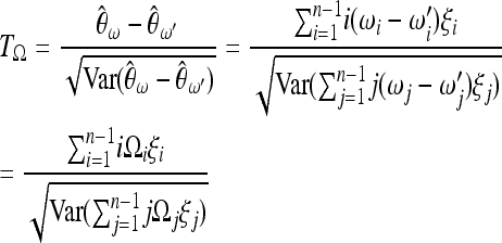
Given the common structure of the existing tests, it is actually possible to include these tests in a more general framework (Achaz 2009). In this framework it is possible to build a large number of new and promising tests generalizing Tajima's D test. In fact it is sufficient to choose any pair of unbiased estimators of θ based on the frequency spectrum

(2)

with weights , that obey the conditions = 1, = 1, to obtain a new test for neutrality,

(3)

(Achaz 2009), where is a set of weights satisfying the condition .

The number of tests that can be devised in this framework is virtually infinite. They include all the well-known tests of allele frequency proposed by Tajima (1989), Fu and Li (1993), Fu (1997), and Fay and Wu (2000), as well as the error corrections proposed in Achaz (2008) among other tests. Given the large number of possibilities, it would be useful to have some indications to decide which tests should be chosen for different analyses. Two basic and important questions arise naturally in this context:

• Which criteria should be followed while building new neutrality tests? Are there criteria to discriminate good choices of the weights , , and Ω_i from other (less good) ones?

• Is there an optimal way to choose the weights , , and Ω_i to obtain a test with maximum power? In other words, does an optimal test exist?

In this article we give a partial answer to both these questions.

About the first question, we note that a minimal requirement for a test is that its value on a sample from a population should not depend on the sample size, at least to a good approximation. This requirement translates into a condition on the scaling of the weights of the test with sample size. If this condition is not met, the interpretation of the result of the test is strongly dependent on the choice of the sample. A simple discussion of these points can be found in the next section.

For the second question, we argue that there cannot be an optimal test in terms of maximum power for a generic case (even if there could be tests that perform well in a wide range of situations). However, if there are some a priori expectations on the possible evolutionary or demographic scenario, a test can be built that maximizes its rejection power of the standard neutral model if the expected scenario is close to the actual one. Here, we propose a simple framework to derive optimal tests and we provide general formulas for the optimal scenario-dependent test. The main result of this article is a simple and explicit expression for the optimal test for genome-wide studies in terms of the expected spectrum , presented in Equation 9. Furthermore we present some examples of optimal tests based on simple scenarios, the possible generalizations and applications to the search for a generic optimal test. Tests and applications for the most common evolutionary scenarios will be implemented in the next version of DnaSP (Librado and Rozas 2009).

SAMPLE SIZE INDEPENDENT TESTS

As explained in the Introduction, the general form for the tests based on the spectrum ξ_i is shown in (3). In the framework presented by Achaz, a test is defined by a set of weights , with i = 1, 2, … , n − 1 only if the sample size n is fixed. An example is the test for bottleneck of Achaz (2009), which was proposed to detect a strong recent bottleneck in a sample of size n = 30. This test weights positively the low-frequency derived alleles and is defined by the weights

(4)

The optimal value of α reported in Achaz (2009) is ∼ .

In practice, this information is not sufficient to build a useful test. In fact, each set of data has a different sample size n and the definition of a test should include all reasonable values of n; that is, a test should be defined by a succession of sets of weights , . These weights should scale with n in such a way that the interpretation of the results of the test should be as independent on the sample size as possible. The good scaling of these weights with sample size n is an important issue when building neutrality tests on the basis of the above framework.

As an example of an unfortunate choice of scaling, consider the test for bottleneck described above. The form (4) for the weights can be taken without modification for all values of the sample size n: this is a legitimate choice of scaling and the weights are normalized correctly for all values of n. However, the total weight of the frequencies between f = 0.15 and 0.25 is Ω = 0.13 for n = 10, but it changes sign becoming Ω + … + Ω = − 0.1 for n = 100 and the has same value for n = 1000. This means that a spectrum with a strong excess of alleles in this range of frequencies appears as a large positive value of the test for a sample of size n = 10, but has a large negative value for n = 100 and 1000.

It is clear from this example that the interpretation of the results of this test depends critically on the sample size n. Since modern sequencing technologies allow one to deal with data from studies with different numbers of individuals, ranging from small projects of 5–10 individuals to the large-scale projects like 1000 Genomes for humans or 1001 Genomes for Arabidopsis, it would be advisable to have consistent tests whose results could be interpreted in a standard way without referring to the size of the sample. This is not always possible, but it should be taken into account when building new generalized neutrality tests.

There is a simple scaling that does not suffer from this problem. The recipe is to write the weights as functions of the frequency f = i/n instead of the allele count i. These weight functions ω(f), ω′(f) should not depend explicitly on n. Then these functions can be easily normalized to obtain the weights

(5)

For the example above, the dependences of ω and ω′ on i are exponential and uniform, respectively, and therefore the weight functions should have the form ω(f) ∝ e^−βf, ω′(f) ∝ 1 and the scaling of the weights becomes

(6)

The corresponding optimal value for β should be ∼ . With this scaling, the total weight of the frequencies between f = 0.15 and 0.25 is Ω = −0.05 for n = 10 and Ω + … + Ω = −0.08 for n = 100 and n = 1000. An excess of alleles in this range of frequencies would therefore give similar negative values for the test for these three sample sizes, making it possible to have an interpretation independent of sample size.

The recipe (5) is simple and gives a rule of thumb to build new neutrality tests in this framework. This rule is valid for all frequencies with the important exception of singletons. The reason is that singletons are quite sensitive to an excess or a lack of alleles not only at frequencies of order 1/n but also at lower frequencies. For this reason they can be assigned a different weight from the one suggested by the above discussion, particularly in tests that should take into account deviations from the null spectrum at very low frequencies. An important example is given by the tests of Fu and Li (1993).

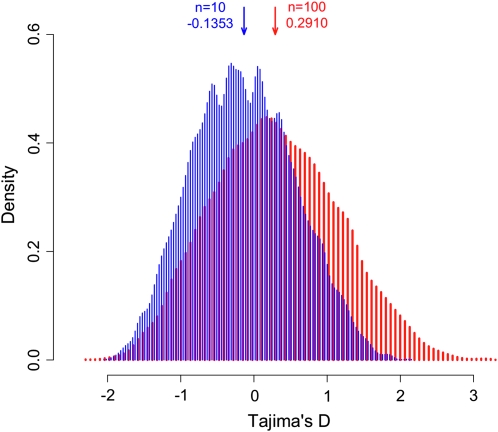
We end this section with a remark: there are some relevant tests for which the rule (5) cannot ensure independency of the value of the test from sample size. This is the case for most of the tests containing the Watterson estimator (Watterson 1975). As an example we focus on the important case of Tajima's D, which is based on the difference between pairwise nucleotide diversity (Tajima 1983) and the Watterson estimator. This test scales according to the rule (5) with weight functions ω(f) = 2(1 − f) and ω′(f) ∝ 1/f. If we consider a spectrum with a strong excess of alleles at frequencies ∼f = 0.2 in the population (for example, an admixture between a small and a large population), we see from Figure 1 that the distributions of the results of Tajima's D for n = 10 and n = 100 are different and moreover that the distribution for n = 10 has a negative average (E(D) = − 0.14) while the distribution for n = 100 has a positive average (E(D) = +0.29).

Figure 1.—

Frequency distribution of Tajima's D for n = 10 (blue) and n = 100 (red) for a frequency spectrum with an excess of alleles between 0.1 and 0.2. The distributions were obtained from simulations of an admixture of two populations (one single population split in two isolated at 0.2N_e generations from present, with N_e1 = 0.15N_e and N_e2 = 0.85N_e, and merged 8N_e generations later). A short period of high recombination values was used at the beginning (first 0.2N_e generations) to reduce the effect of discrete sampling from one or the other population, especially in the case of n = 10.

The problem in this example lies in the weights = 1/ia_n of the Watterson estimator. The reason is that for increasing values of n, these tests assign very high weights to very low frequencies that were practically not represented in samples of smaller size; therefore the normalization of the weights has a nonnegligible dependence on sample size and the relative value of the weights with respect to gets distorted. This issue cannot be addressed in any way; therefore some care is needed while interpreting the results of Tajima's D and similar tests based on the Watterson estimator. In other words, it is true that Tajima's D gives a positive value when the spectrum shows an excess of intermediate-frequency alleles and a negative value for an excess of low- and high-frequency alleles, but the definition of low frequency depends on sample size. Since this dependence is logarithmic, the effect is usually not strong.

OPTIMAL NEUTRALITY TESTS

While the above result on the scaling of generalized neutrality tests shows that a test could be encoded in functions like ω(f) and ω′(f), it tells nothing on the optimal form of these functions or on the optimal weights Ω . The problem of finding an optimal test is a difficult one, at least if the test should be optimal for all possible scenarios. This is a consequence of the linearity of these tests. In fact, for every test in this framework there are some allele frequencies that are positively weighted and some others that are negatively weighted, and then the linearity implies that it is always possible to find a spectrum such that the average of the test on this spectrum is zero and therefore the test is far from optimal for the corresponding scenario. However, if we have some expectation on the possible demographic or selective scenario that originated the pattern of the sample, we can optimize the test to reject the standard Wright–Fisher model in this specific scenario.

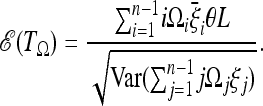
Assume that we expect that the data would follow a scenario where the expected spectrum is . The generalized test T_Ω applied to this spectrum gives an average value of

(7)

The criterion that we propose to find an optimal test is to choose the weights that maximize the expected value of the test, given the alternative spectrum. Since the variance of the test is equal to 1, this choice should approximately maximize the average rejection power.

Optimal neutrality tests for genome-wide data:

To simplify further the results, we assume independent sites and . This is equivalent to the composite-likelihood approach and is a good approximation for genome-wide studies. In this approximation the covariances Cov(ξ_i, ξ_j) are negligible and the variances are equal to the means E(ξ_i) = Var(ξ_i) = θL/i. The problem reduces to constrained maximization with the condition . Using the method of Lagrange multipliers (see the derivation in supporting information, File S1), the optimal weights are

(8)

that is, the difference of the expected frequencies and the frequencies under the neutral model. The optimal test is therefore

(9)

This result is remarkable in several aspects. It is a simple formula with a clear structure: the optimal test is always proportional to the difference between a scenario-dependent estimator of θ, whose weights are the expected frequencies , and the Watterson estimator.

The interpretation of the test is the following:

• Significant positive result: the data appear to reject the neutral model and to be consistent with the expected scenario.

• Result close to zero: the neutral spectrum cannot be rejected and there is no evidence for the expected scenario. The observed deviations from the null spectrum are small or they are different from the expected ones.

• Significant negative result: the data appear to reject the neutral model and to exclude the expected scenario, because the observed deviations from the null spectrum are opposite to the expected ones.

In fact, by writing the numerator of the above expression as

(10)

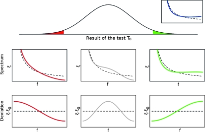
it is clear that the value of T_O is always positive (and almost maximum if the covariances are negligible) when the observed spectrum corresponds to the expected one, i.e., if , while it is negative (and almost minimum) if the observed spectrum shows deviations from the standard spectrum that are opposite to the expected ones, i.e., if there is an excess of alleles at frequencies where a lack of alleles is expected and vice versa. If the result of the test is close to 0, this means that the deviations of the observed spectrum from the usual spectrum show a pattern that is completely uncorrelated with the expected one. Figure 2 illustrates the different cases.

Figure 2.—

Possible results of an optimal test T_O. The test is built for the expected spectrum shown in blue at top right, where the dashed line represents the spectrum ξ₀ under the neutral model. The main plot shows a possible distribution of the results of the test T_O for the standard neutral model. The value of the tests can be significant and positive (in green) or negative (in red) or not significant. The plots below show examples of spectra ξ (as functions of the allele frequency f) leading to negative, not significant, or positive values of the test (the black dashed lines correspond to the neutral spectrum). The deviations of these spectra from the neutral model are shown in the plots at the bottom. Note that the red line corresponds to a frequency of rare derived variants larger than expected, opposite to what is assumed (the blue line).

The variance in the denominator of test (9) can be evaluated analytically in the approximation of infinite or zero recombination. We denote the corresponding tests as and , respectively. We report the formulas in File S1.

Optimal neutrality tests for data without recombination:

The above tests are obtained using approximations that are not correct for small regions in strong linkage disequilibrium, because in this case the θ² terms in the covariances Cov(ξ_i, ξ_j) represent the biggest contribution to the total variance. However, in this case it is still possible to pursue the above approach of maximizing . We define the matrix , where is an estimator of θ (for example, S/a_nL). The explicit expression for Cov(ξ_i, ξ_j) for the case without recombination can be found in Fu (1995) (Equations 1–5; note the different convention θ_(FU) = θ_(our)L). The optimal weights resulting from constrained maximization are

(11)

where is the i, jth element of the inverse matrix of the covariance matrix, that is, . This expression is cumbersome but it can be easily implemented numerically.

Since the covariance matrix c_ij and its inverse are real, symmetric, and positive, it is easy to show that the value of T_O is positive and maximum when the observed spectrum corresponds to , and therefore the interpretation of the results of the test does not change with respect to the previous case.

If the covariance matrix c_ij corresponds to the case of zero recombination, we denote the above test by . However, the above expression (11) is actually more general than the case of no recombination. In fact it is valid for all cases when the full covariance matrix has to be taken into account. However, in practice the covariance matrix is often unknown or there is no analytical expression for it. In these cases a quasi-optimal test could be implemented by using analytical approximations (if available) to the exact matrix.

Expressions similar to (9) and (11) can also be found for optimal tests based on the folded spectrum. It is also possible to include error corrections along the line of Achaz (2008). We report the corresponding formulas and proofs in File S1.

Optimal test for a general (complex demographic) null model spectrum:

A generalization that could prove useful for more refined studies is the application of the test to reject a general null model (i.e., typically a complex demographic model). An interesting case could be a test for selection on a sample from a population with nontrivial demographic dynamics, e.g., bottlenecks, expansion, or migration. In this case a first analysis would concentrate on the demographic dynamics, whose signatures could be found along the whole genome, and then this information could be used in a refined analysis to build a test against this null model and look at regions showing signatures of selection or other evolutionary processes.

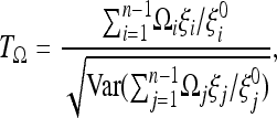
We assume that the general null model has a spectrum E(ξ_i) = ξ θL and the corresponding covariance matrix c_ij = E(ξ_iξ_j) − E(ξ_i)E(ξ_j). These data can come from theoretical results (like the second moments obtained by Zivkovic and Wiehe 2008 for a model with varying population size) or simulations of the null model, or they can be directly inferred from the empirical data, e.g., looking at noncoding regions or genome-wide patterns. For this null model, a set of unbiased estimators of θ based on the unfolded frequency spectrum is , which can be combined with weights ω_i to build unbiased estimators . A general test for neutrality can therefore be written as

(12)

where the variance in the denominator is evaluated under the general null model.

The simplest results can be obtained by employing the approximation of independent sites and . In this case the random variables ξ_i(s) for each site s are independent binomial variables with range {0, 1}; therefore the variables satisfy the relations Var(ξ_i) = E(ξ_i) = ξθL. From these relations we can derive the optimal tests

(13)

We denote this class of tests by T_OH0. Formulas for the other cases (generic covariance matrix and folded spectra) can be found in File S1.

APPLICATIONS

Tests for usual demographic and selective models:

Optimal tests are defined with respect to a given expected spectrum . In some cases, this spectrum could be obtained from coalescent simulations or experimental data. However, the best way to find it is to obtain an explicit formula for the spectrum from a simple analytical model for the expected scenario; the values will be functions of the parameters of the scenario itself. In this way, the spectrum depends fully on the choice of a simple scenario and of its parameters.

In this section, we present some explicit formulas for some simple and common scenarios of population genetics: positive selection, bottleneck, expansion, and contraction. These are only examples of the possible models that could be used to build new optimal tests and do not intend to be an exhaustive list of the best models that could be used for this purpose.

Before discussing the expected spectra, it is worth noting that the optimal test does not actually depend on the spectrum , but only on the deviations from the null distribution. Moreover, only the form of these deviations is relevant, while their overall magnitude is not (see Theorem 3 in File S1).

Note that, if the expected spectrum of the whole population is known, the weights of the test for a given sample size n can be obtained directly from binomial resampling from the spectrum :

(14)

This also shows that the weights follow the scaling (5) only for large sample size, while for small sample size they scale according to binomial sampling in a natural way.

Test for positive selection:

The article by Kim (2006) contains approximated expressions for the spectra of single and recurrent selective sweeps obtained through diffusion approximation. The spectrum for a single sweep depends on the recombination fraction r and the time τ since fixation in units of 4N generations. The spectrum can be calculated from Equation 2 of Kim (2006) and equations thereafter, by substituting the coefficients defined in the Appendix of the same article.

Test for bottleneck:

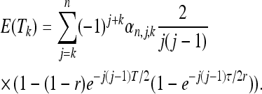
The spectrum for a neutral model with varying population size based on the coalescent approach is presented in Griffiths and Tavaré (1998) and Zivkovic and Wiehe (2008). We review the formulas using the same notation as the latter article. The allele spectrum after a bottleneck depends on three parameters: the time distance T from the bottleneck, the duration τ of the bottleneck, and the magnitude 1/r = N/N_min, that is, the ratio between the normal population size and its size during the bottleneck. Both T and τ are in units of 2N generations. The expression of the spectrum is given by Equations 1 and 10 of Zivkovic and Wiehe (2008) in terms of waiting times E(T_k) dependent on the scenario. For a bottleneck of strength r = N_min/N that ended T generations ago and lasted for τ generations, their expression is

(15)

Test for sudden expansion/contraction:

This scenario depends on two parameters: the time distance T from the expansion/contraction and the expansion/contraction parameter ρ. The spectrum for this case can be obtained following the same approach as the previous one (Equation 15). As in the previous example, the spectrum is a function of the waiting times E(T_k),

(16)

where T is the time (in units of 2N generations) from the change in population size and ρ is the ratio between the population size after and before the change. The case ρ > 1 corresponds to an expansion, while the case ρ < 1 corresponds to a contraction.

Testing a generic evolutionary scenario:

A possible problem of optimal tests is that they assume not only some knowledge of possible evolutionary or demographic scenarios, but also a good guess of their parameters. This can be quite difficult and subjective. For this reason, it would be interesting to develop more generic estimators. To discuss this issue, we can assume that the weights are calculated from a model of a given scenario that depends on a parameter ν. We denote by P₀(ν) a prior probability distribution for this parameter. The expected values for the ξ_i are

(17)

and the maximization of yields the optimal weights

(18)

This result is the straightforward extension of the approach presented in this article. Note that, from a practical point of view, all the integrals over ν in the above expressions can be substituted by sums over a discrete set of values to obtain a good numerical approximation to the test.

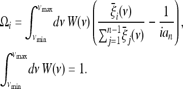
In practice the above approach is not always convenient because the number of segregating sites may vary with the parameter ν and, therefore, the spectra with a larger number of segregating sites will dominate the test. If we denote by ν_min and ν_max the extreme values for the typical range of values of the parameter ν, an alternative solution to obtain a generic test for this scenario would be a weighted form like

(19)

We denote these tests as T_OG. The function W(ν) can be chosen in different ways. If there is more than one order of magnitude between ν_min and ν_max, a good choice could be a lognormal distribution centered in or a distribution 1/ν (that is a constant distribution in logarithmic scale). Note that it is easier and computationally faster to take a discrete average over a set of values {ν₁, ν₂, … , ν_r} of the parameter

(20)

For models dependent on more parameters, either continuous or discrete, the above formulas can be generalized in a straightforward way by choosing P₀ or W as functions of the whole set of parameters and substituting the integral over ν with integrals over all the continuous parameters and sums over all the discrete ones. The same approach can be applied to the other cases detailed in this article.

Simulations:

The optimal tests proposed in this article are built using an analytical approach that should generally provide a relatively high power for the rejection of the standard neutral model. However, these tests are based on an optimality condition that does not take into account either the variance of the tests under the alternative model or the estimation of the parameter θ from the same data tested. Because of these issues, the actual power could be quite different from the maximum one. To understand the impact of these issues on the power of the tests, a computational study is unavoidable.

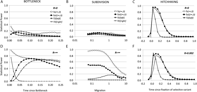
To check the actual power of optimal tests, we simulate a coalescent model with mlcoalsim v1.98b (Ramos-Onsins and Mitchell-Olds 2007), available from authors under different scenarios and parameters. The scenarios include bottleneck, migration, and selection (see Figures 3 and 4). We obtain the optimal tests both for the specific choices of parameters and for the generic scenario, inferring the expected spectrum from the simulations. Finally we apply several tests to simulated data, including optimal tests (both specific and generic) and Tajima's D, comparing their power to detect deviations from the standard neutral model.

Figure 3.—

Statistical power of T_O tests and Tajima's D test for a sample n = 20 and θ = 0.05 per nucleotide in a region of 1000 nucleotides for a given alternative model (expansion, subdivision, or hitchhiking) and for different values of recombination R = 4N_er. The null (stationary) model and the alternative model were compared using the same recombination rate. Open circles represent T_O^(∞,0) left tail, solid circles represent T_OG^(∞,0) left tail, stars represent Tajima's D left tail, and +'s represent Tajima's D right tail. Type I error was set to 0.025 for each tail. (A and D) Bottleneck model: the x-axis shows the time (measured in 4N_e generations) since a stationary population suddenly dropped 0.1 × N_e times and recovered 0.05 × 4N_e generations later (from present to past); recombination R = 0 (A) and R = ∞ (D). T_OG is based on a uniform distribution over a range of time since bottleneck between 0.001 and 0.25 × 4N_e generations. (B and E) Subdivision model: the x-axis shows different values of migration (M = 4N_em) between two populations of equal size. T_OG is based on a log-uniform distribution over a range of migration values (4N_em) between 0.05 and 10; recombination R = 0 (B) and R = ∞ (E). (C and F) Hitchhiking model: a region located 40 kb left of the studied region experienced a selective event with a fitness value s = 2 × 10⁴ in a population of N_e = 1 × 10⁶. The x-axis shows the time since the selective variant was fixed in the population, ranging from −0.1 (still not fixed) to 1.0 in 4N_e generations. The same range was used for T_OG with uniform distribution. Recombination R = 0 (C) and R = 0.002 per nucleotide (F).

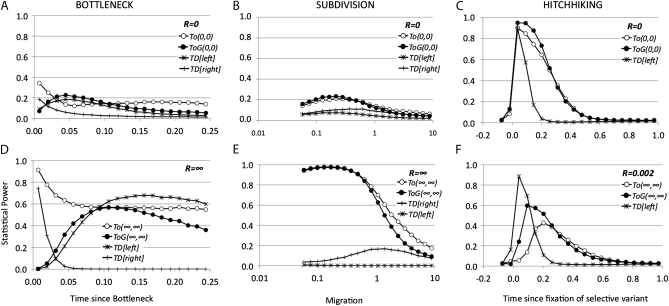
Figure 4.—

The same as Figure 3 except that for A–C the open circles represent the statistical power for the left tail of T_O^(0,0) and solid circles represent T_OG^(0,0), and for D–F the open circles represent T_O^(∞,∞) and solid circles represent T_OG^(∞,∞).

All the tests employed are based on the unfolded spectra. We implement the test for the case of no recombination on the basis of Equation 11, the test on the basis of (9) for the case of infinite recombination, and finally the test also on the basis of (9), which should have maximum power for infinite recombination but whose variance is calculated for the case of no recombination. Tajima's D, Fay and Wu's H normalized, and other tests belong to the last class of tests. We implement also generic versions T_OG of all these tests for the generic scenarios, on the basis of Equation 19 and generalizations.

As is clear from Figures 3 and 4, optimal tests are actually far more powerful than Tajima's D in most situations. In some cases, the generic optimal test (T_OG) can be more powerful than the specific one. The cause of these phenomena may be the difference in the variance associated with the tests: a generic test should be suboptimal but it could have higher power than the optimal test for a specific condition, if the variance of the latter is larger. In most cases the T_O and the T_OG tests have similar power. A clear exception is observed in the subdivision model for T_O^(∞,0) and T_OG^(∞,0) tests and R = ∞, where T_OG^(∞,0) is very low and even drops at the level of Tajima's D at some parameters. In some specific scenarios, Tajima's D is superior to the optimal test T_O^(∞,∞) (Figure 4, D and F). In the second case this test is compared with optimal tests of the type T_O^{(∞, ∞)} but using a rescaled recombination rate of R = 0.002 per nucleotide that is much smaller than the rescaled mutation rate. In the same case, the power of the optimal tests T_O^{(∞, 0)} or T_O^{(0, 0)} is higher than Tajima's D. Finally, for the case of the bottleneck, note that the frequency spectrum changes significantly from bottleneck times before or after 0.03 × 4N_e generations, as indicated by the change in statistical power for the right and the left tails in Tajima's D. Therefore, a general test for the whole set of parameters could be not powerful enough in at least one of the specific scenarios. Here, the test T_OG has no power for the scenarios resembling a contraction scenario (from 0.1 to 0.03 × 4N_e generations).

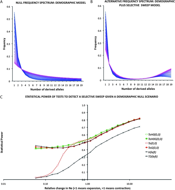
Figure 5 shows the frequency spectrum for several scenarios and the power of the optimal test with a generic null spectrum (12), indicated here as T_OH0^{(0, 0)}. As a null model we choose sudden contraction/expansion with the ratio of ancient vs. present population size ranging from 0.05 (expansion) to 20 (contraction), while in the alternative scenarios we add a selective sweep on the top of the corresponding null model. Figure 5, A and B, shows the spectra of null and alternative models, respectively. Clearly, unless extreme situations occur ( ), all tests proposed are more powerful than standard Tajima's D and almost all of them are as powerful as Fay and Wu's H (Figure 5C). The optimal test with generic null spectrum T_OH0^{(0, 0)} is more powerful than the optimal test T_O^(0,0) only for expansion, where the power of T_O^{(0, 0)} drops down.

Figure 5.—

Simulation results for the analysis of a null demographic model vs. the same demographic model but where a selective sweep occurred. (A) Frequency spectrum for the null demographic model. The colors from blue to pink indicate the frequency spectrum for 20 conditions tested, going from strong expansion models (dark blue, N₀/N = 0.05) to strong contraction (pink, N₀/N = 20). A log-uniform distribution was used for T_OG. (B) Frequency spectrum for the null demographic model plus selective sweep. The colors from blue to pink indicate the frequency spectrum for different demographic conditions tested, as explained in A. (C) Statistical power of the optimal tests T_OH0^(0,0), T_O^(0,0) and the generalized tests for the entire studied parameters T_OG_H0^(0,0) and T_OG^(0,0) as well as Tajima's D and Fay and Wu's H normalized. The x-axis indicates the value of the relative change in N_e, from 0.05 (20× expansion) to 20 (20× contraction) in a log scale. A total of 5 × 10⁴ iterations/condition for H0 and for H1 were used to calculate the power. Coalescent simulations were run with n = 20, length = 1 kb, θ = 0.01 per nucleotide, time to change N_e = 0.1 × 4N_e, initial N_e = 10⁶, 4N_es = 2000, and selective event occurred at time 0 (present) at 20 kb from the studied region. Recombination R = 0.01 per nucleotide.

Analysis of sequence data from European pig breeds:

In this section we provide an example of an application of optimal tests on real sequence data (Ojeda et al. 2006). Moreover, we outline a useful application of the optimal tests for exploratory analysis that takes advantage of the connection between an optimal test and the corresponding spectrum under the alternative scenario.

The idea is that, for a given data set, the maximum (average) value for a test of the form (3) on these data is the value of the optimal test corresponding to the spectrum of the data. This is an immediate consequence of our definition of optimality. Moreover, the value of an optimal test is a continuous function of the expected spectrum. These observations imply that, in a set of optimal tests corresponding to different scenarios and parameters, the test with the highest value will correspond to the expected spectrum that is the “closest” to the actual spectrum of the data.

To implement this idea, we choose a generic scenario, we vary the values of its parameters, and we calculate the corresponding optimal tests. Then we look for the maximum value among the results of the tests and obtain the parameters corresponding to this maximum. These parameters should be close to the most probable parameters for this scenario.

We analyze a set of data from Ojeda et al. (2006) that consists of 8-kb sequences from the gene FABP4 in chromosome 4. For this study, we selected the sequences from European breeds (41 sequences) and the bases without gaps or missing values (3.5 kb). The demographic history of European and Asian pig breeds is complicated, but here we assume a simplified model (Larson et al. 2007). In this model the European population derives from an ancestor whose population originated also other Asian breeds. The European and Asian populations remained essentially separated until recent centuries, when Asian animals were crossed with European animals with a resulting introgression of Asian alleles in the European breeds. This introgression was actually followed by a process of artificial selection that we ignore in this analysis.

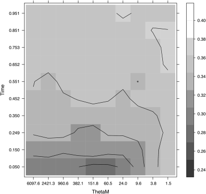
We obtain the spectrum of this simplified model from coalescent simulations, implementing the introgression of Asian alleles in the population as a migration process from another population with no fixed differences but a very high nucleotide variability. This model is actually equivalent to a strong sudden expansion, as shown in File S1. The scenario has two parameters, the time T_M since the migration started and the product θ_M = MH_A of the rescaled migration rate M and the heterozygosity H_A in the Asian population. The set of data is too small and does not allow us to reject the standard neutral model (at least without using haplotype information); consequently, the values of the optimal tests are small and cannot be compared because of the differences in the distributions of the tests, but we can use their P-values instead. Figure 6 shows the different P-values of the test T_O^{(0, 0)} as a function of the parameters T_M, θ_M. We observe the lowest P-values for small values of T_M and between 60 and 150 units for θ_M. Assuming a variability H_A = 0.001, these numbers correspond to M ∼ 30, i.e., a very high migration rate having occurred very recently. These results concord with historical evidence whereby Chinese pigs were imported into Europe repeatedly after the 17th century (Giuffra et al. 2000) and, importantly, also with the Bayesian inference using data from this same chromosome region in a wide panel of European and Chinese pigs (Ojeda et al. 2010).

Figure 6.—

Plot showing the P-value of the test T_O^0,0 for a grid of two parameter values (T_M, the time since the migration started in the y-axis, and θ_M = MH_A, the rescaled migration rate M and the heterozygosity H_A in the Asian population in the x-axis). The different shadings indicate the P-value of the optimal test for the parameter values indicated. The lower the P-value, the darker is the shading in the grid.

Note that from a strict statistical point of view, this approach should be taken with care if the aim of the analysis is simply the rejection of the null hypothesis, because there are issues related to multiple testing. These issues are not as severe as they appear, because most of the tests corresponding to different values of the parameters for a given scenario are actually related, but they should not be overlooked.

If there are no plausible expected scenarios for the data, it is also possible to infer the generic scenario that looks more similar to the data. It is sufficient to repeat the above procedure not for different values of the parameters of a single generic scenario, but for different generic scenarios, and infer the most plausible one simply by comparing the values of the corresponding optimal tests. Note that this approach works only with generic scenarios and not with specific scenarios dependent on some parameters, because otherwise the different number of parameters for each scenario should be taken into account and scenarios with more parameters should be penalized. These issues certainly merit further studies.

DISCUSSION

Although there is a wide literature on the power of Tajima's D (Tajima 1989), Fu and Li's F (Fu and Li 1993), and Fay and Wu's H (Fay and Wu 2000) under different demographic and selective scenarios (e.g., Braverman et al. 1995; Simonsen et al. 1995; Fu 1997; Ramos-Onsins and Rozas 2002; Depaulis et al. 2003; Ramos-Onsins et al. 2007; Ramírez-Soriano et al. 2008), there are not many works proposing new tests of this kind (Fu 1997; Zeng et al. 2006; Achaz 2008). Moreover, Tajima's D, Fu and Li's F, and Fay and Wu's H were built on qualitative reasoning about the different weights of low, intermediate, and high frequencies for different estimators of θ. The recent work by Achaz (2009) was the first systematic study of this general class of tests. In the general framework presented there, an infinite number of new tests based on the frequency spectrum could be built. However, this framework needs to be complemented by rules on the scaling of these tests with the sample size, as explained in the first section of results. Furthermore the way to find the better or the most powerful tests in this framework remained an open and relevant issue.

In this work we present a general answer to this question. In particular, we presented an explicit form for the optimal tests, i.e., the tests that have approximately maximum power to reject the standard neutral model if the data follow the chosen scenario. Some approximations for genome-wide data are also discussed, along with some useful generalizations like the optimal tests with general null spectrum. The key result is contained in the approximated expression (9). This expression is a generalization of Tajima's D optimized for an alternative spectrum . Similar expressions have been found for the folded spectrum, for the case of linked sites in Equation 11 and for a general null model in Equation 12. If the spectrum of the data is similar to , the above tests are more powerful than Tajima's D or any other tests of this kind.

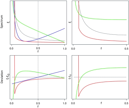
We note that optimal tests are actually a direct generalization of Tajima's D, Fu and Li's F, and Fay and Wu's H. In fact all these tests are instances of optimal tests (up to small corrections of order 1/n); that is, each of them has (almost) maximum power for a particular alternative spectrum. These spectra are not uniquely defined. We report them in File S1, Table 1. As illustrated in Figure 7, these alternative spectra show features that agree with the common understanding of these tests: Tajima's D is optimal against a spectrum with an excess of intermediate alleles and a defect of low-frequency alleles, while Fu and Li's F is sensitive to very rare alleles and Fay and Wu's H is optimal against an excess of high-frequency alleles and a defect of low-frequency alleles.

Figure 7.—

The plots at the top illustrate the spectra ξ for which different classical tests have maximum power: Tajima's D (green), Fu and Li's F (red), and Fay and Wu's H (blue). The black dashed lines correspond to the neutral spectrum. The unfolded spectra are on the left (the vertical dotted line corresponds to frequency f = 0.5) and the folded spectra are on the right. (Fay and Wu's H test works only with unfolded data.) In the bottom plots, the deviations from the null spectrum ξ₀ are shown. The plots are obtained for N_e = 1000 and .

Before discussing the possible applications of these tests, we comment on some issues related to the optimality condition proposed here. The condition of optimality that we propose is the maximization of , that is, the average value of the test when evaluated on the expected spectrum or . The advantage is that both the condition and the form and interpretation of the resulting tests are very simple. However, this condition corresponds to maximization of the power to reject the neutral Wright–Fisher model only if the distribution of the possible values of the test p(T_Ω = t) under this model is well approximated by a Gaussian for all choices of weights and if the covariance matrix of the alternative spectrum is proportional to the covariance matrix of the null spectrum. In the remaining cases, it is possible to find tests with higher power by imposing directly the condition of maximum power. We do not pursue this road because tests with maximum power have three important disadvantages: first, these tests depend explicitly and in a strong way on the significance value chosen, and therefore the results of the tests between different experiments are not comparable; second, they are cumbersome to derive, to implement, and to interpret; and third, they require the knowledge of second- (and higher)-order moments of the spectrum ξ_i under both the null and the expected scenario. This information is usually unavailable since third and higher moments are not known even for the neutral Wright–Fisher model without recombination and there is no analytic expression even for the second moments in the realistic case of finite recombination. This approach should be compared with the simple and clear optimality condition proposed in this article, which uses only information on the first moments of the alternative spectrum, and the simple form of the tests resulting from this condition.

The optimal tests discussed in this article can be useful as summary statistics, in particular for genome-wide data, and to get hints of demographic or selective processes. These tests can be simply used as more powerful versions of existing tests like Tajima's D, Fu and Li's F, or Fay and Wu's H, once some information about the expected scenario is known. However, there could be more efficient ways to employ these tests using the connection between them and the expected spectra. In particular there are two interesting applications of optimal tests that, in our opinion, deserve future work, which is mentioned at the end of the applications section.

The first one is the development of more generic tests. The optimality condition proposed in this article is not generic, but depends on the prior knowledge of the possible deviations from the standard spectrum. A generic test that does not use prior assumptions about the spectrum could be more useful and of wider applicability. However, it is likely that a completely generic test does not exist because there are deviations from the standard neutral model for every conceivable test that cannot be detected efficiently. Formal arguments for this claim are given in File S1. As discussed in results, there are tests like (18) and (19) that should be effective in a wider range of scenarios than the tests based on Equation 9. Actually, there can be different ways to build more generic tests using the above results, but their optimization is beyond the scope of this article.

The second one is the inference of population genetics models and parameters, which is a completely different way to implement optimal tests without requiring prior knowledge of the possible scenarios and their parameters. In fact, since these tests are computationally fast, it is possible to calculate the values of many different tests on a given set of data. In this way, these tests could scan a good fraction of the interesting parameter space for a specific scenario and give some hints on the relevant parameters. A simple example of this approach is presented in the context of data analysis of pig sequences in the last section of applications. This approach is particularly easy to automatize and can be used for exploratory analysis: by implementing it for some of the most common scenarios, like the ones presented in results, it is possible to infer automatically the most plausible scenario and its parameters by looking at the highest values of the tests. We emphasize that this approach should be applied in this form only for exploratory analysis and not for proper statistical inference. The study of a more rigorous statistical approach to infer scenarios and parameters from optimal tests, applying the ideas presented above, would be a most useful development. For example, it would be worth studying the use of these optimal tests (or the related estimators of θ) as summary statistics for statistical inference of evolutionary scenarios, possibly using approximate Bayesian computation, similarly to what is suggested in Achaz (2009). An interesting possibility could be to substitute the distance between summary statistics in approximate Bayesian computation analysis with a function of the P-values of optimal tests.

References

- Achaz, G., 2008. Testing for neutrality in samples with sequencing errors. Genetics 179 1409. [DOI] [PMC free article] [PubMed] [Google Scholar]
- Achaz, G., 2009. Frequency spectrum neutrality tests: one for all and all for one. Genetics 183 249. [DOI] [PMC free article] [PubMed] [Google Scholar]
- Braverman, J. M., R. R. Hudson, N. L. Kaplan, C. H. Langley and W. Stephan, 1995. The hitchhiking effect on the site frequency spectrum of DNA polymorphisms. Genetics 140 783–796. [DOI] [PMC free article] [PubMed] [Google Scholar]
- Depaulis, F., S. Mousset and M. Veuille, 2003. Power of neutrality tests to detect bottlenecks and hitchhiking. J. Mol. Evol. 57(Suppl. 1): S190–S200. [DOI] [PubMed] [Google Scholar]
- Fay, J., and C.-I. Wu, 2000. Hitchhiking under positive Darwinian selection. Genetics 155 1405. [DOI] [PMC free article] [PubMed] [Google Scholar]
- Fu, Y., and W.-H. Li, 1993. Statistical tests of neutrality of mutations. Genetics 133 693. [DOI] [PMC free article] [PubMed] [Google Scholar]
- Fu, Y.-X., 1995. Statistical properties of segregating sites. Theor. Popul. Biol. 48 172–197. [DOI] [PubMed] [Google Scholar]
- Fu, Y.-X., 1997. Statistical tests of neutrality of mutations against population growth, hitchhiking and background selection. Genetics 147 915. [DOI] [PMC free article] [PubMed] [Google Scholar]
- Galtier, N., F. Depaulis and N. Barton, 2000. Detecting bottlenecks and selective sweeps from DNA sequence polymorphism. Genetics 155 981. [DOI] [PMC free article] [PubMed] [Google Scholar]
- Giuffra, E., J. Kijas, V. Amarger, O. Carlborg, J. Jeon et al., 2000. The origin of the domestic pig: independent domestication and subsequent introgression. Genetics 154 1785. [DOI] [PMC free article] [PubMed] [Google Scholar]
- Griffiths, R., and S. Tavaré, 1998. The age of a mutation in a general coalescent tree. Stoch. Models 14 273–295. [Google Scholar]
- Hudson, R., M. Kreitman and M. Aguadé, 1987. A test of neutral molecular evolution based on nucleotide data. Genetics 116 153. [DOI] [PMC free article] [PubMed] [Google Scholar]
- Kim, Y., 2006. Allele frequency distribution under recurrent selective sweeps. Genetics 172 1967. [DOI] [PMC free article] [PubMed] [Google Scholar]
- Larson, G., U. Albarella, K. Dobney, P. Rowley-Conwy, J. Schibler et al., 2007. Ancient DNA, pig domestication, and the spread of the Neolithic into Europe. Proc. Natl. Acad. Sci. USA 104 15276–15281. [DOI] [PMC free article] [PubMed] [Google Scholar]
- Lewontin, R., and J. Krakauer, 1973. Distribution of gene frequency as a test of the theory of the selective neutrality of polymorphisms. Genetics 74 175. [DOI] [PMC free article] [PubMed] [Google Scholar]
- Librado, P., and J. Rozas, 2009. DnaSP v5: a software for comprehensive analysis of DNA polymorphism data. Bioinformatics 25 1451. [DOI] [PubMed] [Google Scholar]
- Nielsen, R., 2005. Molecular signatures of natural selection. Annu. Rev. Genet. 39 197–218. [DOI] [PubMed] [Google Scholar]
- Ojeda, A., J. Rozas, J. M. Folch and M. Perez-Enciso, 2006. Unexpected high polymorphism at the FABP4 gene unveils a complex history for pig populations. Genetics 174 2119–2127. [DOI] [PMC free article] [PubMed] [Google Scholar]
- Ojeda, A., S. E. Ramos-Onsins, D. Marletta, L. Huang, J. Folch et al., 2010. Evolutionary study of a potential selection target region in the pig. Heredity(in press). [DOI] [PMC free article] [PubMed]
- Ramírez-Soriano, A., S. E. Ramos-Onsins, J. Rozas, F. Calafell and A. Navarro, 2008. Statistical power analysis of neutrality tests under demographic expansions, contractions and bottlenecks with recombination. Genetics 179 555–567. [DOI] [PMC free article] [PubMed] [Google Scholar]
- Ramos-Onsins, S. E., and T. Mitchell-Olds, 2007. Mlcoalsim: multilocus coalescent simulations. Evol. Bioinform. Online 3 41–44. [PMC free article] [PubMed] [Google Scholar]
- Ramos-Onsins, S. E., and J. Rozas, 2002. Statistical properties of new neutrality tests against population growth. Mol. Biol. Evol. 19 2092–2100. [DOI] [PubMed] [Google Scholar]
- Ramos-Onsins, S. E., S. Mousset, T. Mitchell-Olds and W. Stephan, 2007. Population genetic inference using a fixed number of segregating sites: a reassessment. Genet. Res. 89 231–244. [DOI] [PubMed] [Google Scholar]
- Sabeti, P., D. Reich, J. Higgins, H. Levine, D. Richter et al., 2002. Detecting recent positive selection in the human genome from haplotype structure. Nature 419 832–837. [DOI] [PubMed] [Google Scholar]
- Sabeti, P., S. Schaffner, B. Fry, J. Lohmueller, P. Varilly et al., 2006. Positive natural selection in the human lineage. Science 312 1614. [DOI] [PubMed] [Google Scholar]
- Simonsen, K. L., G. A. Churchill and C. F. Aquadro, 1995. Properties of statistical tests of neutrality for DNA polymorphism data. Genetics 141 413–429. [DOI] [PMC free article] [PubMed] [Google Scholar]
- Tajima, F., 1983. Evolutionary relationship of DNA sequences in finite populations. Genetics 105 437. [DOI] [PMC free article] [PubMed] [Google Scholar]
- Tajima, F., 1989. Statistical method for testing the neutral mutation hypothesis by DNA polymorphism. Genetics 123 585. [DOI] [PMC free article] [PubMed] [Google Scholar]
- Wall, J., P. Andolfatto and M. Przeworski, 2002. Testing models of selection and demography in Drosophila simulans. Genetics 162 203. [DOI] [PMC free article] [PubMed] [Google Scholar]
- Watterson, G., 1975. On the number of segregating sites in genetical models without recombination. Theor. Popul. Biol. 7 256. [DOI] [PubMed] [Google Scholar]
- Zeng, K., Y.-X. Fu, S. Shi and C.-I. Wu, 2006. Statistical tests for detecting positive selection by utilizing high-frequency variants. Genetics 174 1431–1439. [DOI] [PMC free article] [PubMed] [Google Scholar]
- Zivkovic, D., and T. Wiehe, 2008. Second-order moments of segregating sites under variable population size. Genetics 180 341. [DOI] [PMC free article] [PubMed] [Google Scholar]