The Total Branch Length of Sample Genealogies in Populations of Variable Size

Abstract

We consider neutral evolution of a large population subject to changes in its population size. For a population with a time-variable carrying capacity we study the distribution of the total branch lengths of its sample genealogies. Within the coalescent approximation we have obtained a general expression—Equation 20—for the moments of this distribution with a given arbitrary dependence of the population size on time. We investigate how the frequency of population-size variations alters the total branch length.

MODELS for gene genealogies of biological populations often assume a constant, time-independent population size N. This is the case for the Wright–Fisher model (Fisher 1930; Wright 1931), for the Moran model (Moran 1958), and for their representation in terms of the coalescent (Kingman 1982). In real biological populations, by contrast, the population size changes over time. Such fluctuations may be due to catastrophic events (bottlenecks) and subsequent population expansions or just reflect the randomness in the factors determining the population dynamics. Many authors have argued that genetic variation in a population subject to size fluctuations may nevertheless be described by the Wright–Fisher model, if one replaces the constant population size in this model by an effective population size of the form

(1)

where N_l stands for the population size in generation l. The harmonic average in Equation 1 is argued to capture the significant effect of catastrophic events on patterns of genetic variation in a population: if, for example, a population went through a recent bottleneck, a large fraction of individuals in a given sample would originate from few parents. This in turn would lead to significantly reduced genetic variation, parameterized by a small value of N_eff. (See, e.g., Ewens 1982 for a review of different measures of the effective population size and Sjödin et al. 2005 and Wakeley and Sargsyan 2009 for recent developments of this concept.)

The concept of an effective population size has been frequently used in the literature, implicitly assuming that the distribution of neutral mutations in a large population of fluctuating size is identical to the distribution in a Wright–Fisher model with the corresponding constant effective population size given by Equation 1. However, recently it was shown that this is true only under certain circumstances (Kaj and Krone 2003; Nordborg and Krone 2003; Jagers and Sagitov 2004). It is argued by Sjödin et al. (2005) that the concept of an effective population size is appropriate when the timescale of fluctuations of N_l is either much smaller or much larger than the typical time between coalescent events in the sample genealogy. In these limits it can be proved that the distribution of the sample genealogies is exactly given by that of the coalescent with a constant, effective population size.

More importantly, it follows from these results that, in populations with variable size, the coalescent with a constant effective population size is not always a valid approximation for the sample genealogies. Deviations between the predictions of the standard coalescent model and empirical data are frequently observed, and there are a number of different statistical tests quantifying the corresponding discrepancies (see, for example, Tajima 1989, Fu and Li 1993, and Zeng et al. 2006). The analysis of such deviations is of crucial importance in understanding, for example, human genetic history (Garrigan and Hammer 2006). But while there is a substantial amount of work numerically quantifying deviations, often in terms of a single number, little is known about their qualitative origins and their effect upon summary statistics in the population in question.

The question is thus to understand the effect of population-size fluctuations on the patterns of genetic variation, in particular for the case where the scale of the population-size fluctuations is comparable to the time between coalescent events in the ancestral tree. As is well known, many empirical measures of genetic variation can be computed from the total branch length of the sample genealogy (the expected number of single-nucleotide polymorphisms, for example, is proportional to the average total branch length).

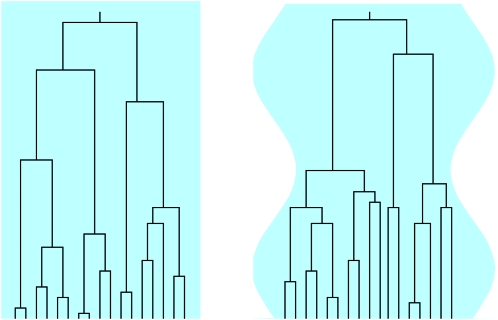
The aim of this article is to analyze the distribution of the scaled total branch length T_n for a sample genealogy in a population of fluctuating size, as illustrated in Figure 1. For the genealogy of n ≥ 2 lineages sampled at the present time, the expression ⌊NT_n⌋ gives the total branch length in terms of generations. Here ⌊Nt⌋ is the largest integer ≤Nt, and the scaling factor N is a suitable measure of the number of genes in the population and serves as a counterpart of the constant generation size of the standard Wright–Fisher model.

Figure 1.—

The effect of population-size oscillations on the genealogy of a sample of size n = 17 (schematic). Left, genealogy described by Kingman's coalescent for a large population of constant size, illustrated by the light blue rectangle; right, sinusoidally varying population size. Coalescence is accelerated in regions of small population sizes and vice versa. This significantly alters the tree and gives rise to changes in the distribution of the number of mutations and of the population homozygosity.

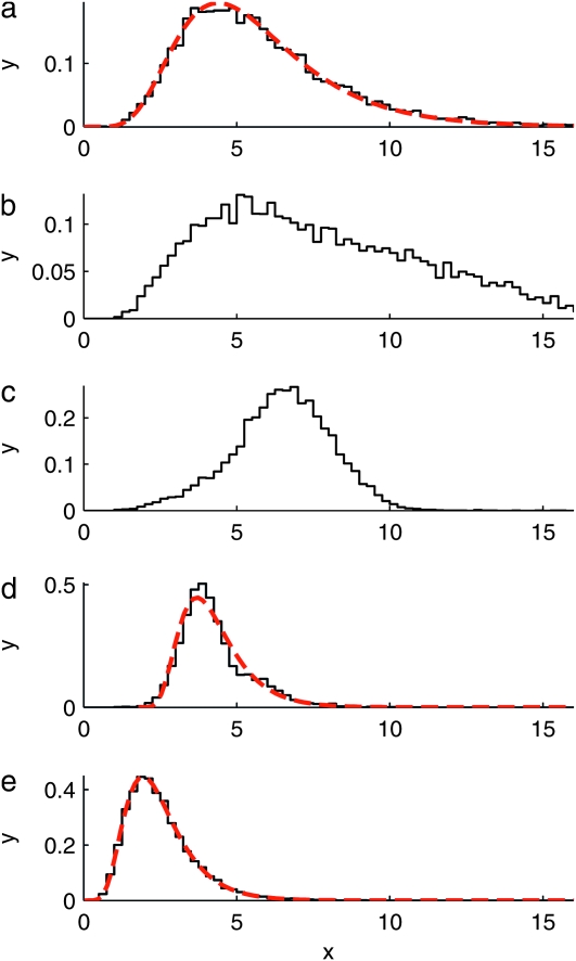
A motivating example is given in Figure 2, which shows numerically computed distributions ρ(T_n) of the total branch lengths T_n for a particular population model with a time-dependent carrying capacity. The model is described briefly in the Figure 2 legend and in detail in a model for a population with time-dependent carrying capacity. As Figure 2 shows, the distributions depend in a complex manner on the form of the size changes. We observe that when the frequency of the population-size fluctuations is very small (Figure 2a), the distribution is well described by the standard coalescent result

(2)

(Hein et al. 2005). When the frequency is very large (Figure 2e), Equation 2 also applies, but with a different time scaling reflecting an effective population size: t on the right-hand side (rhs) in Equation 2 is replaced by t/c with c = N/N_eff. Apart from these special limits, however, the form of the distributions appears to depend in a complicated manner upon the frequency of the population-size variation. The observed behavior is caused by the fact that coalescence proceeds faster for smaller population sizes and more slowly for larger population sizes, as illustrated in Figure 1. But the question is how to quantitatively account for the changes shown in Figure 2.

Figure 2.—

Numerically computed distributions of the scaled total branch lengths T_n in genealogies of samples of size n = 10. The model employed in the simulations is outlined in a model for a population with time-dependent carrying capacity. It describes a population subject to a time-varying carrying capacity, K_l = K₀(1 + ɛ sin(2πνl)). The frequency of the time changes is determined by ν, and l = 1, 2, 3, … labels discrete generations forward in time. The parameter N = K₀ describes the typical population size, which is taken here to be equal to the time-averaged carrying capacity. a–e show for populations with increasingly rapidly oscillating carrying capacity. The dashed red line in a shows that in the limit of low frequencies the standard coalescent result, Equation 2, is obtained. The dashed red line in e shows that also in the limit of large frequencies the standard coalescent result is obtained, but now with an effective population size. The dashed red line in d is a two-parameter distribution, Equation 41, derived in comparison between numerical simulations and coalescent predictions. Further numerical and analytical results on the frequency dependence of the moments of these distributions are shown in Figure 4. Parameter values used: K₀ = 10,000, ɛ = 0.9, and r = 1 (see a model for a population with time-dependent carrying capacity for the exact meaning of the intrinsic growth rate r) and (a) νN = 0.001, (b) νN = 0.1, (c) νN = 0.316, (d) νN = 1, and (e) νN = 100.

We show in this article that the results of the simulations displayed in Figure 2 are explained by a general expression—Equation 20—for the moments of the distributions shown in Figure 2. Our general result is obtained within the coalescent approximation valid in the limit of large population size. But we find that in most cases, the coalescent approximation works very well down to small population sizes (a few hundred individuals). Our result enables us to understand and quantitatively describe how the distributions shown in Figure 2 depend upon the frequency of the population-size oscillations. It makes possible to determine, for example, how the variance, skewness, and the kurtosis of these distributions depend upon the frequency of demographic fluctuations. This in turn allows us to compute the population homozygosity and to characterize genetic variation in populations with size fluctuations.

The remainder of this article is organized as follows. The next section summarizes our analytical results for the moments of the total branch length. Following that, we describe the model employed in the computer simulations. Then, corresponding numerical results are compared to the analytical predictions. And finally, we summarize how population-size fluctuations influence the distribution of total branch lengths and conclude with an outlook.

COALESCENT APPROXIMATION FORMULAS FOR THE MOMENTS

For the purpose of coalescent approximation it is convenient to introduce a “scaled time” t and a “scaled population size” x(t) by writing

(3)

Here N is a suitable counterpart of the constant generation size of the standard Wright–Fisher model assumed to be large. The population is sampled in generation l_s corresponding to t = 0, and the time t is now counted backward in units of N generations, as is common in the coalescent picture. Note that Equation 1 translates into

(4)

In this section we show how to calculate the moments for the total (scaled) branch length T_n for a given realization of the curve x(t), making use of results obtained by Tavaré (1984).

The starting point is the obvious expression for the total time:

(5)

Here τ_j denotes the time during which the genealogy has j ancestral lines. For the population with variable size the times τ_n,…, τ₂ all depend upon the sample size n; however, this dependence is not made explicit, either here or in the following. As shown by Griffiths and Tavaré (1994) and Tavaré (2004), the joint distribution of the times τ_j can be written in terms of the variables for j ≤ n (s_j = 0 for j > n):

(6)

Here b_j = j(j − 1)/2 and is the “population-size intensity function” defined by Griffiths and Tavaré (1994). In a population of constant size, the variables τ_j are mutually independent. In general this is not the case: Zivkovic and Wiehe (2008), for example, calculated for a time-varying population (Equations 2 and 3 in their article), using Equation 6.

Given Equation 5, the kth moment of the distribution of T_n is simply

(7)

where the variables ν_j can assume values between 0 and k (subject to the constraint ν₂ + ν₃ + · · · + ν_n = k). In the following we show how the correlation functions of arbitrary order appearing in (7) can be calculated in a very simple manner. Consider first the case k = 1. We have

(8)

Here ℓ(t) denotes the number of lines for a particular realization of the coalescent process at time t in a sample of size n = ℓ(0). The indicator function in Equation 8 is unity when ℓ(t) = j and zero otherwise. Averaging over realizations gives

(9)

Here f_nm(t₁, t₂) is the conditional probability that n ancestral lines at t₁ coalesce to m lines at time t₂ > t₁.

For a constant population size, the coalescent is invariant under time translations, f_nm(t₁, t₂) = g_nm(t₂ − t₁)H(t₂ − t₁). Here H(t) = 1 if t > 0 and zero otherwise. The conditional probability g_nm(t) was derived by Tavaré (1984). For m ≥ 2 the result is

(10)

(11)

In the general case of a variable population size, as shown by Griffiths and Tavaré (1994), the conditional probability depends only on the intensity Λ(t₂) − Λ(t₁) during the time interval [t₁, t₂]:

(12)

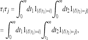
Now consider the case k = 2. For i > j we have simply

(13)

because the second indicator function vanishes when t₂ < t₁. Averaging over realizations we find

(14)

In deriving this result we used the multiplicative rule

(15)

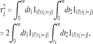
For i = j, by contrast, we find

(16)

which upon averaging yields

(17)

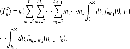
More general correlation functions are readily obtained in terms of multiple integrals over the functions f_nm. Inserting into (7) we see that the combinatorial factors (ν₂!)⁻¹ · · · (ν_n!)⁻¹ cancel to obtain

(18)

Equation 18 provides an explicit expression for the moments of the total branch lengths T_n in populations with population-size variations. The results can be written in a recursive form, particularly convenient for numerical computations,

(19)

with initial conditions for m ≥ 2 and for k ≥ 1. Here T_n(t) is the total time corresponding to the genealogy of n sequences sampled at time t in the past given a population-size curve x(t). Note that t = 0 corresponds to the present time, so that T_n(0) ≡ T_n. In a population of constant size, T_n(t) is independent of t.

Equation 18 or 19 expresses the kth moment of T_n in terms of a 2k-fold sum [according to (10) each factor of contains a sum over j_i]. Equation 18 can be further simplified by explicitly performing the sums over m₁, …, m_k. This results in

(20)

The coefficients are determined by recursion:

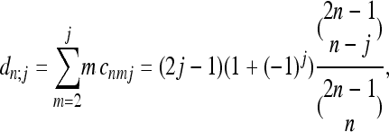(21)

(22)

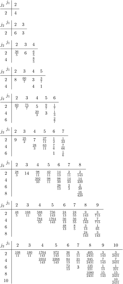
For the particular case k = 1 our result corresponds to an expression derived by Austerlitz et al. (1997) and Slatkin (1996) and also to the result obtained by summing Equation 1 in Zivkovic and Wiehe (2008). For k = 2, the coefficients are tabulated in Figure A1 in the appendix for small values of n. In general, the nested integrals in Equation 20 cannot be simplified further; their form expresses the correlations of the times τ_j due to population-size variations.

Figure A1.—

Coefficients occurring in Equation 20 for n = 2,…, 10. Coefficients for odd values of j₂ vanish.

Finally note that for n = 2, Equation 18 can be evaluated as follows:

(23)

This representation demonstrates how the expression (18) simplifies when k > n.

We conclude this section by briefly describing three different scenarios where our main result (Equation 18) is applicable. First, Sjödin et al. (2005) discussed a model where the scaled population size x(t) defined by Equation 3 may assume two values, 1 and x. The population size randomly jumps from 1 to x at rate λ and back at rate λ_x. Initially the population size is x(0) = 1. Our result (Equation 18) is directly applicable to a given realization of the random process x(t). We denote the ensemble average over realizations of x(t) by . By averaging Equation 18 over the corresponding distribution of Λ we find

(24)

Higher moments can be obtained in a similar fashion. This provides explicit expressions for the fluctuations of T_n in the case of slow, fast, and intermediate population-size changes. This model is particularly suited to examine the limit of fast population-size fluctuations . As expected, the standard Kingman coalescent, Equation 2, is recovered but now with an effective population size N_eff = N/c with c = (1 + x⁻¹)/2.

Second, intermediate population-size variations over many generations give rise to deviations from the standard Kingman behavior. The deviations are expected to be most significant when the timescale of the size variations is comparable to the times between coalescent events. Such intermediate population-size variations are commonly interpreted as due to a changing environment. In this case it is inappropriate to average over an ensemble of random population size curves x(t). The task is instead to describe the fluctuations of T_n conditional on a particular, externally imposed form of x(t). An example is the question: How does a recent bottleneck influence the distribution of T_n? To compute the kth moment of T_n, a k-fold integration is required. In general this must be performed numerically. However, in the case of piecewise constant functions x(t) the multiple integrals are straightforward to evaluate. If, on the other hand, the function x(t) is sufficiently “smooth,” the multiple integrals can be evaluated in closed form in the limits of slowly and rapidly varying population sizes as demonstrated below.

Third, in general stochastic population dynamics subject to a slowly changing environment may exhibit both slow changes due to an externally imposed change of the environment (in the form of a time-changing carrying capacity, for example) and “fast” (generation-to-generation) changes due to the random population dynamics. In the next two sections such a model is introduced and analyzed by means of Equation 18. The analysis is simplified by the observation that the fast size variations are irrelevant when their amplitude remains small. In this case Equation 18 may be evaluated using a deterministic population-size curve that is averaged over the fast changes. In the model discussed in the next two sections this curve is given by the deterministic time dependence of the carrying capacity.

A MODEL FOR A POPULATION WITH TIME-DEPENDENT CARRYING CAPACITY

The purpose of this section is to describe a modified Wright–Fisher model with a fluctuating carrying capacity. This model is used in the numerical simulations of sample genealogies described in the next section. Recall the three key assumptions of the Wright–Fisher model: (a) constant population size, (b) discrete, nonoverlapping generations, and (c) a symmetric multinomial distribution of family sizes. We have adopted the following approach: in our simulations, assumptions b and c are still satisfied, but assumption a is relaxed.

We study a large but finite population of fluctuating size N_l, where l = 1, 2,… labels the discrete, nonoverlapping generations forward in time. The model we have adopted is the following: consider a generation l consisting of N_l individuals. The number of individuals in generation l + 1 is then given by

(25)

where the random family sizes ξ_j are independent and identically distributed random variables having a Poisson distribution with parameter λ_l (specified below). Consequently the number N_l+1 is Poisson distributed with mean N_lλ_l.

This model exhibits a fluctuating population size N_l, rapidly changing from generation to generation. As pointed out in the Introduction, in large populations such fluctuations are averaged over by the ancestral coalescent process and can be captured in terms of an effective population size. The resulting genealogies are simply described by Kingman's coalescent for a constant effective population size of the form (1) or (4).

Interesting population-size fluctuations occur on larger timescales, corresponding to slow variations of the population size over several generations. Such slow changes are most commonly interpreted as consequences of a changing environment. A natural model for such changes is to impose a finite carrying capacity K_l that varies as a function of generation index l. This is the approach adopted in the following, and we choose

(26)

for a certain parameter value r > 0. Here K_l+1 is the carrying capacity in generation l + 1. If the environmental changes affected the population through fertility variations, K_l+1 would be replaced by K_l in Equation 26. Equation 26 is chosen so that the population ceases to grow on average when the carrying capacity is reached (λ_l = 1 for N_l = K_l+1). When the population size is small and , the population growth follows the logistic law, λ_l = 1 + r(1 − N_l/K_l+1), where r is the intrinsic growth rate. The particular form of Equation 26 ensures that λ_l > 0.

Note that fluctuations of N_l in this model are due to two different sources: rapid fluctuations are caused by the randomness of the family sizes, and slow fluctuations are caused by the time dependence of the carrying capacity. Our choice for the time dependence of K_l is dictated by the following considerations. The aim is to describe the influence of a fluctuating population size upon the statistics of genetic variation. To this end we need to consider the functional form of K_l. A simple choice for K_l is a periodically varying function, such as

(27)

Note that a more complex dependence of K_l upon l can be obtained from superpositions of such functions with different amplitudes ɛ and frequencies ν. Here we use simply (27) and investigate how the statistics of genetic variation in a sample depend upon frequency of the fluctuations in K_l.

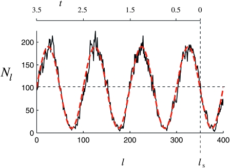
Figure 3 shows a realization of a curve N_l obtained in this manner (the choice of parameters is given in the Figure 3 legend). Figure 3 clearly exhibits fluctuations in N_l on two timescales, fast and slow. As explained above, the fast fluctuations are irrelevant provided their amplitude is sufficiently small. In this case we expect that the distribution of T_n can be described by a population-size curve that is averaged over the fast fluctuations. In the present model, averaging over the fast fluctuations results in a deterministic population-size curve determined by the carrying capacity (27). This curve is shown in Figure 3 as a dashed line.

Figure 3.—

One realization of the curve N_l obtained from simulations of the model described in a model for a population with time-dependent carrying capacity (black solid line). Choice of parameters: r = 1, K₀ = 100, ɛ = 0.9, and Nν = 1, with N = K₀. Also shown is an average over the fast fluctuations. The upper horizontal axis illustrates where the population is sampled and how time is counted backward in the coalescent approximation.

Note that conditional on the sequence of population sizes, the genealogy of a set of individuals sampled in generation l can be determined recursively by randomly choosing ancestors in the preceding generations. This is ensured by the assumption that, conditioned on the values of N_l and N_l+1, the family sizes follow a symmetric multinomial distribution . The resulting correspondence with the Wright–Fisher rule of reproduction ensures that the genealogies can be determined recursively in the way suggested above.

In the next section we analyze results of three sets of 10,000 computer simulations for this population model with parameters r = 1 and ɛ = 0.9 and for a range of values for ν. The three sets differ in the values for the average carrying capacity that are chosen to be K₀ = 100, K₀ = 1000, and K₀ = 10,000. The population is sampled in generation l_s (see Figure 3), which is chosen so that 2νl_s becomes an odd natural number. This implies that and that the population size was declining toward in the most recent past.

COMPARISON BETWEEN NUMERICAL SIMULATIONS AND COALESCENT PREDICTIONS

In this section we discuss the numerically computed distributions shown in Figure 2 in terms of Equation 18. The shapes observed in Figure 2 are conveniently characterized in terms of their mean , variance, skewness, and kurtosis:

(28)

(29)

Recall that for a normal distribution the skewness vanishes, and the kurtosis equals three. We can write the skewness and kurtosis in terms of the moments using

The moments are evaluated by means of Equations 18 and 19 as functionals of the scaled population size x(t) followed backward in time. With stochastically fluctuating sizes the scaled population size x(t) also becomes a random process. As Figure 3 indicates, the random fluctuations around the deterministic carrying capacity function are relatively small and we expect that such generation-to-generation fluctuations are irrelevant for the distribution of T_n. We therefore disregard the fast (random) fluctuations of the population sizes and define function x(t) deterministically by

(30)

This is obtained from an analog of Equation 3 when the population is sampled in generation l_s (as indicated in Figure 3):

(31)

Here (27) was used with ω = 2πνN, and N = K₀. Note that the particular form (30) of x(t) depends upon when the population is sampled. Had the population been sampled at a different time, a different curve x(t) could have resulted, leading in turn to a different distribution ρ(T_n) of T_n, since the distribution depends, for example, upon whether most recently the population was expanding or declining.

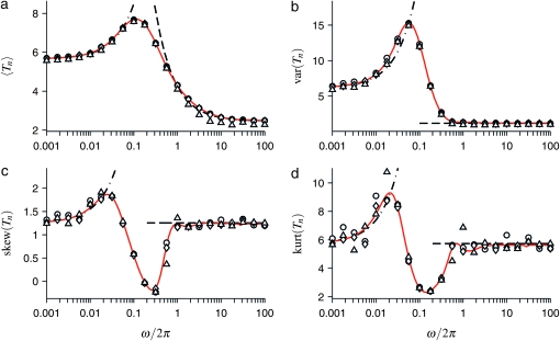
Our results are summarized in Figure 4. It shows how the mean, variance, skewness, and kurtosis of the distribution of T_n depend on the scaled frequency ω of the population size variation, Equation 30. Shown are results of numerical simulations of the model described in the previous section (symbols) and results obtained within the coalescent approximation using Equation 19. We observe that the coalescent approximation describes the results of the numerical simulations well, even for small population sizes.

Figure 4.—

Mean (a), variance (b), skewness (c), and kurtosis (d) of the distribution of T_n for samples of size n = 10, as a function of the frequency of the population-size fluctuations. Shown are results of numerical simulations (10,000 simulations with N = K₀, K₀ = 100, triangles; K₀ = 1000, diamonds; and K₀ = 10,000, circles) as well as results computed within the coalescent approximation described in coalescent approximation formulas for the moments (red solid lines). Black dashed-dotted and dashed lines show the approximations for small frequencies (Equations 33 and 34) and for large frequencies (Equations 39 and 40). The expressions for the limiting behaviors of the skewness and the kurtosis are shown in c and d, but are not given in the text. The remaining parameter values are r = 1 and ɛ = 0.9, as in Figure 2.

In the numerical simulations we have found that, for very small population sizes, random fluctuations of N_l around the time-dependent carrying capacity K_l become increasingly important. Since we suspected that the small deviations observed in Figure 4a for K₀ = 100 were due to such fluctuations, we performed slightly modified simulations imposing a deterministic law upon N_l by forcing N_l = K_l in every generation [where K_l is given by (27)]. Comparison of the corresponding results (not shown) with Figure 4a indicates that the deviations for K₀ = 100 at large frequencies are indeed caused by the stochastic fluctuations in the population dynamics underlying Figure 4a. A different interpretation of this effect is the following: when the population size is very small, and when ɛ is close to unity, the population may exhibit a nonnegligible probability of becoming extinct during the expected time to the most recent common ancestor for a sample of size n. In this case we have conditioned on the existence of the population during 100K₀ generations using rejection sampling. In practice this avoids extinction, but it leads to a biased size distribution.

Consider now the frequency dependence of the moments shown in Figure 4. It can be qualitatively and quantitatively understood using Equation 20 together with the following expression for Λ(t):

(32)

Here ⌈z⌉ is the smallest integer larger than z. Next we discuss the asymptotical formulas for small and large frequencies ω.

In the limit of , Equation 32 simplifies to . Inserting this into (20) we find approximately

(33)

Here and . Equation 33 is shown in Figure 4a as a dashed-dotted line. For the variance we find the approximate expression

(34)

with . The limiting value for zero frequency is that of the standard coalescent with constant population size. Equation 34 is shown in Figure 4b as a dashed-dotted line. Similarly the standard results for the constant-size coalescent are obtained for the skewness and for the kurtosis in the limit of . This limiting behavior is illustrated in Figure 2a, which shows that the distribution of T_n approaches that for Kingman's coalescent for a constant population size in the limit of small frequencies. We note that for , the population-size dependence is essentially that of a declining population, because the time to the most recent common ancestor is reached before the first maximum in x(t) going backward in time (see Figure 3 and Equation 30).

Of particular interest is the limit of large frequencies, as we now show. As ω→∞, one expects that the coalescent process averages over the population-size oscillations, and the standard coalescent process with a constant effective population size should be obtained. For large but finite frequencies, by contrast, Figure 4a exhibits deviations from the standard coalescent behavior. In the following we analyze the behavior of the moments in this regime. In the limit of large frequencies, Equation 32 simplifies to

(35)

For large frequencies, the function Λ(t) is well approximated by a shifted linear function

(36)

Here c determines the effective population size according to Equation 4: N_eff = N/c with

(37)

The parameter c describes the influence of the demographic fluctuations upon the part of the genealogy in the distant past. The small offset

(38)

describes the influence of demographic changes on the most recent part of the genealogy. Inserting the approximation (36) into (20) we find for large frequencies (and when the amplitude ɛ is not too close to unity)

(39)

The first term in (39) is the expected time of Kingman's coalescent for a constant effective population size N_eff = N/c. The curve corresponding to (39) is shown as a dashed line in Figure 4a. We infer that corrections to the standard coalescent result are significant when the sample size is large, the amplitude of the size oscillations is not too small, and the frequency ω is of order unity. This is consistent with the results of Sjödin et al. (2005).

We now discuss the behavior of the variance shown in Figure 4b. For the second moment we find

(40)

The first term in Equation 40 corresponds to the second moment of T_n in Kingman's coalescent with a constant effective population size. The second term in (40) represents a correction due to finite but large frequencies; it depends in a simple fashion on the effective population-size parameter c and on the sample size n.

Comparing Equations 39 and 40, we arrive at the conclusion that the corresponding correction for the variance var(T_n) vanishes. This is consistent with the fact that, at large frequencies, the variance of T_n is surprisingly insensitive to changes in frequency (as opposed to the behavior of , see Figure 4, a and b). In fact, the limiting value (shown in Figure 4b as a dashed line) is a very good approximation to var(T_n) down to ω ≈ 3.

Consider now the skewness and the kurtosis shown in Figure 4, c and d. Their behavior is similar to that of the variance: for ω > 3, the skewness and the kurtosis are essentially independent of ω. The results shown in Figure 4 imply that over a large range of frequencies, the distribution of the total branch lengths T_n can be approximated as follows: the distribution is essentially that of the standard Kingman coalescent with an effective population size, but the distribution is shifted such that its mean is given by Equation 39, rather than by 2h_n/c.

One may wonder when this “rigid shift” occurs. Given Equation 18 it is straightforward to work out the fluctuations of the times τ_j within the approximation (36). We find that for j < n, the expected value of τ_j is exactly that of the standard Kingman coalescent with effective population size. But for j = n it is rigidly shifted by −Λ₀/c. This indicates that the genealogies are essentially those of the standard coalescent, but modified by an initial rigid shift. In the parameter regime discussed here, the distribution of times is expected to be well approximated by a two-parameter family of distributions,

(41)

when zc > −nΛ₀, and P(T_n < z) ≈ 0 for smaller values of z. The first parameter determines the effective population size. It parameterizes the slope of the function Λ(t) at large times and describes the demographic effect on the distant past of the genealogy. The second parameter, Λ₀ describes the influence of the demographic fluctuations on the initial part of the sample genealogy. This parameter can be negative (recent population decline, this is the case shown in Figure 3) or positive (recent population expansion). When Λ₀ > 0, the distribution ρ(T_n) is rigidly shifted to the left. In this case the approximation (36) is expected to break down when the body of the distribution reaches T_n = 0.

Note that the distribution (41) cannot be described by a single parameter (a “generalized effective population size”). The approximation (41) was used to generate the red dashed curve in Figure 2d.

CONCLUSIONS

The aim of this article was to investigate how the frequency of population-size fluctuations determines the shape of the distribution of total branch lengths of sample genealogies and thus of statistical measures of genetic variation.

We performed simulations for a modified Wright–Fisher model of a population subject to a time-periodically varying carrying capacity and determined the distribution of the total branch lengths, shown in Figure 2. We characterized how the shapes of the distributions depend upon the frequency of the population-size fluctuations by computing the frequency dependence of the moments of these distributions. We could explain these dependencies in terms of coalescent approximations. In particular, we derived a general expression—Equation 20—for the moments in populations subject to smooth population changes of otherwise arbitrary form.

Our results show how quickly (or slowly) the standard coalescent result for a constant (effective) population sizes is recovered in the limits of large and small frequencies. More importantly, our coalescent results allow us to determine how significant deviations are at large but finite frequencies. In this case we argued that at large frequencies, the distribution of T_n is essentially that of the standard Kingman coalescent with an effective population size N_eff = N/c, but with a shifted mean value

(42)

The first term on the rhs corresponds to the result of the standard Kingman coalescent with a constant effective population size. The second term on the rhs is the correction term resulting from the population-size variations (ɛ is the amplitude of the population-size oscillations, ω is its frequency, and n is the sample size). We infer that corrections to the standard coalescent result are largest when the sample size is large and the amplitude ɛ of the size fluctuations is not very small. This is consistent with the results of Sjödin et al. (2005).

Last but not least we found that the coalescent approximation yields a reliable description of the numerical data, even for very small populations.

We close with a number of remarks. First, Equation 20 is easily generalized to describe the moments of observables that are polynomial functions of the times τ_j. Particularly simple is the case of observables A that are linear functions of the times τ_j, . In this case the kth moment of A_n is given by Equation 20, but with modified coefficients: the factors m in Equations 21 and 22 are replaced by a_m.

Second, some observables [such as the F-statistic (Fu and Li 1993)] can be written as linear functions of τ_j, but with random coefficients. In this case too it is possible to explicitly compute the moments of the distribution of the observable. These two questions are addressed in a separate article (S. Sagitov, M. Rafajlovic, B. Mehlig, and A. Eriksson, unpublished results).

Third, Equation 19 allows us to determine in a transparent fashion how the fluctuations of T_n depend upon the time at which the population is sampled. This will make it possible to discuss, for example, how Tajima's D-statistic or the F-statistic depends upon the time of sampling after a bottleneck, a population expansion, or a decline.

Fourth, population-size fluctuations are sampled nonuniformly by the genealogies: initial coalescent events occur at faster rates and are thus more sensitive to recent size fluctuations. Remote coalescent events, by contrast, occur at slower rates, thus damping the effect of size fluctuations in the distant past. We therefore expect significant deviations from the standard coalescent behavior arising from the most recent history for large sample sizes n. It would be interesting to quantify this expectation by computing the covariances and higher moments of the times τ_j during which the sample genealogy has j lines: first, for large i ≈ n and j ≈ n we expect to observe strong correlations between τ_i and τ_j and thus deviations from the standard Kingman coalescent. Second, for small values of i and j we expect the times τ_i and τ_j to decorrelate and to follow the distribution of the standard coalescent (with an effective population size).

Fifth, the model introduced in a model for a population with time-dependent carrying capacity assumes a carrying capacity that varies sinusoidally, with a single frequency. It turns out, however, that our findings (summarized in Equation 41) are valid for arbitrary time-dependent fluctuations with a sufficiently strong and narrow mode at high frequencies. Examples are linear combinations of high-frequency oscillations or stochastic fluctuations around a constant population size, with a sufficiently narrow frequency spectrum. In this case, too, we expect that Λ(t) is well approximated by (36). If this is the case, the distribution of times is of the form (41) when Λ₀ is small.

Taken together, the results derived in this article give a rather complete understanding of the fluctuations of empirical observables due to population size variations. These results will be significant when attempting to disentangle the effects of population-size variations from other factors influencing genetic variation.

Our results raise the question under which circumstances the deviations from standard coalescent behaviors due to population-size fluctuations (Figures 2 and 4) are most likely to strongly affect the interpretation of empirical data. As our analysis indicates, the deviations become substantial when the frequency ω = 2πνN is of order unity. Here ν is the frequency of the population size variations, Equation 30, and N is a suitable measure of the population size. In other words, rapid population-size fluctuations will have the strongest effect (other than simply determining the effective population size) in small local subpopulations with restricted gene flow between subpopulations with different fluctuations. The deviations are expected to be smaller at larger spatial scales, because the ancestral process averages over the spatial fluctuations. More generally, we conclude that deviations from standard coalescent behavior are expected for populations subject to an environment that changes as a function of space and time on neither too small nor too large length and timescales. An example for such a population is the marine snail Littorina saxatilis. Its habitat on the Northern coast of Bohuslän (Sweden) is fragmented into subpopulations with strongly restricted gene flow between them, and effective population sizes of subpopulations have been found to be very small (K. Johannesson, personal communication). Starting from the results derived in this article, we hope to determine gene genealogies in such fragmented populations subject to variations of population size in space and time.

APPENDIX: COEFFICIENTS FOR n = 2,…, 10

In Figure A1 we give the coefficients determining the second moment according to Equation 20 for n = 2,…, 10. Note that the coefficient for n = 2 is consistent with Equation 23.

References

- Austerlitz, B., B. Jung-Muller, B. Godelle and P. Gouyon, 1997. Evolution of coalescence times, genetic diversity and structure during colonization. Theor. Popul. Biol. 51 148–164. [Google Scholar]
- Ewens, W., 1982. The concept of the effective population size. Theor. Popul. Biol. 21 373–378. [Google Scholar]
- Fisher, R. A., 1930. The Genetical Theory of Natural Selection. Clarendon Press, Oxford.
- Fu, Y., and W. Li, 1993. Statistical tests of neutrality of mutations. Genetics 133 693–709. [DOI] [PMC free article] [PubMed] [Google Scholar]
- Garrigan, D., and M. F. Hammer, 2006. Reconstructing human origins in the genomic era. Nat. Rev. Genet. 7 669–680. [DOI] [PubMed] [Google Scholar]
- Griffiths, R., and S. Tavaré, 1994. Sampling theory for neutral alleles in a varying environment. Philos. Trans. R. Soc. Lond. B 344 403–410. [DOI] [PubMed] [Google Scholar]
- Hein, J., M. H. Schierup and C. Wiuf, 2005. Gene Genealogies, Variation and Evolution: A Primer in Coalescent Theory. Oxford University Press, London/New York/Oxford.
- Jagers, P., and S. Sagitov, 2004. Convergence to the coalescent in populations of substantially varying size. J. Appl. Probab. 41 368–378. [Google Scholar]
- Kaj, I., and S. Krone, 2003. The coalescent process in a population with stochastically varying size. J. Appl. Probab. 40 33–48. [Google Scholar]
- Kingman, J., 1982. The coalescent. Stoch. Proc. Appl. 13 235–248. [Google Scholar]
- Moran, P., 1958. Random processes in genetics. Proc. Camb. Philos. Soc. 54 60–71. [Google Scholar]
- Nordborg, M., and S. Krone, 2003. Modern Developments in Population Genetics: The Legacy of Gustave Malécot, pp. 194–232. Oxford University Press, Oxford.
- Sjödin, P., I. Kaj, S. Krone, M. Lascoux and M. Nordborg, 2005. On the meaning and existence of an effective population size. Genetics 169 1061–1070. [DOI] [PMC free article] [PubMed] [Google Scholar]
- Slatkin, M., 1996. Gene genealogies within mutant allelic classes. Genetics 143 579–587. [DOI] [PMC free article] [PubMed] [Google Scholar]
- Tajima, F., 1989. Statistical method for testing the neutral mutation hypothesis by DNA polymorphism. Genetics 123 585–595. [DOI] [PMC free article] [PubMed] [Google Scholar]
- Tavaré, S., 1984. Lines of descent and genealogical processes, and their application in population genetics models. Theor. Popul. Biol. 26 119–164. [DOI] [PubMed] [Google Scholar]
- Tavaré, S., 2004. Ancestral Inference in Population Genetics, pp. 1–188. Springer, Berlin.
- Wakeley, J., and O. Sargsyan, 2009. Extensions of the coalescent effective population size. Genetics 181 341–345. [DOI] [PMC free article] [PubMed] [Google Scholar]
- Wright, S., 1931. Evolution in Mendelian populations. Genetics 16 97–159. [DOI] [PMC free article] [PubMed] [Google Scholar]
- Zeng, K., Y. Fu, S. Shi and C. Wu, 2006. Statistical tests for detecting positive selection by utilizing high-frequency variants. Genetics 174 1431–1439. [DOI] [PMC free article] [PubMed] [Google Scholar]
- Zivkovic, D., and T. Wiehe, 2008. Second-order moments of segregating sites under variable population size. Genetics 180 341–357. [DOI] [PMC free article] [PubMed] [Google Scholar]