Spatial HARDI: Improved Visualization of Complex White Matter Architecture with Bayesian Spatial Regularization

Abstract

Imaging of water diffusion using magnetic resonance imaging has become an important noninvasive method for probing the white matter connectivity of the human brain for scientific and clinical studies. Current methods such as diffusion tensor imaging (DTI), high angular resolution diffusion imaging (HARDI) such as q-ball imaging, and diffusion spectrum imaging (DSI), are limited by low spatial resolution, long scan times, and low signal-to-noise ratio (SNR). These methods fundamentally perform reconstruction on a voxel-by-voxel level, effectively discarding the natural coherence of the data at different points in space. This paper attempts to overcome these tradeoffs by using spatial information to constrain the reconstruction from raw diffusion MRI data, and thereby improve angular resolution and noise tolerance. Spatial constraints are specified in terms of a prior probability distribution, which is then incorporated in a Bayesian reconstruction formulation. By taking the log of the resulting posterior distribution, optimal Bayesian reconstruction is reduced to a cost minimization problem. The minimization is solved using a new iterative algorithm based on successive least squares quadratic descent. Simulation studies and in vivo results are presented which indicate significant gains in terms of higher angular resolution of diffusion orientation distribution functions, better separation of crossing fibers, and improved reconstruction SNR over the same HARDI method, spherical harmonic q-ball imaging, without spatial regularization. Preliminary data also indicate that the proposed method might be better at maintaining accurate ODFs for smaller numbers of diffusion-weighted acquisition directions (hence faster scans) compared to conventional methods. Possible impacts of this work include improved evaluation of white matter microstructural integrity in regions of crossing fibers and higher spatial and angular resolution for more accurate tractography.

INTRODUCTION

Diffusion MRI has rapidly become an important noninvasive tool for characterization of white matter structure because it enables the visualization and evaluation of fiber tracts connecting cortical regions. Clinical uses range from the evaluation of white matter fiber microstructural integrity due to neurodegeneration, traumatic injury, or primary demyelinating white matter diseases such as multiple sclerosis to 3D tractography for neurosurgical planning. The most commonly used technique, diffusion tensor imaging (DTI), resolves water diffusion in terms of cardinal ellipsoidal shapes, ranging from purely spherical in the absence of oriented fibers to prolate ellipsoids in the presence of healthy fibers predominantly oriented along a single direction (Beaulieu, 2002).

While the diffusion tensor can be estimated from as few as 6 different diffusion directions, it suffers from the important limitation that it cannot resolve individual orientations within voxels that contain fibers with more than one orientation. As a result, it is difficult to resolve crossing fibers and to accurately perform tractography in these areas of complex fiber architecture. High angular resolution diffusion imaging (HARDI) techniques overcome this limitation of DTI by measuring diffusion attenuation in many more angular directions, typically dozens or even hundreds, in order to resolve the orientations of multiple fiber populations co-existing in the same voxel. Compared to DTI, HARDI can faithfully reproduce underlying complex fiber geometries by better resolving the angular dependence of intravoxel diffusion. DTI is a limited SNR and low spatial resolution modality compared to routine clinical T1- and T2-weighted MR imaging. Because it employs higher diffusion-weighting factors (b-values), HARDI yields even lower SNR than DTI. Furthermore, it requires longer experiment times to acquire many diffusion directions, thus reducing practical feasibility for routine clinical neuroimaging. Further reduction in scan time is possible in HARDI only at the cost of lower SNR and/or angular resolution.

The goal in HARDI is to construct the fiber orientation distribution function (ODF) F(u) (Tuch, 2002), a spherical function that characterizes the relative likelihood of water diffusion along any given angular direction u. Several approaches have been proposed to recover F(u) from raw diffusion-weighted data, including spherical harmonic modeling of the apparent diffusion coefficient (ADC) profile (Frank, 2002; Alexander et al., 2002), multitensor modeling (Tuch, et al., 2002), generalized tensor representations (Ozarslan et al., 2003; Liu et al., 2004), circular spectrum mapping (Zhan et al., 2004), q-ball imaging (QBI) (Tuch, 2004; Tuch, 2005; Hess et al., 2006; Mukherjee et al., 2007), persistent angular structure (Jansons et al., 2003), spherical deconvolution (Tournier et al., 2004), and diffusion orientation transform (DOT) (Ozarslan et al, 2006). In this paper, we focus on QBI due to its linearity, model independence and sensitivity to multimodal diffusion; in fact the correspondence between QBI ODF peaks and multimodal fiber orientations has been established using phantom models (Perrin et al., 2005). Recently, improved results have been reported using a spherical harmonic representation (Groemer, 1996) for QBI (shQBI) (Anderson, 2005; Hess et al., 2006; Descoteaux et al., 2007). The use of a spherical harmonic basis is parsimonious for typical b-values, which enables the ODF to be synthesized from a relatively small number of noisy measurements and thus brings the technique closer to clinical feasibility from the standpoint of total imaging time. The presented work is based upon this parsimonious shQBI approach.

Proposed Method

We aim to improve the shQBI reconstruction from diffusion MRI data by exploiting a priori knowledge about the smoothly varying orientation structure of white matter tracts over 3D space and incorporating this knowledge as a constraint in the reconstruction. This approach, which we call spatially coherent HARDI, or “spatial HARDI” for short, improves noise tolerance, spatial resolution, and fiber orientation accuracy compared to conventional methods. It is important to note that, although the presented work applies to shQBI, it can be equally well applied to other QBI reconstruction methods. As DTI can be considered as a special case of HARDI at lower angular resolution, this new technique would also be applicable to both conventional DTI and more recently developed HARDI methods including spherical deconvolution and DOT.

With the proposed method, spatial smoothness constraints are determined from the neighborhood of each voxel and incorporated into the HARDI reconstruction algorithm. The motivation for this approach is that the angular variability of the diffusion function in HARDI is expected to be spatially coherent within any given white matter tract. In other words, the orientation and anisotropy of any single fiber population are expected to change smoothly from one voxel to the next, particularly along the dominant fiber orientation, except at the boundaries between tracts and interfaces with gray matter structures and cerebrospinal fluid (CSF) spaces. This a priori assumption constitutes a very important and powerful constraint that can be exploited to improve the conditioning and therefore the noise tolerance of the reconstruction step. Current techniques do not make use of this spatial constraint because they perform the reconstruction independently for each voxel. In this paper, we develop the mathematical framework necessary to incorporate spatial smoothness as a constraint and jointly estimate the HARDI reconstruction parameters for each voxel in the entire volume simultaneously. We explore spatial prior models incorporating global and directional smoothness constraints, described in the Theory section. Spatial constraints are specified in terms of a prior probability distribution, which is then incorporated in a Bayesian formulation of the reconstruction problem. By taking the log of the resulting posterior distribution, the reconstruction problem is reduced to a cost minimization. The minimization is solved using a new iterative algorithm based on least squares Q-R (LSQR) iterations (Paige et al., 1982), which accommodates non-convex and data-dependent terms in the cost function. We show that, by incorporating non-linear weight updates in our proposed algorithm within the LSQR iteration, execution time of our approach can be made linear in the number of voxels. Testing and validation of the technique using simulations as well as in vivo HARDI data are reported in the Results section.

Related Work

Resolving ODFs from available diffusion directions under noise and scan time limitations is a well-studied subject in the field of diffusion MR; here we review only recent work most relevant to our study. Deterministic (Tuch, 2002; Hess et al., 2006; Tournier et al., 2004; Descoteaux et al., 2007; Sakaie et al., 2006) as well as probabilistic (Jian et al., 2007; Tristan-Vega et al., 2009) approaches have been proposed.

Tournier et al. (2004) proposed a spherical deconvolution approach to obtaining the ODFs from raw diffusion data. Tristan-Vega et al. (2009) proposed a probabilistic method for computing the orientation probability density function, and demonstrated improved results over traditional Q-ball reconstruction using spherical harmonics. Estimation of spherical harmonic coefficients in a manner very similar to the work of Hess et al., (2006), but incorporating a different regularization term using Laplace-Beltrami operators, was proposed in (Sakaie et al., 2006, Descoteaux et al. 2007). This regularization method was shown to perform better than the traditional Tikhonov regularization proposed by Hess et al.

Although our work uses spherical harmonic functions as the ODF model, many other models have been proposed and fruitfully employed in the field. The “persistent angular structure”, or PASMRI, method was proposed by Jansons et al., (2003) as a nonlinear parametric technique for orientation estimation. A multi-tensor model proposed (Hosey et al., 2005; Tuch, 2002) appears to reliably capture mixed fiber populations; this model was solved by Hosey et al. (2005) in a probabilistic Bayesian manner and produced estimates of the number of fibers in each voxel. A tensor distribution model was employed by Jian et al., (2007) where the mixture distribution was modeled as a Wishart distribution. Other models include the original radial basis function q-ball model of Tuch (2004). The present work differs from existing methods in that our focus is not on the particular ODF reconstruction method, but rather on a powerful framework for spatially-constrained joint ODF estimation; our approach can be equally well employed on any of these other ODF models.

Our method is also related to the literature on denoising of HARDI ODFs, for which several methods have been proposed (Kim et al., 2009; Goh et al., 2009). Kim et al. (2009) proposed a variational approach, and Goh et al. (2009) proposed denoising in the framework of convolution operations on a derived Riemannian manifold. Especially the latter work is in many ways the correct one for diffusion ODFs, and would appear the right model for denoising and other post-processing operations. Denoising the raw diffusion images first, followed by reconstruction has also been proposed (Descoteaux et al., 2008). These denoising methods are not directly comparable to our work, because we wish to both reconstruct and denoise the ODFs at the same time, instead of first reconstructing and then denoising, or denoising then reconstructing.

To summarize, existing methods have either focused on developing new models for single voxel ODFs using various basis functions, or on statistically optimal estimation of model parameters under constraints on single voxel ODFs. To our knowledge, the proposed approach is the first one advocating the joint estimation of ODFs across the image, using spatial constraints to simultaneously regularize and denoise the problem. Spatial regularization has previously been performed for smoothing or denoising as a post-processing step, but not as an integral part of the ODF reconstruction process itself.

THEORY AND BACKGROUND

Q-Ball Imaging Using Spherical Harmonic Reconstruction

According to the q-space formalism, the wavevector that describes diffusion encoding in a pulsed-gradient spin-echo experiment is defined as q = (2π)⁻¹γδg, where γ represents the gyromagnetic ratio, δ is the diffusion gradient duration, and g is the diffusion gradient vector. HARDI acquisition schemes measure samples from an underlying diffusion-attenuated signal E(q) at a finite set of points on the sphere that are relatively uniform in their angular distribution. The choice of the spherical sampling radius in q-space, q₀, depends on the desired angular resolution, the available SNR, and the gradient performance specifications. In practice, b-values of 3000 s/mm² or greater are typically required in order to distinguish among different intravoxel fiber populations at high angular resolution (Hess et al., 2006).

To simplify the numerical solution, both q and u are discretized to reflect finite sampling of m measurements and reconstruction over a fixed number of points n. Because both the ODF and the diffusion signal are defined on the domain of the sphere, it is convenient to normalize spherical points to unit magnitude and adopt a spherical coordinate system q = q(θ,φ) and u = u(θ,φ), where θ and φ denote elevation and azimuth, respectively.

Linear HARDI reconstruction algorithms such as QBI and spherical deconvolution have in common that each point of the reconstruction is computed as a linear combination of the diffusion measurements. Enumerating points on the sphere to construct a vector representation, this relationship can be expressed as

$$\mathbf{e}={\mathbf{Z}}_Q\mathbf{P}{\mathbf{Z}}_U^{†}\mathbf{f}$$

where f and e denote n × 1 and m × 1 column vectors composed of the estimated values of the ODF and the diffusion measurements, respectively. Here Z_Q is the matrix of spherical harmonics evaluated at measurement points Q, and Z_U is the matrix of spherical harmonics evaluated at reconstruction points U. Diagonal matrix P = diag[p₀, p₂,…, p_L] contains the Legendre polynomials of order l = 0, 2,…, L. Details of notation and formulation are contained in Hess et al., (2006). The conventional way of obtaining an estimate of f given e is the pseudoinverse, which happens to be the maximum likelihood estimator in the presence of Gaussian additive noise:

$$\begin{array}{l}\mathbf{f}=\mathbf{Ae},\\ \mathbf{A}={\mathbf{Z}}_U{\mathbf{P}}^{-1}{\mathbf{Z}}_Q^{†}(\mathit{pseudoinverse})\\ \mathbf{A}={\mathbf{Z}}_U{\mathbf{P}}^{-1}{({\mathbf{Z}}_Q^H{\mathbf{Z}}_Q+\mu I)}^{-1}{\mathbf{Z}}_Q^H(\mathit{Tikonov}\mathit{regularization})\end{array}$$

Depending on the reconstruction algorithm employed, the n × m reconstruction matrix A is constructed using the spherical sampling geometry and the assumed relationship between the diffusion space and the ODF. The ODF was obtained by Hess et al., (2006) in two ways – first by direct pseudoinverse of A as above, and also by adding a standard Tikhonov regularization term. Tikhonov regularization (Press et al., 1992) is performed to reduce the noise sensitivity of the transform. The harmonic q-ball reconstruction in both cases is a linear transform of the diffusion measurements. Because the spherical harmonics form a complete spherical basis, the representation is capable of describing any bounded, finite-energy ODF given a sufficiently large order L.

A New Bayesian ODF Reconstruction Algorithm Exploiting Spatial Priors

We now use a Bayesian estimation framework to introduce spatial smoothness constraints during the reconstruction. Our motivation is that voxels in diffusion images are expected to be coherent, both along spatial dimensions and in diffusion orientation space. Except at the boundaries between tracts, the density, orientation and anisotropy of fiber populations are expected to change smoothly from one voxel to the next, particularly along the dominant fiber orientation. For instance, the circled fibers in Figure 1 can be seen to belong to the same bundle, and hence among the voxels that contain fibers from this tract, there is a strong spatial coherence. These constraints can be exploited to improve the numerical conditioning of the reconstruction, and thereby decrease the sensitivity to noise. Current techniques do not make use of these constraints because they perform the ODF reconstruction independently for each voxel.

Figure 1.

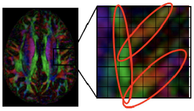
Spatial and angular coherence in HARDI. Except at the boundaries between separate tracts, fiber orientation in neighboring voxels varies smoothly, and as a result adjacent voxels are likely to have similar ODFs. By imposing spatial constraints among individual fiber tracts, it is possible to mitigate noise and other limitations.

To incorporate smoothness constraints and to jointly estimate the ODFs of each voxel within the entire volume, we cast the problem of estimating the parameters of all HARDI ODFs together as one of minimization of a cost function that incorporates the probabilistic spatial constraints.

Suppose Z_Q, Z_U, P etc are defined as before, and let us capture, in vector η all the spherical harmonic coefficients of the entire spatial field, and in vector f, the corresponding ODF field. For voxels enumerated as 1, …, p, …, N, this defines a collection of individual voxel-wise coefficients and ODFs:

$$\begin{array}{l}\mathbf{\eta }={[{{\mathbf{\eta }}^T}_1,\text{L},{{\mathbf{\eta }}^T}_p,\text{L},{{\mathbf{\eta }}^T}_N]}^T,\\ \mathbf{f}={[{{\mathbf{f}}^T}_1,\text{L},{{\mathbf{f}}^T}_p,\text{L},{{\mathbf{f}}^T}_N]}^T\end{array}$$

The task is then to estimate the value of η that simultaneously (1) fits both the diffusion measurements within each voxel (data consistency), and (2) minimizes the smoothness cost function that encodes inter-voxel spatial constraints. Since the estimation is jointly over all voxels, it is convenient mathematically to concatenate matrices Z_Q, Z_U, P diagonally, yielding matrices that operate on all the voxels, as follows:

$${\overline{\mathbf{Z}}}_Q=\left[\begin{array}{ccc}{\mathbf{Z}}_Q& & \\ & \ddots & \\ & & {\mathbf{Z}}_Q\end{array}\right],{\overline{\mathbf{Z}}}_U=\left[\begin{array}{ccc}{\mathbf{Z}}_U& & \\ & \ddots & \\ & & {\mathbf{Z}}_U\end{array}\right],\overline{\mathbf{P}}=\left[\begin{array}{ccc}\mathbf{P}& & \\ & \ddots & \\ & & \mathbf{P}\end{array}\right]$$

Assuming uncorrelated Gaussian additive noise, the likelihood function is given by

$$Pr(e\mid \eta )\propto e^{-\alpha {\left|\right|e-\overline{P}{\overline{Z}}_Q\eta \left|\right|}^2}$$ (1)

The constant α is inversely related to the power of additive noise and is assumed to be an unknown quantity to be estimated empirically. For spatial constraints, we employ the following probability distribution model:

$$Pr(\mathbf{\eta })\propto {\mathbf{e}}^{-{\beta }_1{\left|\right|\mathbf{DW}(\mathbf{\eta })\mathbf{\eta }\left|\right|}^2}·{\mathbf{e}}^{-{\beta }_2\left|\right|\mathbf{\eta }\left|\right|{\mathbf{R}}^2}$$ (2)

where subscript R is shorthand for vector norm with respect to some matrix $\mathbf{R}:{\left|\right|\mathbf{x}\left|\right|}_{\mathit{R}}\triangleq {\mathbf{x}}^{\mathit{H}}\mathbf{Rx}$. Scalars β₁ and β₂ are unknown constants, called hyperparameters of the prior distribution (2), which are empirically determined as described in Methods section, matrix D is a first difference operator, and W(η) is a matrix that represents a neighborhood weighting function. Here we have omitted the partition function for tractability. We will allow the weight matrix to depend on the configuration of ODFs, hence it is shown as parameterized by η The motivation behind this prior model is discussed below. We note that recently so-called robust priors involving the L₁ norm have been proposed in related fields (Raj et. al, 2007) but we eschew that approach for reasons of computational complexity.

In Bayesian methods, the task is to find the unknown configuration η, given observations e and knowledge of likelihood and prior probability distributions. Here we use the maximum a posteriori (MAP) estimator, which selects the η that maximizes the posterior probability

$$Pr(\mathbf{\eta }\mid \mathbf{e})\propto Pr(\mathbf{e}\mid \mathbf{\eta })Pr(\mathbf{\eta })$$ (3)

which follows from Bayes’ Theorem. Combining the above equation with the negative log of Eqns (1) and (2), the MAP estimate can be obtained by minimization of the cost function:

$$\stackrel{⌢}{\mathbf{\eta }}={\text{argmin}}_{\mathbf{\eta }}\left\{{\left|\right|\mathbf{e}-\overline{\mathbf{P}}{\overline{\mathbf{Z}}}_Q\mathbf{\eta }\left|\right|}^2+{\lambda }^2{\left|\right|\mathbf{DW}(\mathbf{\eta })\mathbf{\eta }\left|\right|}^2+{\mu }^2{{\left|\right|\mathbf{\eta }\left|\right|}_{\mathbf{R}}}^2\right\}$$ (4)

where $\lambda =\frac{{\beta }_1}{\alpha },\mu =\frac{{\beta }_2}{\alpha }$ are unknown constants, which can be interpreted as regularization factors whose heuristic determination is described in Methods section. From the MAP estimate of the spherical harmonic coefficients η, the ODF profile is computed voxelwise according to

$$\stackrel{⌢}{\mathbf{f}}={\overline{\mathbf{Z}}}_{\text{U}}\stackrel{⌢}{\mathbf{\eta }}$$ (5)

This Bayesian formulation of ODF reconstruction has similarities with regularized reconstruction methods proposed earlier, especially Tikhonov regularization. The first term in Eq. (4) can be understood to enforce data consistency and exactly reproduces the least squares fitting approach. The last term enforces Tikhonov regularization (when R=I) by adding a stabilizing term to the least squares fitting and favors solutions which have a low L₂ norm. As mentioned above, there exists an explicit formula for computing this estimate using the Moore-Penrose pseudoinverse. Although we show the Tikhonov regularization term, our work is independent of which regularization scheme is used – whether Tikhonov, Laplace-Beltrami or otherwise. For brevity these other terms are not shown, but we assume that they can be captured by an appropriate norm induced by matrix R. The middle term is new, and introduces the spatial smoothness cost discussed above. When W(η) = I, the solution that results is maximally smooth under the data consistency constraint, because other potential non-smooth solutions will have a large first derivative norm and cause the smoothness cost to increase.

While global smoothness is frequently used in multi-dimensional imaging applications, its utility is limited in situations where global smoothness may not apply. For instance, the ODF field in typical MR data displays smoothness along the orientations of individual fiber bundles but may not display smoothness perpendicular to the fiber, or around voxels with crossing fibers. Global smoothness in these situations may lead to an indiscriminate blurring of the ODFs. To prevent this from occurring, we use a spatial weight matrix W(η). This matrix determines the strength of the constraint to place on the similarity of the spherical harmonics between neighboring voxels. Because the weight between two neighboring voxels should generally depend on their ODFs and hence on the joint configuration η, we denote an explicit dependence on η. Computationally, the nonlinearity that the spatial weighting matrix introduces into the function renders the optimization sensitive to starting estimates and prone getting stuck in local minima. Ideally the estimation of η should reflect the non-linear presence of W; however the resulting estimation problem would then become intractable and difficult to minimize.

Here we propose a simple iterative scheme whereby both W(η) and η are updated alternately. The process is summarized below:

• Begin with η = η₀. Then for k = 1 to K, repeat:

  1. Form W^k(η) = [w_p,q] ∀ (p,q) ε , where $w_{p,q}=1-\frac{\left|\right|{{\eta }_p}^k-{{\eta }_q}^k\left|\right|}{\left|\right|{{\eta }_p}^k\left|\right|\left|\right|{{\eta }_q}^k\left|\right|}$

  2. Form $\overline{{\mathbf{A}}^k}=\left(\begin{array}{c}\overline{\mathbf{P}}{\overline{\mathbf{Z}}}_{\text{Q}}\\ \lambda \mathbf{DW}({\mathbf{\eta }}^k)\\ \mu \mathbf{R}\end{array}\right),\overline{\mathbf{e}}=\left(\begin{array}{c}\mathbf{e}\\ \mathbf{0}\\ \mathbf{0}\end{array}\right)$

  3. Solve $\widehat{{\mathbf{\eta }}^{\text{k}}}={\text{argmin}}_{\mathbf{\eta }}\left\{{\left|\right|\overline{\mathbf{e}}-\overline{{\mathbf{A}}^k}\mathbf{\eta }\left|\right|}^2\right\}$ using LSQR algorithm (Paige, et. al., 1982)

• Finally, reconstruct ODF: f̂ = Z̄_Uη̄^K̄

Here refers to the 3D neighborhood system corresponding to the 26 nearest neighbors of every voxel. This iterative update algorithm alternately estimates the spatial weight matrix based on the current estimate of the ODF field, and then applies this weight matrix to solve for the Bayesian estimator. The initial estimate is based on the unconstrained ODF estimate obtained for each voxel.

The ODF field estimate is iteratively refined by minimizing the cost function in Eq. 5, using a least squares algorithm called LSQR (Paige, et. al., 1982), which is based on conjugate gradient descent. Because the cost function passed to LSQR is a quadratic function, it can be easily calculated. We employed the LSQR implementation in MATLAB version 7.8.0. LSQR was chosen for this purpose for several reasons. First, in each iteration, step 3 above is a linear least squares problem, which is preferable to solving an unconstrained general optimization problem. Second, LSQR does not involve computing the normal equations (Press et al., 1992) which are known to have much worse conditioning than LSQR, which is based on conjugate gradients (Paige, et. al., 1982). The MATLAB implementation of LSQR is particularly attractive because it does not require explicit computation or storage of $\overline{{\mathbf{A}}^k}$, which is a very large matrix. Instead, a user-defined function can be passed which simply returns the product $\overline{{\mathbf{A}}^k}\mathbf{\eta }$, which is easily computed in 0(N P₁P₂) time, where N is the number of voxels in the brain volume, and P₁ is the number of diffusion directions and P₂ is the number of ODF directions. In order to speed up processing, we update the weight matrix at each iteration, which means that the outer loop involving weight updates can be dispensed with. Therefore the computational complexity of the algorithm is Q(K_LSQRNP₁P₂), where K_LSQR is the number of LSQR iterations, which in practice is between 10 and 20 till full convergence. Note that the cost is linear in N, just like traditional ODF methods.

The iterative approach above has a well-tested pedigree in both alternate projections onto convex sets (Gerchberg et al., 1972) and in Expectation Maximization (EM) theory (Zhang et al., 2001). Several theoretical and practical results from these fields point to guaranteed convergence of these methods. The form of W(η) above was chosen based on computational and tractability considerations. Intuitively, this iterative scheme weighs neighboring voxels in inverse proportion to the similarity of their coefficients, as shown in Figure 2. This avoids including voxels with vastly different fiber profiles in the difference operator, and limits the smoothness constraint to voxels with similar fiber populations. This prevents blurring that would otherwise result from enforcing the global smoothness constraint.

Figure 2.

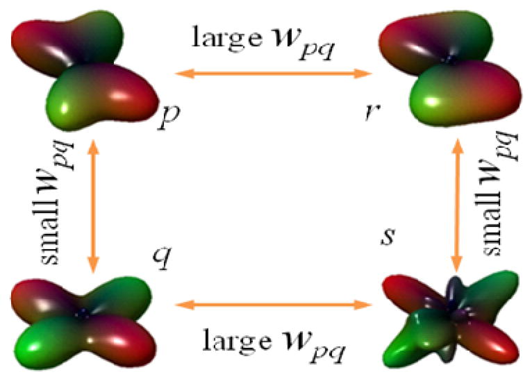
Schematic of properties of the spatial weight function. When neighboring ODFs are similar in shape, they should have a

MATERIALS AND METHODS

Simulation Studies

A software suite capable of simulating random 3D or user-generated 2D fiber configurations was developed, tested and exercised under a variety of imaging conditions. To investigate the accuracy of the proposed technique and compare it with conventional shQBI reconstruction without spatial constraints, we performed Monte Carlo simulations similar to those previously reported (Jones, 2004; Hess et al., 2006). Multiple fiber populations (varying from 2 to 100 fibers) distributed in 3D within a 20 × 20 × 20 voxel volume, in slow Gaussian exchange, with orientations separated by a prescribed angle, were modeled as the sum of prolate Gaussian functions with varying volume fractions and fractional anisotropies (FAs) of 0.75. The simulated MR signal was generated as the corresponding sum of multiple exponential decays. Non-zero volume fraction of water (with spherical ODF, FA of 0) was also added in order to realistically model fiber populations in the brain. A feature of our simulation software is that it allows the user to draw any number of linear fibers within the above 3D space, with user-selected FA and fiber width. This is particularly useful for modeling the effect of the spatial distribution of fibers on the ODF reconstruction, and to visualize possible performance improvements using spatial priors.

For the fiber population within each voxel, samples of the corresponding synthetic diffusion signal were obtained along non-collinear diffusion gradient orientations derived from the electrostatic repulsion algorithm (Jones 2004) and used to reconstruct the ODF. Complex-valued independent Gaussian noise was added to each sample in order to evaluate the dependence of the reconstruction on SNR, and the magnitude of the resulting data was used to calculate the ODF. SNR was defined as the ratio of the maximum signal intensity with no diffusion weighting to the standard deviation (SD) of the noise, corresponding to the SNR of the b = 0 s · mm⁻² images that were obtained experimentally. SNR values for the b = 0 s · mm⁻² non-DW data range from 1/10 to 10. This SNR range for the simulations was chosen to overlap the typical SNR range of the experimental HARDI data both in our experience and previously reported by other authors.

Large-scale Monte Carlo simulations were executed to evaluate the performance of the proposed spatial HARDI technique against the existing algorithm described in Hess et al., (2006) – “shQBI”, and its regularized version. Regularization in the latter case was performed using the Laplace-Beltrami operator described in (Sakaie et al., 2006; Descoteaux et al. 2007). Tikhonov regularization was also tested but was found to produce results either comparable to or worse than Laplace-Beltrami regularization, and was therefore dropped from further analysis. In addition, smoothed shQBI results were obtained by applying an isotropic smoothing operation with a 3×3×3 box filter as a post-processing step after standard shQBI reconstruction. The central element of the box filter is assigned a value of 5, and all other elements are assigned a value of 1. For each reconstructed ODF direction, the corresponding 3D volume was convolved with this box filter, giving a spatially smoothed version of the ODFs. This last method was implemented in order to address the important question of whether similar results to our proposed method can be obtained by simply smoothing the shQBI output.

All three reconstructions were evaluated with respect to various metrics including root mean square error (RMSE) of the ODF, error of generalized fractional anisotropy (GFA) (Hess et al., 2006; Tuch et al., 2004), fiber orientation accuracy, and smallest crossing fiber angle resolvable. These performance measures are well-known from previous reports, except orientation accuracy and angular resolution. The computation of the latter two is now briefly described.

Angular resolution refers to the smallest angle at which crossing fibers are resolvable by a given technique (Hess et al., 2006). Unfortunately it is difficult to automate the decision-making involved in resolving crossing fibers in the presence of significant noise and/or smoothing – this is usually done visually by an experienced user. Ultimately, the ability to resolve crossing fibers can be evaluated by the performance of subsequent fiber tractography steps. However, this does not provide an intrinsic angular resolution measure, being dependent on the properties of a separate tractography algorithm

To assess angular resolution, we implemented an unsupervised fiber detection module in lieu of tractography. This module infers the number of fibers present in a given voxel by detecting regional peaks in the 2D (azimuth and elevation) plot of ODF after Gaussian smoothing, in a manner similar to what has been described in other reports, e.g. (Tristan-Vega et al., 2009; Descoteaux et al., 2007). In order to reduce sensitivity to spurious peaks introduced by noise, the traditional approach was made more robust as described below. Significant peaks were defined as peaks with a minimum area of 10 degrees (azimuth) × 10 degrees (elevation) in the 2D plane, and minimum height of at least 40% of maximum peak height. A morphological erosion operation was also performed in order to remove irregularly-shaped (and hence erroneous) peaks. This fiber detection module was tested thoroughly, and its output was used to measure angular resolution, as follows. Two crossing fibers were deemed resolvable if the mean error in detecting the correct number of fibers, over a large number of repeated trials, was found to be less than 10%. There exist more advanced Bayesian fiber detection techniques (Hosey et al., 2005) which might improve on our basic detection module, but the time and complexity involved in implementing such a technique was not justified in the scope of this work.

Orientation accuracy was evaluated by taking single-fiber voxel populations and measuring the direction of the peak closest to the true fiber orientation. The angular difference between these two directions was defined as orientation accuracy. The closest peak was detected by starting at the given true peak orientation, and applying a brute force search within a specified neighborhood (22 degrees in elevation and azimuth) for the location of the maximum ODF. The maximum location is then iteratively refined by searching over successively smaller neighborhoods around the detected peak.

We note that the number of crossing fibers in our simulations can be two or more. RMSE and GFA-RMS are evaluated in every voxel whether having mixed fiber population or not. Orientation accuracy was evaluated in single fiber voxels only in order to preclude the effect of other fibers from contaminating the orientation accuracy value of the main fiber. Angular resolution was calculated at voxels with two fiber populations oriented at various angles. Three or more fiber voxels were precluded from this calculation because it is difficult to interpret the effect of the third fiber on the angular resolution between the first two fibers. Even if we could, the result would not necessarily increase our understanding of the proposed method.

Performance of the 3 or 4 competing algorithms (unregularized and/or regularized shQBI, smoothed shQBI and spatial HARDI) was evaluated using four criteria: root mean square error (RMSE) of the ODF, root mean square of the generalized fractional anisotropy (RMS-GFA), orientation accuracy and angular resolution.

In order to evaluate the sensitivity of all three or four methods to parameter choice, it may not be sufficient to evaluate these methods at fixed parameter settings, because the relative performance of different methods varies with parameter choice. An alternate way is now presented to capture these parameter-dependent performance differences and to evaluate each method over a wide range of parameter choice, through a joint investigation of two performance measures simultaneously with changing parameter choice. We believe this to be an important feature, because no single performance measure, whether RMSE, orientation accuracy or angular resolution, is by itself an adequate measure of overall performance of the method. Correct reconstruction of ODF, measured by RMSE, is probably more important for quantitative diffusion measurements, whereas angular resolution and orientation accuracy might be more relevant for subsequent tractography. In addition, these measures are somewhat conflicting in nature, meaning that it is sometimes possible to improve one at the cost of the other. For example, increasing regularization using any method can easily improve the orientation accuracy of a single-fiber ODF, but at the cost of higher RMSE. Unless parameter optimization was performed very carefully for each algorithm separately, it is difficult to state categorically how the competing methods compare. Therefore, the value of a method must necessarily depend on its performance jointly on a number of measures.

We plotted RMSE and orientation accuracy for each method as a curve parameterized by the algorithmic parameter under consideration – in this case the regularization factor. Algorithmic parameters specific to spatial HARDI (μ) was fixed at 0.1, and the regularization parameter λ was varied over the range [0.05, 0.3] in 12 increments for all three methods. Two SNR levels were used, and were plotted separately. In some ways this analysis technique is similar to the so-called L-curve analysis (Lin et al., 2004) which is useful in ascertaining optimal parameter choice, especially the regularization parameter.

In Vivo Experimental Studies

Whole-brain HARDI was performed on two adult male volunteers (23–34 years old) using a 3T Signa EXCITE scanner (GE Healthcare, Waukesha, WI) equipped with an eight-channel phased-array head coil. The imaging protocol was approved by the institutional review board at our medical center, and written informed consent was obtained from the participants. On one subject, a multislice single-shot echo-planar spin-echo pulse sequence was employed to obtain measurements at a diffusion weighting of b = 3000 s · mm⁻², where the diffusion-encoding directions were distributed uniformly over the surface of a sphere using electrostatic repulsion (Jones, 2004). Conventional Stejskal-Tanner diffusion encoding was applied with δ = 31.8 ms, Δ = 37.1 ms and g_rnax= 40 mT.m⁻¹, yielding a q-space radius of 534.7 cm⁻¹. An additional acquisition without diffusion weighting at b = 0 s · mm⁻² was also obtained. The total scan time for whole-brain acquisition of 131 diffusion-encoding directions was 39.6 min with TR/TE = 18 s/84 ms, NEX = 1, and isotropic 2-mm voxel resolution (FOV = 260 × 260 mm, matrix = 128 × 128, 68 interleaved slices with 2-mm slice thickness and no gap). On another subject, whole-brain HARDI was performed at 2.2-mm isotropic spatial resolution (FOV = 280 × 280 mm, matrix = 128 × 128, 60 interleaved slices with 2.2 mm slice thickness and no gap) using 55 diffusion encoding directions with TR/TE = 16.4 s/82 ms, for a total scan time of 15.3 min. Axial slices in both cases were oriented along the plane passing through the anterior and posterior commissures. Parallel acquisition of the DW data using the eight-channel transmit-receive EXCITE head coil was accomplished using the array spatial sensitivity encoding technique (GE Healthcare, Waukesha, WI, USA) with an acceleration factor of 2.

Reconstruction using all three methods was performed on these in vivo HARDI data sets. Reconstruction parameters were identical to the optimal parameters found during simulation studies: Regularization parameter and spatial prior weights were both set at 0.2. Spherical harmonics up to order four and order six were estimated.

Reconstruction and Visualization

For all three methods, ODF values were computed at locations corresponding to the vertices of a fourfold tessellated icosahedron, giving 642 directions. For ease of visualization of the results, ODFs were min-max normalized and plotted as a 3D surface. Points on the surface of the ODF were color-coded by direction according to the standard red (left–right), blue (superoinferior), and green (anteroposterior) convention used to represent the direction of the principal eigenvector in DTI. The ODF surfaces are overlaid onto a grayscale background corresponding to the generalized fractional anisotropy (GFA) within each voxel for visualization of the human subject data (Hagmann et al., 2007). The more anisotropic ODFs thus appear superimposed on brighter backgrounds, and the background appears dark in voxels with low GFA. All q-ball computations were performed using custom software written in MATLAB version 7.6 (MathWorks, Natick, MA, USA).

RESULTS

Units

RMSE and RMS-GFA are shown in arbitrary units, given by the error norm between (normalized) true and reconstructed ODFs – smaller is better. Orientation accuracy and angular resolution are in degrees – smaller is better.

Simulation studies

Performance of the 3 competing algorithms (Laplace-Beltrami regularized shQBI, smoothed shQBI and spatial HARDI) was evaluated. As the results in Figures 3 and 4 show, for harmonic order 4, neither the original spherical harmonic method nor post-processing by applying a directional smoothing filter is able to achieve the level of performance of the proposed spatially-constrained technique. A slight worsening of orientation accuracy and angular resolution is seen in spatial HARDI compared to smoothed shQBI; this points to our approach sacrificing modest amounts of angular resolution for significant gains in noise performance. The ODF peaks from all algorithms appear slightly misaligned with the fibers. We believe this to result from the (parsimonious) spherical harmonic basis, which is not rotation-invariant, and therefore does not guarantee perfect alignment.

Figure 3.

Simulated ODFs with crossing fibers, at SNR of 1.0, and harmonic order 4. Note the distortion caused in shQBI due to noise. Spatial HARDI exhibits sharper profiles compared to others, and is able to recover the crossing fiber profile in the center. Voxels with no fibers are not shown.

Figure 4.

Performance versus SNR, harmonic order 4, λ = 0.2, μ = 0.2. RMSE captures the overall mismatch between actual and noisy ODFs, GFA captures the mismatch in generalized fractional anisotropy, and orientation accuracy captures the mean mismatch in the estimated angle of the fibers.

In order to evaluate sensitivity of all three methods to parameter choice, Figure 5 shows RMSE and orientation accuracy versus SNR for two different parameter settings. Harmonic order was chosen as 6 for both. Relative performance of the three methods varies with parameter choice. Note the difference in performance from Figure 4, which is for a different model order and whose parameters were selected very carefully after an exhaustive search. This example serves to illustrate the difficulty in ascertaining performance of ODF reconstruction algorithms at user-selected, fixed values of algorithmic parameters.

Figure 5.

RMSE and orientation accuracy versus SNR for two different parameter settings. Harmonic order was chosen as 6 for both. (a) λ = 0.1, μ = 0.05 and (b) (a) λ = 0.05, μ = 0.25. Both (a) and (b) are special cases of curves similar to those shown in Figure 4.

Results of joint analysis of two performance measures with harmonic order 6, RMSE and orientation accuracy, are shown in Figure 6. The figure indicates that over a large range of regularization parameter, spatial HARDI is better at minimizing both RMS error and orientation error than the other two methods. Clearly, shQBI and its smoothed version both exceed the performance of spatial HARDI occasionally on a single performance measure, but not on both measures simultaneously. We chose RMSE and orientation accuracy in this investigation because of the known conflicting nature of these two measures. Unfortunately, this approach is not easily extendable to more than two measures simultaneously. RMS of GFA and angular resolution were not investigated in this work, but we expect similar results to Figure 6.

Figure 6.

Joint performance curves of reconstruction methods for various SNR levels. In each case the regularization parameter λ was varied in the range [0.05, 0.3] in 12 increments. Spatial HARDI reconstruction was performed at μ equal to λ in order to reduce possible degrees of freedom. The first three plots are shown on the same axes, and the last one on a different one for ease of viewing.

Execution time

As per Table 1, Spatial HARDI takes about 3–5× more time than sqQBI with smoothing. However, these numbers do not reflect the overhead associated with file input/output and preprocessing, which are shared by all algorithms but vary with image size and resolution. In realistic in vivo imaging situations we have found about 2× increase in overall execution time of spatialHARDI compared to sqQBI+smoothing.

Table 1.

Execution time (ms) of ODF reconstruction algorithms implemented in MATLAB v7.8.0

Harmonic Order	shQBI	shQBI+smoothing	spatialHARDI
4	0.13	0.49	1.7
6	0.09	0.42	2.3

In vivo studies

Figure 7 shows the three reconstructions for a region of interest (ROI) where fibers within the optic radiation, oriented in the anterior-posterior direction, co-exist with cortical fibers of the posterior temporal lobe, oriented left-right as shown in figure 7(a-b). Spherical harmonics up to order four were used, which were reconstructed from raw diffusion data in 36 directions and b-value of 3000. Figure 7(c) is the standard shQBI reconstruction with no regularization. Part (d) shows shQBI at regularization factor of 0.2, and (e) shows the result of a post-processing step involving spatial smoothing of (c). This was done in order to assess the utility of spatial smoothing as a post-reconstruction step with respect to both shQBI and spatial HARDI, which is shown in (f). Note that post-reconstruction spatial smoothing gives different ODF shapes than spatially constrained Bayesian reconstruction. Clearly spatial smoothing did not result in appreciable improvement over shQBI or regularized shQBI; consequently it has been dropped from subsequent examples.

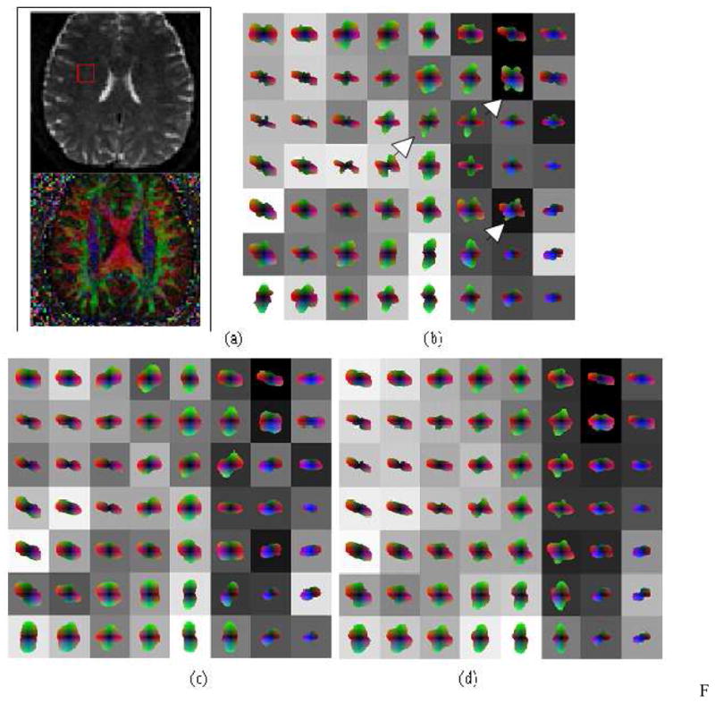
Figure 7.

Reconstruction of in vivo MR HARDI data, b=3000, 36 directions, order-4 harmonics: (a) T2 weighted MRI slice depicting region of interest, (b) corresponding color FA map, (c) shQBI, (d) regularized shQBI, (e) shQBI with post-reconstruction smoothing, and (f) spatial HARDI. Noteworthy ODFs are denoted by arrowheads.

It is interesting that the same diffusion data can produce sharp differences in reconstruction under various assumptions. The shQBI reconstructions all appear to show an abrupt boundary between the two fiber populations at the interface between second and third columns in Fig. 7. Note especially the voxels denoted by the white arrowhead in Fig. 7(f). In shQBI recons (c-e), these ODFs do not seem to give contiguous fiber bundles. It appears to us unlikely that neighboring voxels could have such divergent orientations without other voxels in the same neighborhood showing signs of mixed fiber populations due to partial volume averaging. The last row of shQBI shows incoherently oriented ODFs, particularly the fourth and fifth voxels imply existence of an A-P oriented fiber, but this is not supported by any of their neighbors. Spatial HARDI in contrast produces a jointly consistent but different configuration. Although the true configuration is difficult to determine in this case, at this level of prior weight (0.2), it is quite unlikely that spatial HARDI would have artifactually introduced a fiber configuration, unless there was support for it in the observed data itself. Note also that neighboring support comes not just from the slice shown but also its adjacent slices which are not shown. Fig. 7(f) depicts a mixed population of fibers in column 3, with medial-lateral fibers (in red) fanning out in the Anterior-Posterior (A-P, green) and Superior-Inferior (S-I, blue) directions. Finally, as shown in the center voxel (3^rd row and 3rd column) of Fig. 7(f), spatial HARDI managed to capture some ML-oriented fibers en route to/from the cortex within the A-P fibers -- these are definitely present anatomically but not depicted by any of the other methods.

Figure 8 shows the three reconstructions for an ROI in the anterior limb of the internal capsule, which is a well-known region of mainly cortico-thalamic fibers oriented in the anterior-posterior direction, along with some other fibers of mixed orientation. This region is shown by the red rectangle drawn in (a) and (b), which contain the T2-weighted image slice and the color FA maps respectively. Figs. (c-e) were reconstructed from a maximum spherical harmonic order of 4, and Figs. (f-h) from maximum order 6. In the 4-harmonic case, both shQBI and spatial HARDI reconstructions are able to resolve ODFs originating from the main A-P fiber population quire well. At this level of noise, an order-4 harmonic fit is sufficient to get good results in all cases. Imposition of spatial prior in (e) did not lead to any degradation of ODF profiles in the region denoted by the red rectangle in (e). This demonstrates that our method does not indiscriminately blur ODFs across neighboring voxels. Row 3 (f-h) show that a higher harmonic order of 6 caused overfitting of the data, leading to noise in the reconstructed shQBI. At a higher regularization factor, this noise was removed, but at the cost of appreciable blurring. The spatial HARDI reconstruction (h) overcomes the noise problem without leading to ODF blurring. For instance, compare the voxels indicated by the arrowheads for all three reconstructions.

Figure 8.

Reconstruction of in vivo MR HARDI data in the anterior limb of the internal capsule, b=3000, 36 directions: (a) T2 weighted MRI slice depicting region of interest, (b) corresponding FA map. Second row shows results with 4-order harmonics and third row shows results with 6-order harmonics. (c, f) shQBI, (d, g) regularized shQBI, (e, h) spatial HARDI. Note improved definition of the ODFs and better resolution of crossing fibers. Instances of crossing fiber resolution in spatial HARDI are denoted by yellow arrowheads in the right panel. Red box in (e) shows ODFs which are unaffected by differing inference in neighboring voxels.

Figure 9 shows the three reconstructions for a ROI in a region shown in (a) and (b) where Medial-Lateral (M-L, red, 3 left columns) oriented fibers to cortical areas coexist with A-P oriented fibers within the superior longitudinal fascicle (green, middle 3 columns) and S-I oriented projections of the corona radiata (blue, rightmost 2 columns). ODFs were reconstructed from order 6 spherical harmonics. These crossing fibers can be resolved in all reconstructions, but the main problem with shQBI in this case appears to be noise, which has led in some cases to spurious ODF peaks – some examples are indicated by arrowheads. Although regularization of shQBI succeeds in removing these spurious peaks, it does so at the cost of much poorer angular resolution, which might become an important limitation in this region of several coexisting fiber tracts. Imposition of the spatial prior in (d) removes spurious ODF peaks without degradation of ODF profiles, while at the same time faithfully resolving the extant crossing fiber configuration. Notice how easily each fiber population can be traced right through the ROI without encountering spurious ODF peaks, which might mislead a tractography algorithm, or ambiguity due to crossing fibers, which might cause computed tracks to end abruptly.

Figure 9.

Reconstruction of in vivo MR HARDI data, b=3000, 36 directions, 6-order harmonic reconstruction: (a) T2 MRI and FA map depicting region of interest, (b) shQBI, (c) regularized shQBI, (d) spatial HARDI. Note both noise reduction and improved coherence of fiber populations.

Figure 10 shows the effect of different numbers of gradient directions. We chose a ROI at the interface of M-L and S-I fibers within the right occipital white matter, shown in (a) and (b). This data was acquired at b=6000 and 131 directions and reconstructed with 6-order harmonics. A single voxel from the calcarine projections oriented in the diagonal direction was selected for detailed viewing; this voxel is adjacent to a fiber bundle oriented in the S-I direction. The original data, acquired at 131 directions, was subsampled to fewer directions (55, 33 and 25), as follows. The original data in (θ,φ) space was uniformly subsampled to the nearest regular tiling in (θ,φ) space; however this may or may not give the exact number we want, so from here we randomly throw away some directions until the desired number is reached. At the original 131 directions, all methods perform similarly. Due to decreasing SNR and lower angular resolution as the number of directions is decreased, shQBI reconstruction suffers from significant noise and spurious peaks, and is clearly unusable at 33 and 25 directions. Regularized shQBI is able to remove spurious peaks but at the cost of reduced angular resolution; finally it too fails at 25 directions because the dominant direction is simply incorrect. In clear contrast, spatial HARDI is able to maintain both orientation accuracy and angular resolution at all levels.

Figure 10.

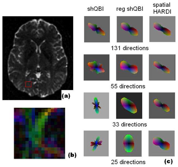
Reconstruction of in vivo data, b=6000, at various number of directions, 6-order harmonic reconstruction: (a) T2 MRI and (b) zoomed-in FA map depicting region of interest, (c) single voxel reconstruction with shQBI, regularized shQBI, and spatial HARDI. Our result maintains the orientation and angular resolution of the ODF in all cases.

DISCUSSION AND CONCLUSION

Although presented results pertain to the shQBI method, we note that it is easily applicable to any linear HARDI reconstruction technique. In addition to shQBI, other popular reconstruction methods that use radial basis functions – RBF-QBI (Tuch, 2004) and PASMRI (Jansons et al., 2003) - could have been used for this work. Spatial HARDI can also be used in conjunction with different regularization techniques, like Tikhonov regularization or the graduated Laplace-Beltrami regularization. Our approach can also be used within proposed model-based reconstructions like multi-tensor mixture models (Hosey et al., 2005; Tuch, 2002) or tensor distribution models (Jian et al., 2007). In all cases, we can write ODF reconstruction as a cost minimization problem similar to Eq. (1), where the use of spatial information adds an additional term to the minimization function.

Although not the focus of the present work, the proposed method can also be used to obtain conventional DTI reconstruction (“spatial DTI”), because diffusion tensors are estimated via a linear estimator, just like shQBI, PASMRI or RBF-QBI. Our experimentation with DTI reconstruction using spatial HARDI indicates performance similar to conventional DTI, with a small improvement in extremely noisy cases. This data is not shown in this paper, because our focus is on high angular resolution. For standard DTI reconstruction, there is really no need to acquire at high b-values and large number of directions. One potential use for spatial DTI would be to enable very high spatial resolution DTI by more faithfully reconstructing the tensor even at very low SNR.

The inclusion of spatially smoothed shQBI in our comparative results might appear unconventional – it is certainly not a standard technique reported anywhere that we are aware of – but we believe it serves an important purpose: it answers the question of whether spatial HARDI, which after all imposes spatial smoothness constraints, could be reproduced simply by spatially smoothing the conventional shQBI output. Presented results confirm that the two methods are very different, and that post-reconstruction smoothing is a suboptimal approach for imposing spatial smoothness constraints. Instead, spatial constraints should be imposed at the time of reconstruction, where it can usefully disambiguate noisy or incomplete observed data by supplying additional information. If one waits until after the reconstruction has completed, the noise or inadequate data quality have already propagated and cannot be easily removed at this stage. Our comparative results corroborate this fact, which is a well-known feature whenever Bayesian methods employing spatial priors were used for image estimation in various contexts – image segmentation (Zhang et al., 2001), parallel imaging reconstruction (Raj et al., 2007), etc.

Finally, our use of weighted norms via the neighborhood weights w_i,j has previously appeared in anatomically-constrained prior models for MR image reconstruction (e.g. Haldar et al., 2008 and references therein), where the weights are estimated from a set of prior reference images. In contrast we do not have access to appropriate reference images, since no other imaging modality exhibits directionally-variant diffusion-weighted tissue contrast. Consequently our optimization problem is harder, since the weights must also be jointly estimated along with the ODFs.

The proposed work serves as more robust and tolerant to measurement noise and time-limited acquisitions than current voxelwise methods of reconstructing ODFs. Our method can lead to more accurate and sensitive tractography outcomes, which in turn could lead to more precise and reliable surgical planning. Tractography is also being proposed as an input to advanced network-level analysis of brain neuronal connectivity (Hagmann et al., 2007). Again, the outcome of these tasks is crucially dependent on the accuracy and resolution, both spatial and angular, of reconstructed ODFs.

Limitations and Future Work

One limitation of the proposed method is its assumption of uncorrelated Gaussian noise. Although raw complex diffusion data does in fact have additive Gaussian noise, the same cannot be said for the observations e, which are obtained from the raw data in a highly non-linear fashion, especially with the use of parallel imaging. Many proposed noise models for HARDI are known (Kim et al., 2009; Jones et al., 2004), and it has been shown that the Gaussian assumption fails especially at very low signal levels. However, the Gaussian assumption in our method follows much of the literature, and has been shown to produce reasonable results. Of course, any given noise model can be incorporated in the formulation presented in Eqs. (1) – (4) by suitably altering the likelihood term; unfortunately the resulting cost minimization problem quickly becomes intractable in such cases. This is because the first term in Eq. (4) is no longer quadratic or even convex, characterized by multiple local minima that render optimization untenable. In this work our focus is to introduce spatial prior models rather than a detailed noise model. Our future work will involve extending our method to other noise models and obtaining efficient minimization algorithms to solve them.

Some very recent work (Canales-Rodríguez, et al., 2009; Barnett, A,. 2009) suggests that the q-ball model employed in our work, although widely used, might not be optimal or even a good approximation to Tuch’s original ODF model. Present work does not attempt to address this issue; however it should prove tractable to modify our approach to incorporate the latest approach advocated by Canales-Rodríguez, Barnett and co-workers. In any case, the present work is more concerned with how to exploit spatial constraints rather than with a specific q-ball model.

The prior penalty terms in Eq. (4) introduce some prior bias, which might be detrimental to accuracy. Fortunately, it is generally known in Bayesian literature (Raj et al., 2007; Lin et al., 2004) that a very small amount of bias can improve the conditioning of extremely badly-posed inverse problems. Still, there is always a trade-off between prior bias and conditioning of the problem, and the optimal point of this tradeoff must ultimately be determined by the user. For instance in Bayesian MR image reconstruction, too much regularization causes excessive smoothing and too little gives noise amplification due to poor matrix conditioning (Raj et al., 2007). Several techniques exist to evaluate this trade-off, including generalized cross validation (Golub et al., 1979) and L-curve analysis (Lin et al., 2004). In this paper we do not perform these analyses, because our experience has been that the result of such an analysis are specific to the experimental situation and cannot easily be transferred. Instead we chose a trial and error approach where the regularization parameters are varied in small increments within a feasible range, and the parameters that produce the best results (RMSE, angular resolution, etc) were chosen. This paper employs global, spatially invariant regularization parameters. Spatially varying parameters are in general much harder to validate due to a vastly greater parameter space, and there appears little justification in doing so since the essential local variability is already being captured in the weight matrix. The optimal parameters might change for different subjects and scans because they depend on SNR and image resolution. It might be possible that some sort of scaling law for λ and μ as a function of image resolution and SNR might accommodate inter-scan and inter-subject variability; these issues will form part of our future work. We also plan a visual evaluation by experts in neurology of whole brain tractography based on proposed ODFs.

The exact form of W(η) is an open question at this time, and most likely will depend on computational and tractability considerations. Since the weights should generally depend on the ODF configuration η, we denote an explicit dependence on η. This is a tricky issue from a statistical as well as computational standpoint, because it makes the minimization task non-linear and the cost function non-quadratic and/or non-convex. Here we have examined an interesting form of W(η), and proposed a simple iterative scheme whereby both W(η.) and η itself are updated alternately. Future work will look into the optimal choice of W(η).

Conclusion

In conclusion, we proposed a novel Bayesian approach to DTI and HARDI reconstruction, called Spatial HARDI, by exploiting the spatial coherence of the diffusion profiles of water molecules in vivo. Careful algorithm design enables the added Bayesian technology to be employed without impractical increase in overall execution time compared to standard shQBI reconstruction. Presented simulation and in vivo evidence suggests that Spatial HARDI can jointly improve RMSE and orientation accuracy of ODF reconstruction. Results from in vivo human brain data also indicates that the proposed method might be better at maintaining accurate ODFs for smaller numbers of acquisition directions (hence faster scans) compared to spatial smoothing or single-voxel ODF regularization.

Research Highlights.

• A New method to utilize spatial information to constrain the reconstruction of ODFs from raw diffusion MRI data

• Improves angular resolution and noise tolerance

• Spatial constraints in terms of a prior distributions, incorporated in a Bayesian formulation

• A Novel iterative algorithm based on LSQR

• Results indicate significant gains in angular resolution, crossing fibers and reconstruction SNR

• Possible impact: improved evaluation of white matter microstructural integrity in regions of crossing fibers and higher spatial/angular resolution.

References

- Alexander DC, Barker GJ, Arridge SR. Detection and modeling of non-Gaussian apparent diffusion coefficient profiles in human brain data. Magnetic Resonance in Medicine. 2002;48:331–340. doi: 10.1002/mrm.10209. [DOI] [PubMed] [Google Scholar]
- Anderson AW. Measurement of fiber orientation distributions using high angular resolution diffusion imaging. Magnetic Resonance in Medicine. 2005;54(5):1194–206. doi: 10.1002/mrm.20667. [DOI] [PubMed] [Google Scholar]
- Barnett A. Theory of Q-ball imaging redux: Implications for fiber tracking. Magnetic Resonance in Medicine. 2009;62(4):910–23. doi: 10.1002/mrm.22073. [DOI] [PubMed] [Google Scholar]
- Beaulieu C. The basis of anisotropic water diffusion in the nervous system—a technical review. MR Biomed. 2002;15:438–455. doi: 10.1002/nbm.782. [DOI] [PubMed] [Google Scholar]
- Campbell JS, Siddiqi K, Rymar VV, Sadikot AF, Pike GB. Flow-based fiber tracking with diffusion tensor and q-ball data: validation and comparison to principal diffusion direction techniques. NeuroImage. 2005;27:725–736. doi: 10.1016/j.neuroimage.2005.05.014. [DOI] [PubMed] [Google Scholar]
- Canales-Rodríguez EJ, Melie-García L, Iturria-Medina Y. Mathematical description of q-space in spherical coordinates: exact q-ball imaging. Magnetic Resonance in Medicine. 2009;61(6):1350–67. doi: 10.1002/mrm.21917. [DOI] [PubMed] [Google Scholar]
- Descoteaux M, Angelino E, Fitzgibbons S, Deriche R. Regularized, Fast, and Robust Analytical Q-Ball Imaging. Magnetic Resonance in Medicine. 2007;58:497–510. doi: 10.1002/mrm.21277. [DOI] [PubMed] [Google Scholar]
- Descoteaux M, Wiest-Daesslé N, Prima S, Barillot C, Deriche R. Impact of Rician adapted Non-Local Means filtering on HARDI. International Conference on Medical Image Computing and Computer-Assisted Intervention. 2008;11(2):122–130. doi: 10.1007/978-3-540-85990-1_15. [DOI] [PubMed] [Google Scholar]
- Frank LR. Characterization of anisotropy in high angular resolution diffusion weighted MRI. Magnetic Resonance in Medicine. 2002;47:1083–1099. doi: 10.1002/mrm.10156. [DOI] [PubMed] [Google Scholar]
- Gerchberg RW, Saxton WO. Practical algorithm for the determination of phase from image and diffraction plane pictures. Optik. 1972;35(2):237–250. [Google Scholar]
- Golub GH, Heath M, Wahba G. Generalized cross-validation as a method for choosing a good ridge parameter. Technometrics 1979 [Google Scholar]
- Goh A, Lenglet C, Thompson PM, Vidal R. A Nonparametric Riemannian Framework for Processing High Angular Resolution Diffusion Images (HARDI). Proceedings of Computer Vision and Pattern Recognition Conference; 2009.2009. [Google Scholar]
- Groemer H. Geometric applications of Fourier series and spherical harmonics. Cambridge University Press; 1996. [Google Scholar]
- Hagmann P, Kurant M, Gigandet X, Thiran P, Wedeen VJ, Meuli R, Thiran JP. Mapping human whole-brain structural networks with diffusion MRI. PLoS ONE. 2007;2(7):597. doi: 10.1371/journal.pone.0000597. [DOI] [PMC free article] [PubMed] [Google Scholar]
- Haldar JP, Hernando D, Song SK, Liang ZP. Anatomically constrained reconstruction from noisy data. Magnetic Resonance in Medicine. 2008;59(4):810–818. doi: 10.1002/mrm.21536. [DOI] [PubMed] [Google Scholar]
- Hess CP, Mukherjee P, Han ET, Xu D, Vigneron DB. Q-ball reconstruction of multimodal fiber orientations using the spherical harmonic basis. Magnetic Resonance in Medicine. 2006;56:104–117. doi: 10.1002/mrm.20931. [DOI] [PubMed] [Google Scholar]
- Hosey T, Williams G, Ansorge R. Inference of Multiple Fiber Orientations in High Angular Resolution Diffusion Imaging. Magnetic Resonance in Medicine. 2005;54:1480–1489. doi: 10.1002/mrm.20723. [DOI] [PubMed] [Google Scholar]
- Jansons KM, Alexander DC. Persistent angular structure: new insights from diffusion magnetic resonance imaging data. Inverse Problems. 2003;19:1031–1046. [Google Scholar]
- Jian B, Vemuri BC, özarslan E, Carney PR, Mareci TH. A novel tensor distribution model for the diffusion-weighted MR signal. NeuroImage. 2007;37(1):164–176. doi: 10.1016/j.neuroimage.2007.03.074. [DOI] [PMC free article] [PubMed] [Google Scholar]
- Jones DK. The effect of gradient sampling schemes on measures derived from diffusion tensor MRI: a Monte Carlo study. Magnetic Resonance in Medicine. 2004;51:807–815. doi: 10.1002/mrm.20033. [DOI] [PubMed] [Google Scholar]
- Kim Y, Thompson PM, Toga AW, Vese L, Zhan L. HARDI Denoising: Variational Regularization of the Spherical Apparent Diffusion Coefficient sADC. IPMI; 2009. [DOI] [PubMed] [Google Scholar]
- Lin F, Kwang K, Belliveau J, Wald L. Parallel imaging reconstruction using automatic regularization. Magnetic Resonance in Medicine. 2004;51:559–567. doi: 10.1002/mrm.10718. [DOI] [PubMed] [Google Scholar]
- Liu C, Bammer R, Acar B, Moseley ME. Characterizing non-Gaussian diffusion by using generalized diffusion tensors. Magnetic Resonance in Medicine. 2004;51:924–937. doi: 10.1002/mrm.20071. [DOI] [PubMed] [Google Scholar]
- Mori S, Crain BJ, Chacko VP, Van Zijl PM. Three-dimensional tracking of axonal projections in the brain by magnetic resonance imaging. Ann Neurol. 1999;45:265–269. doi: 10.1002/1531-8249(199902)45:2<265::aid-ana21>3.0.co;2-3. [DOI] [PubMed] [Google Scholar]
- Mukherjee P, Hess CP, Xu D, Han ET, Kelley DA, Vigneron DB. Development and initial evaluation of 7-T q-ball imaging of the human brain. Magn Reson Imaging. 2007 doi: 10.1016/j.mri. [DOI] [PMC free article] [PubMed] [Google Scholar]
- Ozarslan E, Mareci TH. Generalized diffusion tensor imaging and analytical relationships between diffusion tensor imaging and high angular resolution diffusion imaging. Magnetic Resonance in Medicine. 2003;50:955–965. doi: 10.1002/mrm.10596. [DOI] [PubMed] [Google Scholar]
- Ozarslan E, Shepherd TM, Vemuri BC, Blackband SJ, Mareci TH. Resolution of complex tissue microarchitecture using the diffusion orientation transform (DOT) Neuroimage. 2006;31(3):1086–103. doi: 10.1016/j.neuroimage.2006.01.024. [DOI] [PubMed] [Google Scholar]
- Paige CC, Saunders MA. LSQR: An Algorithm for Sparse Linear Equations And Sparse Least Squares. ACM Trans Math Soft. 1982;8:43–71. [Google Scholar]
- Perrin M, Poupon C, Rieul B, Leroux P, Constantinesco A, Mangin JF, Lebihan D. Validation of q-ball imaging with a diffusion fibre-crossing phantom on a clinical scanner. Phil Trans R Soc Lond B Biol Sci. 2005;360:881–891. doi: 10.1098/rstb.2005.1650. [DOI] [PMC free article] [PubMed] [Google Scholar]
- Press W, Teukolsky S, Vetterling W, Flannery B. Numerical recipes in C. 2. Cambridge University Press; 1992. [Google Scholar]
- Pruessmann KP, Weiger M, Scheidegger MB, Boesiger P. SENSE: sensitivity encoding for fast MRI. Magnetic Resonance in Medicine. 1999;42:952–962. [PubMed] [Google Scholar]
- Raj A, Singh G, Zabih R, Kressler B, Wang Y, Schuff N, Weiner M. Bayesian Parallel Imaging with Edge-Preserving Priors. Magnetic Resonance in Medicine. 2007;57(1):8–21. doi: 10.1002/mrm.21012. [DOI] [PMC free article] [PubMed] [Google Scholar]
- Sakaie KE, Lowe MJ. An objective method for regularization of fiber orientation distributions derived from diffusion-weighted MRI. NeuroImage. 2006 doi: 10.1016/j.neuroimage.2006.08.034. [DOI] [PubMed] [Google Scholar]
- Tournier JD, Calamante F, Gadian DG, Connelly A. Direct estimation of the fiber orientation density function from diffusion-weighted MRI data using spherical deconvolution. Neuroimage. 2004;23:1176–1185. doi: 10.1016/j.neuroimage.2004.07.037. [DOI] [PubMed] [Google Scholar]
- Tristán-Vega A, Westin CF, Aja-Fernández S. Estimation of fiber Orientation Probability Density Functions in High Angular Resolution Diffusion Imaging. NeuroImage. 2009;47:638–650. doi: 10.1016/j.neuroimage.2009.04.049. [DOI] [PubMed] [Google Scholar]
- Tuch DS. Q-ball imaging. Magnetic Resonance in Medicine. 2004;52:1358–72. doi: 10.1002/mrm.20279. [DOI] [PubMed] [Google Scholar]
- Tuch DS. Q-ball imaging of macaque white matter architecture. Phil Trans R Soc B Biol Sci. 2005;360:869–879. doi: 10.1098/rstb.2005.1651. [DOI] [PMC free article] [PubMed] [Google Scholar]
- Tuch DS, Reese TG, Wiegell MR, Makris N, Belliveau JW, Wedeen VJ. High angular resolution diffusion imaging reveals intravoxel white matter fiber heterogeneity. Magnetic Resonance in Medicine. 2002;48:577–82. doi: 10.1002/mrm.10268. [DOI] [PubMed] [Google Scholar]
- Zhan W, Stein EA, Yang Y. Mapping the orientation of intravoxel crossing fibers based on the phase information of diffusion circular spectrum. Neuroimage. 2004;23:1358–1369. doi: 10.1016/j.neuroimage.2004.07.062. [DOI] [PubMed] [Google Scholar]
- Zhang Y, Brady M, Smith S. Segmentation of Brain MR Images through hidden markov random field model and the expectation maximization algorithm. IEEE Transactions on Medical Imaging. 2001;20:45–57. doi: 10.1109/42.906424. [DOI] [PubMed] [Google Scholar]