Bayesian On-line Learning of the Hazard Rate in Change-Point Problems

Abstract

Change-point models are generative models of time-varying data in which the underlying generative parameters undergo discontinuous changes at different points in time known as change-points. Change-points often represent important events in the underlying processes, like a change in brain state reflected in EEG data or a change in the value of a company reflected in its stock price. However, change-points can be difficult to identify in noisy data streams. Previous attempts to identify change-points on-line using Bayesian inference relied on specifying in advance the rate at which they occur, called the hazard rate (h). This approach leads to predictions that can depend strongly on the choice of h and is unable to deal optimally with systems in which h is not constant in time. In this paper we overcome these limitations by developing a hierarchical extension to earlier models. This approach allows h itself to be inferred from the data, which in turn helps to identify when change-points occur. We show that our approach can effectively identify change-points in both toy and real data sets with complex hazard rates and how it can be used as an ideal-observer model for human and animal behavior when faced with rapidly changing inputs.

1 Introduction

Whether one is a rat in a lab or a banker on Wall Street, making good, on-line inferences about the present to help predict the future is important for survival. However, such inferences can be difficult in a noisy and dynamic environment. In this paper we consider the problem of Bayesian on-line inference in models of dynamic environments that are characterized by “change-points,” which are defined as abrupt and potentially unsignaled events that have the effect of separating the observed time-series into independent epochs.

Such change-point models have been developed and applied to a variety of data, including stock markets (Chen and Gupta, 1997; Xuan and Murphy, 2007; Koop and Potter, 2004; Hsu, 1977), process control (Aroian and Levene, 1950), disease demographics (Denison and Holmes, 2001), DNA (Liu and Lawrence, 1999; Fearnhead and Liu, 2007), EEG (Bodenstein and Praetorius, 1977; Barlow et al., 1981), NMR (Adams and MacKay, 2007; Fearnhead, 2006), and the bee “waggle dance” (Xuan and Murphy, 2007). However, most of this progress has been restricted to offline inference, which uses the entire data stream (past, present, and future) to infer change-point locations (Smith, 1975; Barry and Hartigan, 1993; Stephens, 1994; Green, 1995; Chib, 1998; Fearnhead, 2006). Existing on-line approaches also have practical limitations, in particular requiring the unrealistic assumption that the frequency with which change-points occur, known as the hazard rate, h, is fixed and known in advance (Steyvers and Brown, 2006; Fearnhead and Liu, 2007; Adams and MacKay, 2007).

In this paper we we remove this limitation and present a novel Bayesian algorithm that can make on-line inferences about change-points in data in which the hazard rate is unknown and can itself undergo unsignaled change-points. The paper is organized as follows. We first review the previous Bayesian models that form the basis of our approach, paying particular attention to the limitations implied by a pre-specified hazard rate (section 2). We then show how these models can be extended to achieve on-line inference of a constant hazard rate (section 3) and a piecewise constant hazard rate in a change-point hierarchy (section 4). We then address ways of making the computations tractable by node pruning (section 5), give some numerical examples to show the effectiveness of this approach (section 6), and conclude (section 7).

2 Inference when hazard rate is known

Here we briefly review previous models that provide exact and efficient means for optimal, on-line inference in change-point problems (Fearnhead and Liu, 2007; Adams and MacKay, 2007). These models are based on the observation that the ability to identify a change-point depends critically on knowledge of the generative process that was active before the change-point. Thus, these models keep track of “runs” of data generated under stable conditions. However, these models require the hazard rate to be specified in advance, which we show can strongly affect model output.

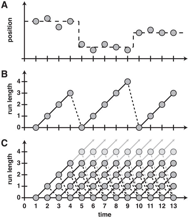
For example, consider the simple change-point process illustrated in figure 1A. The data points (filled circles) are generated by adding Gaussian random noise to a mean value (dashed line). The mean value varies in a piecewise constant manner over time, changing abruptly at change-points but otherwise staying constant. Thus, sample-by-sample fluctuations in the data can reflect both noise and change-points. To predict the position of the data point at time 14, the last four points should be used to compute the current average with the smallest effects of sample-by-sample noise. These points represent the run-length, r_t, which is defined as the number of time steps since the most recent change-point. Run-lengths are plotted for the current example in figure 1B. Note that r_t follows a relatively simple time course, either increasing by one on time steps between change-points or falling to zero at a change-point.

Figure 1.

Cartoon illustrating a simple change-point problem. A. Data points (circles) are generated by adding random noise to an underlying mean (dashed line) that undergoes two change-points, at times 5 and 10. B. The number of points since the last change-point, or run-length, is plotted as a function of time for the same example. The run-length increases by one when there is no change-point (black line) and decreases to zero when there is one (dashed black line). C Schematic of the message-passing updating rule from (Adams and MacKay, 2007). Starting from time 1, all of the weight is on the node at run-length 0. At time 2 this node then sends messages to nodes at run-lengths 1 and 0. From there each node sends two messages, one increasing the run-length by one and the other back to the node at r_t = 0. Using these input messages, each node updates its weight, p(r_t|x_1:t).

In general, the positions of change-points are not specified in advance but instead must be inferred from the data. Thus, optimal predictions of the next data point should consider all possible run-lengths and weigh them by the probability of the run-length given the data. More formally, if we write x_t as the data at time t and x_1:t for the set of data {x₁, x₂, …, x_t}, then the problem of prediction is equivalent to computing the predictive distribution, p (x_t+1|x_1:t). This distribution can be written in terms of the distribution of run-lengths given the previous data, p(r_t|x_1:t), as

$$p({\mathbf{x}}_{t+1}\mid {\mathbf{x}}_{1:t})=\sum _{r_t}p({\mathbf{x}}_{t+1}\mid {\mathbf{x}}_t^{(r_t)})p(r_t\mid {\mathbf{x}}_{1:t})$$ (1)

where ${\mathbf{x}}_t^{(r_t)}(={\mathbf{x}}_{t-r_t+1:t})$ is the set of most recent data corresponding to run-length r_t. The run-length distribution p(r_t|x_1:t) is computed recursively as

$$p(r_t\mid {\mathbf{x}}_{1:t})=\frac{p(r_t,{\mathbf{x}}_{1:t})}{p({\mathbf{x}}_{1:t})}$$ (2)

where

$$p({\mathbf{x}}_{1:t})=\sum _{r_t}p(r_t,{\mathbf{x}}_{1:t})$$ (3)

The recursion relation for p(r_t, x_1:t) can then be derived by writing it as the marginal of p(r_t, r_t−1, x_1:t) over r_t−1:

$$\begin{array}{l}p(r_t,{\mathbf{x}}_{1:t})=\sum _{r_{t-1}}p(r_t,r_{t-1},{\mathbf{x}}_{1:t})\\ =\sum _{r_{t-1}}p(r_t,{\mathbf{x}}_t\mid r_{t-1},{\mathbf{x}}_{1:t-1})p(r_{t-1},{\mathbf{x}}_{1:t-1})\\ =\sum _{r_{t-1}}p(r_t\mid r_{t-1})p({\mathbf{x}}_t\mid {\mathbf{x}}_{t-1}^{(r_{t-1})})p(r_{t-1},{\mathbf{x}}_{1:t-1})\end{array}$$ (4)

where $p({\mathbf{x}}_t\mid {\mathbf{x}}_{t-1}^{(r_{t-1})})$ is the predictive distribution given the most recent data points and p(r_t|r_t−1) is the change-point prior. This sum is made tractable because of the simple update rule for r_t, which can either increase by one or decrease to zero. Assuming that the prior probability of a change-point is given by the pre-specified hazard rate h (which for simplicity we assume to be independent of r_t), then:

$$p(r_t\mid r_{t-1})=\{\begin{array}{ll}1-h\hfill & \text{if}{r}_t=r_{t-1}+1\hfill \\ h\hfill & \text{if}{r}_t=0\hfill \\ 0\hfill & \text{otherwise}\hfill \end{array}$$ (5)

These equations lead to the “message-passing update rule” for p(r_t|x_1:t), depicted in figure 1C. In particular, each possible run-length r_t at time t corresponds to a node in the graph, (r_t, t), that can be thought of as an object made up of two components: a weight equal to p(r_t|x_1:t) and the predictive distribution over x_t+1 given the last r_t data points, $p({\mathbf{x}}_{t+1}\mid {\mathbf{x}}_t^{(r_t)})$. The algorithm updates by passing messages from all of the nodes at time t to their children at time t + 1, updating their individual weights and predictive distributions accordingly. Thanks to the change-point prior (equation 5), each node, (r_t, t), has only two children: a unique child, (r_t+1 = r_t+1, t+1), that corresponds to the run-length increasing by one, and a shared child, (r_t+1 = 0, t+1), that corresponds to the occurrence of a change-point. Thus the number of messages varies only linearly with the number of nodes. As noted in (Adams and MacKay, 2007), this approach is particularly suited to cases where the generative and prior distributions are members of the conjugate-exponential family, because in this case the predictive distributions $p({\mathbf{x}}_t\mid {\mathbf{x}}_{t-1}^{(r_{t-1})})$ can be fully described by a finite number of sufficient statistics (see supplementary material and (Wainwright and Jordan, 2008) for a more thorough introduction).

This message-passing approach can be thought of as the forward sweep of a forward-backward algorithm applied to a hidden Markov model (HMM) in which the states correspond to different values of the run-length. The HMM approach to change-point models was developed in (Chib, 1998), where the author used Monte Carlo methods to perform inference in a model with a pre-specified number of change-points. See (Paquet, 2007) for more details of the HMM interpretation of the Adams-MacKay algorithm.

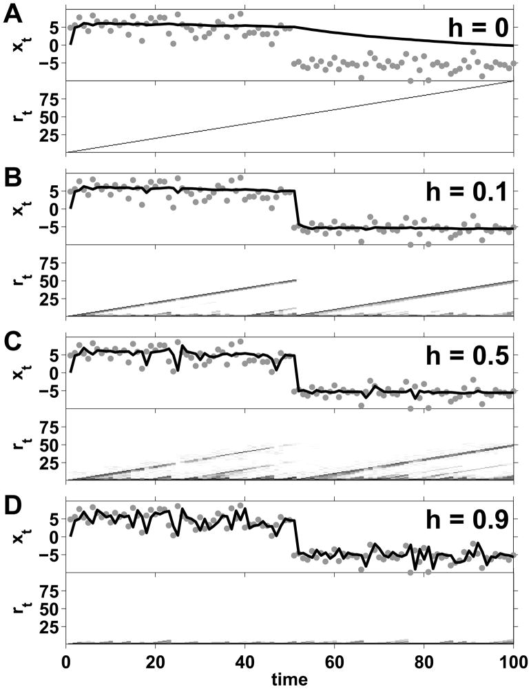
Despite excellent performance on many different data sets (Adams and MacKay, 2007; Fearnhead and Liu, 2007), a major limitation of this approach is that the hazard rate, h, must be specified in advance. Figure 2 highlights this limitation by plotting the output of the algorithm for the same data over time for different settings of h. Setting h to zero disallows the possibility of finding any change-points (figure 2A). In this case, the predictive mean at time t + 1 is just the mean of all the data points up to time t. The run-length distribution over time (bottom half of the panel) is zero everywhere except at r_t = t − 1, where it is one. Increasing h to 0.1 results in recognition of the change-point at t = 50 and seemingly appropriate estimates of the mean both before and after that point (figure 2B). Increasing h further still to 0.5 (figure 2C) and 0.9 (figure 2D) results in more and more change-points being identified and, as a result, more volatile estimates of the mean are produced that depend increasingly on the most recent data point.

Figure 2.

Effect of changing the hazard rate on the mean of the predictive distribution generated by the algorithm in (Adams and MacKay, 2007) for a single data set. Each panel shows a different setting of the hazard rate h, as indicated. The top half of each panel shows the data (gray dots) along with the model’s predicted mean in black. The bottom half of each panel shows the logarithm of the run-length distribution, log p(r_t|x_1:t), with darker shades corresponding to higher probabilities. Clearly the predictions are heavily influenced by the choice of h and, without knowing the actual change-point locations, it is not obvious to tell which one is better matched to the data.

Thus, the performance of models that require a pre-specified hazard rate can depend critically on which value is chosen, but which value is “best” is not always obvious in advance. Here we aim to remove this limitation by proposing a novel, hierarchical Bayesian approach for the on-line estimation of the hazard rate in change-point problems. This approach allows for optimal inference in more demanding problems in which the hazard rate is not given and can vary (in a piecewise constant manner) over time.

3 On-line inference of a constant hazard rate

In this section we develop a Bayesian model for inferring a constant hazard rate from raw data sequences. We model change-points as i.i.d. samples from a Bernoulli distribution, the rate of which is given by the unknown hazard rate. We develop our model by first considering the straightforward case in which change-point locations are known, then address the more challenging case in which change-point locations are unknown.

3.1 Known change-point positions

Suppose that the locations of change-points in a given sequence are known. Because change-points are all-or-nothing events, we can think of them as being generated (in discrete time) as samples from a Bernoulli process with a rate equal to the hazard rate. The hazard rate can then be inferred as the rate of the Bernoulli process given the binary observations.

Let y_t be a binary variable that denotes the presence (y_t = 1) or absence (y_t = 0) of a change-point at time t. Also define h̃_t+1 = p(y_t+1 = 1|y_1:t) as the inferred prediction of the hazard rate for time t + 1, which can be computed by writing p(y_t+1|y_1:t) as a marginal over the hazard rate:

$$\begin{array}{l}p(y_{t+1}\mid y_{1:t})={\int }_0^{1}p(y_{t+1}\mid h)p(h\mid y_{1:t})dh\\ =\frac{{\int }_0^{1}p(h){\prod }_{i=1}^{t+1}p(y_i\mid h)dh}{{\int }_0^{1}p(h){\prod }_{i=1}^{t}p(y_i\mid h)dh}\end{array}$$ (6)

where p(h) is the prior over the hazard rate.

By definition, p(y_i = 1|h) = h and p(y_i = 0|h) = 1 − h, and so assuming a Beta prior on h of the form

$$p(h\mid a_0,b_0)=\text{Beta}(h;a_0,b_0)=\frac{\mathrm{\Gamma }(a_0+b_0)}{\mathrm{\Gamma }(a_0)\mathrm{\Gamma }(b_0)}{h}^{a_0-1}{(1-h)}^{b_0-1}$$ (7)

gives

$$\begin{array}{l}p(y_{t+1}\mid y_{1:t})=\frac{{\int }_0^1{h}^{a_{t+1}+a_0-1}{(1-h)}^{b_{t+1}+b_0-1}dh}{{\int }_0^1{h}^{a_t}{(1-h)}^{b_t}dh}\\ =\frac{\mathrm{\Gamma }(a_{t+1}+a_0)\mathrm{\Gamma }(b_{t+1}+b_0)\mathrm{\Gamma }(a_t+b_t+a_0+b_0-1)}{\mathrm{\Gamma }(a_t+a_0)\mathrm{\Gamma }(b_t+b_0)\mathrm{\Gamma }(a_{t+1}+b_{t+1}+a_0+b_0-1)}\end{array}$$ (8)

where a_t is the number of change-points up to and including time t and b_t = t − a_t is the number of non-change-points up to time t. Γ(·) is the Gamma function.

Also by definition, a_t+1 = a_t + 1 if there is a change-point, otherwise a_t+1 = a_t, and thus

$$\begin{array}{l}p(y_{t+1}=1\mid y_{1:t})={\stackrel{\sim }{h}}_{t+1}=\frac{a_t+a_0}{a_t+b_t+a_0+b_0}\\ p(y_{t+1}=0\mid y_{1:t})=1-{\stackrel{\sim }{h}}_{t+1}=\frac{b_t+a_0}{a_t+b_t+a_0+b_0}\end{array}$$ (9)

Therefore, because b_t = t − a_t + b₀, if the positions of the change-points are known, predicting the hazard rate, h̃_t+1, requires keeping track of only the number of change-points, a_t, up to time, t. This advantage is a direct consequence of modeling the change-points as samples from a Bernoulli distribution with constant hazard rate, because a_t and b_t are the sufficient statistics of the predictive distribution.

3.2 Unknown change-point positions

When the locations of the change-points are unknown, we do not know the change-point count, a_t, with certainty and we must maintain a joint probability distribution over both a_t and r_t given the data, p(r_t, a_t|x_1:t). As in the case of constant h, this distribution can be computed recursively. In particular,

$$\begin{array}{l}p({\mathbf{x}}_{t+1}\mid {\mathbf{x}}_{1:t})=\sum _{r_t}\sum _{a_t}p({\mathbf{x}}_{t+1}\mid r_t,a_t,{\mathbf{x}}_{1:t})p(r_t,a_t\mid {\mathbf{x}}_{1:t})\\ =\sum _{r_t}\sum _{a_t}p({\mathbf{x}}_{t+1}\mid {\mathbf{x}}_t^{(r_t)})p(r_t,a_t\mid {\mathbf{x}}_{1:t})\end{array}$$ (10)

p(r_t, a_t|x_1:t) can be related to p(r_t, a_t, x_1:t) via

$$p(r_t,a_t\mid {\mathbf{x}}_{1:t})=\frac{p(r_t,a_t,{\mathbf{x}}_{1:t})}{{\sum }_{r_t}{\sum }_{a_t}p(r_t,a_t,{\mathbf{x}}_{1:t})}$$ (11)

and p(r_t, a_t, x_1:t) can be computed recursively

$$\begin{array}{l}p(r_t,a_t,{\mathbf{x}}_{1:t})=\sum _{r_{t-1}}\sum _{a_{t-1}}p(r_t,r_{t-1},a_t,a_{t-1},{\mathbf{x}}_{1:t})\\ =\sum _{r_{t-1}}\sum _{a_{t-1}}p(r_t,a_t,{\mathbf{x}}_t\mid r_{t-1},a_{t-1},{\mathbf{x}}_{1:t-1})p(r_{t-1},a_{t-1},{\mathbf{x}}_{1:t-1})\\ =\sum _{r_{t-1}}\sum _{a_{t-1}}p(r_t,a_t\mid r_{t-1},a_{t-1})p({\mathbf{x}}_t\mid {\mathbf{x}}_{t-1}^{(r_{t-1})})p(r_{t-1},a_{t-1},{\mathbf{x}}_{1:t-1})\end{array}$$ (12)

Furthermore, the explicit form of the change-point prior, p(r_t, a_t|r_t−1, a_t−1), can be written as a marginal over the hazard rate:

$$\begin{array}{l}p(r_t,a_t\mid r_{t-1},a_{t-1})={\int }_0^{1}p(r_t,a_t\mid h,r_{t-1},a_{t-1})p(h\mid r_{t-1},a_{t-1})dh\\ =\frac{\mathrm{\Gamma }(a_{t-1}+1)\mathrm{\Gamma }(b_{t-1}+1)}{\mathrm{\Gamma }(a_{t-1}+b_{t-1}+1)}{\int }_0^{1}p(r_t,a_t\mid h,r_{t-1},a_{t-1})h^{a_{t-1}}{(1-h)}^{b_{t-1}}dh\end{array}$$ (13)

with

$$p(r_t,a_t\mid h,r_{t-1},a_{t-1})=\{\begin{array}{ll}1-h\hfill & \text{if}{r}_t=r_{t-1}+1\text{and}{a}_t=a_{t-1}\hfill \\ h\hfill & \text{if}{r}_t=0\text{and}{a}_t=a_{t-1}+1\hfill \\ 0\hfill & \text{otherwise}\hfill \end{array}$$ (14)

where the last line of equation 13 and the form of equation 14 come directly from our assumption that change-points are generated as i.i.d. samples from a Bernoulli distribution.

Thus, performing the requisite integrals gives:

$$p(r_t,a_t\mid r_{t-1},a_{t-1})=\{\begin{array}{ll}\frac{b_{t-1}+1}{a_{t-1}+b_{t-1}+2}=1-{\stackrel{\sim }{h}}_t\hfill & \text{if}{r}_t=r_{t-1}+1\text{and}{a}_t=a_{t-1}\hfill \\ \frac{a_{t-1}+1}{a_{t-1}+b_{t-1}+2}={\stackrel{\sim }{h}}_t\hfill & \text{if}{r}_t=0\text{and}{a}_t=a_{t-1}+1\hfill \\ 0\hfill & \text{otherwise}\hfill \end{array}$$ (15)

Note the similarity between this and equation 5, where the only difference is that we are using the inferred hazard rate h̃_t instead of the pre-specified hazard rate h. Using this form for the change-point prior leads to a simple message-passing algorithm for the recursive update of p(r_t, a_t|x_1:t) that is very similar to the case in which h is constant (see supplementary material). The effectiveness of this approach for inferring a constant hazard rate from toy data is shown in figure 3.

Figure 3.

Inference of a constant hazard rate for a toy problem. A. The raw data (circles) and the predicted mean (solid line) plotted versus time. The actual change-point locations from the generative process are shown by the gray vertical lines. B. The marginal run-length distribution p(r_t|x_1:t) = Σ_at p(r_t, a_t|x_1:t) versus time. C. The marginal distribution over the number of change-points, p(a_t|x_1:t) = Σ_rt p(r_t, a_t|x_1:t), versus time. D. The maximum likelihood on-line estimate of the hazard rate (solid black line) quickly converges to the actual hazard rate (dashed black line).

4 Estimation of hazard rates in a change-point hierarchy

In this section we relax the constraint that the hazard rate is constant over time. Instead, we assume that the hazard rate is piecewise constant and is itself generated by a change-point process with its own, smaller hazard rate. More generally, we consider the possibility that this “second-order” hazard rate is generated from yet another change-point process with an even smaller, third-order hazard rate, and so on, to create what we term a “change-point hierarchy” of arbitrary depth. We describe first this generative model then how it is used for on-line inference.

4.1 The change-point hierarchy generative model

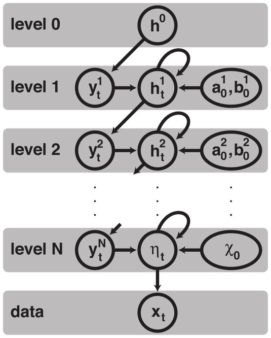
A schematic illustrating the general change-point hierarchy generative model is shown in figure 4. The inputs to the generative model are the top-level hazard rate, h⁽⁰⁾; the parameters for the priors on intermediate level hazard-rate distributions, ${\mathbf{a}}_0=\left\{a_0^{(1)},a_0^{(2)},\dots ,a_0^{(N)}\right\}$ and ${\mathbf{b}}_0=\left\{b_0^{(1)},b_0^{(2)},\dots ,b_0^{(N)}\right\}$; and the parameters, χ_p, that determine the prior distribution over the parameters, η, of the generative distribution. The initial values of the hazard rates, $h_{t=0}^{(n)}$, at all intermediate levels, n = 1 to N − 1, are sampled from beta distributions with parameters $a_0^{(n)}$ and $b_0^{(n)}$. The initial parameter values, η₀, for the generative distribution are sampled from the prior parameterized by χ_p.

Figure 4.

Illustration of the generative model corresponding to the change-point hierarchy. See text for details.

The generative process starts at level 0 and uses the top level hazard rate, h⁽⁰⁾, to sample the change-point locations for level 1. Specifically, for t = 1 to T_max, $y_t^{(1)}$ is sampled from a Bernoulli distribution with rate h⁽⁰⁾. If $y_t^{(1)}=1$ then there is a change-point at time t and $h_t^{(1)}$ is sampled from a beta distribution with parameters $a_0^{(1)}$ and $b_0^{(1)}$. If $y_{(t)}^{(1)}=0$ then there is no change-point and $h_t^{(1)}=h_{t-1}^{(1)}$.

Next, to get the change-point locations for level 2, $y_t^{(2)}$ is sampled from a Bernoulli process with rate $h_t^{(1)}$. As for level 1, if $y_t^{(2)}=1$ then there is a change-point and $h_t^{(2)}$ is sampled from a beta distribution with parameters $a_0^{(2)}$ and $b_0^{(2)}$. Otherwise, if $y_t^{(2)}=0$ there is no change-point and $h_t^{(2)}=h_{t-1}^{(2)}$.

This pattern is the continued down the hierarchy until level N is reached. At that point, instead of sampling a hazard rate, we sample the prior parameters of the generative distribution, η_t, from the prior parameterized by χ_p. Finally the data, x_t, are sampled from the data distribution parameterized by η_t.

Note that this model of a change-point hierarchy assumes that all of the hazard rates are independent of the time since the last change-point. This simplifying assumption is key to making the inference problem tractable but comes at the expense of excluding generative models with with hazard rates that can depend on the current run length.

4.2 On-line inference of hazard rate using a three-level hierarchy model

We now show how to infer hazard rates using the simplest example of a change-point hierarchy, with just three levels. We leave the general, N-level case to the supplementary material.

The approach here is similar to that of section 3, with two primary differences. The first is that we must now keep track of two kinds of run-length: the data-level run-length that we have already encountered, corresponding to the number of data points used to compute the predictive distribution of the data, $r_t^{(2)}$; and the high-level run-length, corresponding to the number of data points used in the computation of the hazard rate, $r_t^{(1)}$. The higher-order run-length can be written as

$$r_t^{(1)}=(a_t-a_0)+(b_t-b_0)$$ (16)

where a₀ and b₀ are the pre-defined prior parameters of the beta distribution on $h_t^{(1)}$, and a_t and b_t take on similar meanings as in section 3, with (a_t − a₀) the number of bottom-level change-points and (b_t − b₀) the number of non-change-points seen up to time t.

The second difference with section 3 is that, because we allow for change-points in level 1, $r_t^{(1)}$ can transition to zero. Thus, to compute the predictive distribution, we must maintain a probability distribution over $r_t^{(2)},r_t^{(1)}$, and a_t. Equivalently, because of equation 16, this distribution can be expressed over $r_t^{(2)}$, a_t, and b_t and we can drop the superscript on $r_t^{(2)}$ to refer, unambiguously, to the data-level run-length as r_t.

Thus, we can write the predictive distribution p(x_t+1|x_1:t) as

$$p({\mathbf{x}}_{t+1}\mid {\mathbf{x}}_{1:t})=\sum _{r_t}\sum _{a_t}\sum _{b_t}p({\mathbf{x}}_{t+1}\mid {\mathbf{x}}_t^{(r_t)})p(r_t,a_t,b_t\mid {\mathbf{x}}_{1:t})$$ (17)

where p(r_t, a_t, b_t|x_1:t) is given by

$$p(r_t,a_t,b_t\mid {\mathbf{x}}_{1:t})=\frac{p(r_t,a_t,b_t,{\mathbf{x}}_{1:t})}{{\sum }_{r_t}{\sum }_{a_t}{\sum }_{b_t}p(r_t,a_t,b_t,{\mathbf{x}}_{1:t})}$$ (18)

and p(r_t, a_t, b_t, x_1:t) can be computed recursively, because

$$\begin{array}{l}p(r_t,a_t,b_t,{\mathbf{x}}_{1:t})=\sum _{r_{t-1}}\sum _{a_{t-1}}\sum _{b_{t-1}}p(r_t,r_{t-1},a_t,a_{t-1},b_t,b_{t-1},{\mathbf{x}}_{1:t})\\ =\sum _{r_{t-1}}\sum _{a_{t-1}}\sum _{b_{t-1}}p(r_t,a_t,b_t,{\mathbf{x}}_t\mid r_{t-1},a_{t-1},b_{t-1},{\mathbf{x}}_{1:t-1})p(r_{t-1},a_{t-1},b_{t-1},{\mathbf{x}}_{1:t-1})\\ =\sum _{r_{t-1}}\sum _{a_{t-1}}\sum _{b_{t-1}}p(r_t,a_t,b_t\mid r_{t-1},a_{t-1},b_{t-1})p({\mathbf{x}}_t\mid {\mathbf{x}}_{t-1}^{(r_{t-1})})p(r_{t-1},a_{t-1},b_{t-1},{\mathbf{x}}_{1:t-1})\end{array}$$ (19)

The change-point prior, p(r_t, a_t, b_t|r_t−1, a_t−1, b_t−1) can be written as the marginal over the hazard rate, $h_t^{(1)}$

$$p(r_t,a_t,b_t\mid r_{t-1},a_{t-1},b_{t-1})={\int }_0^{1}p(r_t,a_t,b_t\mid h_t^{(1)},r_{t-1},a_{t-1},b_{t-1})p(h_t^{(1)}\mid r_{t-1},a_{t-1},b_{t-1}){dh}_t^{(1)}$$ (20)

Now, by definition,

$$p(r_t,a_t,b_t\mid h_t^{(1)},r_{t-1},a_{t-1},b_{t-1})=\{\begin{array}{ll}(1-h_t^{(1)})(1-h^{(0)})\hfill & \text{if}{r}_t=r_{t-1}+1,a_t=a_{t-1}\text{and}{b}_t=b_{t-1}+1\hfill \\ h_t^{(1)}(1-h^{(0)})\hfill & \text{if}{r}_t=0,a_t=a_{t-1}+1\text{and}{b}_t=b_{t-1}\hfill \\ (1-h_t^{(1)})h^{(0)}\hfill & \text{if}{r}_t=r_{t-1}+1,a_t=a_0\text{and}{b}_t=b_0\hfill \\ h_t^{(1)}{h}^{(0)}\hfill & \text{if}{r}_t=0,a_t=a_0\text{and}{b}_t=b_0\hfill \\ 0\hfill & \text{otherwise}\hfill \end{array}$$ (21)

and

$$p(h_t^{(1)}\mid r_{t-1},a_{t-1},b_{t-1})=\frac{\mathrm{\Gamma }(a_{t-1}+1)\mathrm{\Gamma }(b_{t-1}+1)}{\mathrm{\Gamma }(a_{t-1}+b_{t-1}+1)}{\left(h_t^{(1)}\right)}^{a_{t-1}}{\left(1-h_t^{(1)}\right)}^{b_{t-1}}$$ (22)

Therefore, if we define ${\stackrel{\sim }{h}}_t^{(1)}$ as

$${\stackrel{\sim }{h}}_t^{(1)}=\frac{a_{t-1}+1}{a_{t-1}+b_{t-1}+2}$$ (23)

Then we have the following for the change-point prior

$$p(r_t,a_t,b_t\mid r_{t-1},a_{t-1},b_{t-1})=\{\begin{array}{ll}(1-{\stackrel{\sim }{h}}_t^{(1)})(1-h^{(0)})\hfill & \text{if}{r}_t=r_{t-1}+1,a_t=a_{t-1}\text{and}{b}_t=b_{t-1}+1\hfill \\ {\stackrel{\sim }{h}}_t^{(1)}(1-h^{(0)})\hfill & \text{if}{r}_t=0,a_t=a_{t-1}+1\text{and}{b}_t=b_{t-1}\hfill \\ (1-{\stackrel{\sim }{h}}_t^{(1)})h^{(0)}\hfill & \text{if}{r}_t=r_{t-1}+1,a_t=a_0\text{and}{b}_t=b_0\hfill \\ {\stackrel{\sim }{h}}_t^{(1)}{h}^{(0)}\hfill & \text{if}{r}_t=0,a_t=a_0\text{and}{b}_t=b_0\hfill \\ 0\hfill & \text{otherwise}.\hfill \end{array}$$ (24)

This expression leads to the simple message-passing algorithm for prediction outlined in box 2 in the supplementary material. The algorithm is quite similar to that for inferring a constant hazard rate (box 1 supplementary material), with the main difference being the number of messages that each node sends to its children. In particular, the form of the change-point prior in equation 24 implies that each node now has four children, corresponding to the two different run-lengths independently increasing or going to zero.

5 Node pruning for efficient computation

We now consider practical aspects of implementation. In particular, a naïve implementation of the theory leads to an algorithm whose computational complexity increases rapidly over time, with the number of nodes per time step going as t^2N−3, where N is the number of levels in the hierarchy. Such an increase very quickly becomes a burden and in this section we present a method for systematically reducing the complexity of the computations in the hierarchical model through node pruning. The pruning algorithm is based on stratified resampling and reduces the number of nodes while maintaining the representational capacity in the remaining nodeset. Our method dramatically improves the efficiency of the algorithm and is complementary to, and thus can be combined with, other node pruning algorithms (Adams and MacKay, 2007; Fearnhead and Liu, 2007).

5.1 Node pruning in a two-level hierarchy

Previous approaches (Adams and MacKay, 2007; Fearnhead and Liu, 2007) to the node pruning problem have used the weight associated with each node (e.g. p(r_t|x_1:t) for the two-level case) to decide which nodes to be pruned away. For example, in the simplest case (Adams and MacKay, 2007), the pruning algorithm simply removes any nodes with weights that fall below some threshold, W_min.

Although such approaches are intuitive, easy to implement, and fast (essentially requiring a constant number of operations per time step), they all encounter the same problem: for on-line inference in change-point problems, nodes with relatively small weights at the present time can become important in the future. Empirically, we have found this problem to be particularly cumbersome in the 3-level hierarchies, because h⁽⁰⁾ is small and thus nodes representing a high-level change-point always have a high chance of being removed. To overcome this problem we propose a novel pruning algorithm that does not use the weights and instead reduces the number of nodes by merging ‘similar’ nodes (predictive distributions) together. The key insight is that predictive distributions in the model tend to be similar if they correspond to similar run-lengths. We first discuss the case of binary data sampled from a Bernoulli distribution before extending this approach to the general case.

5.1.1 Grouping similar nodes with Bernoulli data

Here we consider the question: How close must the run-lengths of any two nodes be before we consider them to be similar? We consider a bin of length δ(r₁) that includes all run lengths between r₁ and r₂ (= r₁ + δ(r₁)) and consider a worst case scenario for how much the means of the predictive distributions could change across this bin. Specifically, if α(r_i) and β(r_i) are the number of 1’s and 0’s, respectively, counted in the last r_i points of the data set, then, assuming a uniform prior on the Bernoulli rate parameter, ρ, we can write the mean of the predictive distribution given that the run-length is r₂ as

$$\overline{\rho }(r_2)=\frac{\alpha (r_2)+1}{r_2+2}$$ (25)

With a bin size of δ, the largest possible value for the mean at r₁ (= r₂ − δ), ρ̄(r₁), given α₂ is

$$\overline{\rho }{(r_1)}_{\mathit{max}}=\frac{\alpha (r_2)+1}{r_2-\delta +2}$$ (26)

and the smallest possible value is

$$\overline{\rho }{(r_1)}_{\mathit{min}}=\frac{\alpha (r_2)-\delta +1}{r_2-\delta +2}$$ (27)

Thus the change in ρ̄ across a bin of size δ is bounded by the larger of Δ_min and Δ_max, where

$$\begin{array}{l}{\mathrm{\Delta }}_{\mathit{min}}=\overline{\rho }(r_2)-\overline{\rho }{(r_1)}_{\mathit{min}}\\ =\frac{\delta (r_2-\alpha (r_2)+1)}{(r_2+2)(r_2-\delta +2)}\end{array}$$ (28)

and

$$\begin{array}{l}{\mathrm{\Delta }}_{\mathit{max}}=\overline{\rho }{(r_1)}_{\mathit{max}}-\overline{\rho }(r_2)\\ =\frac{\delta (\alpha (r_2)+1)}{(r_2+2)(r_2-\delta +2)}\end{array}$$ (29)

By definition, α(r₂) ≤ r₂, and therefore we have that both Δ_max and Δ_min are less than Δ, where

$$\mathrm{\Delta }=\frac{\delta }{r_2-\delta +2}$$ (30)

Now, if we require that Δ is constant as a function of r₂, which is equivalent to requiring that the pruning procedure not group together any nodes that have a mean differing by more than Δ regardless of the run-length, then we can find the following expression for δ as a function of r₂:

$$\delta =\frac{(r_2+2)\mathrm{\Delta }}{1+\mathrm{\Delta }}=(r_1+2)\mathrm{\Delta }$$ (31)

which implies that

$$log(r_2+2)-log(r_1+2)=log(1+\mathrm{\Delta })$$ (32)

i.e., that log(r) is binned uniformly with bin size equal to log(1 + Δ).

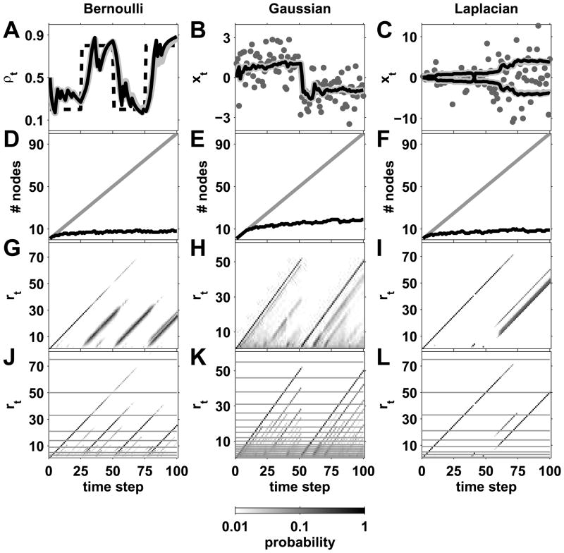
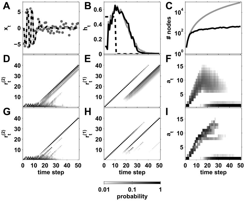
Equation 32 implies that we can prune M nodes down to $min\left[\frac{logM}{log(1+\mathrm{\Delta })},M\right]$ nodes with a loss of precision in the estimate of ρ that is bounded by Δ. For large M this will result in a substantial reduction in computational complexity. The left hand column of figure 5 (panels A, D, G, and J) shows the effects of the pruning algorithm on model output and computational complexity in the case of Bernoulli data.

Figure 5.

Effect of pruning on the two-level case for Bernoulli, Gaussian, and Laplacian data (columns). A–C, Generative parameters (dashed line in A), data (gray circles in B and C), and inferences from a pruned (solid black lines) and unpruned (thick gray lines) models versus time. D–F, Number of nodes versus time for the pruned (black) and unpruned (gray) cases. G–I, Unpruned run-length distribution versus time. J–L, Pruned run-length distributions versus time. Horizontal lines indicate bin boundaries used for pruning.

5.1.2 Generalization beyond Bernoulli distribution

Similar results can be found for more general distributions with the proviso that the constraints are probabilistic. In particular, we consider the change in mean across a bin of size δ between run-lengths r₁ and r₂. The mean at r₂ is given by

$$\mu (r_2)=\frac{1}{r_2+v_p}\left(\sum _{i=t-r_2+1}^t{x}_i+{\chi }_0\right)$$ (33)

where χ₀ and v_p are parameters of the prior distribution. Note that in this section we only consider scalar data. A similar analysis for the vector case yields similar constraints on the magnitude of the p change in mean across the bin size, with the only difference being a factor of $\sqrt{d}$, where d is the dimensionality of the data.

Because the data, x_i, in the general case might not be bounded, we can no longer give hard constraints for the maximum and minimum values for the mean at run-length r₁ given the sufficient statistics at r₂. However, if we introduce a variable S that describes the scale of the prior distribution over x_i, then we can introduce probabilistic constraints. Specifically, if we choose S to describe the scale of the data, {x_i}, containing some large fraction, f (e.g. = 0.99), of the probability mass of the prior, then we can say that with probability of at least f, that μ(r₁) will be bounded between μ(r₁)₊ and μ(r₁)₋ which are given by:

$$\mu {(r_1)}_{\pm }=\frac{1}{r_2+v_p-\delta }\left(\sum _{i=t-r_2+1}^t{x}_i\pm S\delta +{\chi }_0\right).$$ (34)

If we define the two possible changes in mean across the bin, Δ₊ and Δ₋ as

$${\mathrm{\Delta }}_{+}=\mu {(r_1)}_{+}-\mu (r_2)\text{and}{\mathrm{\Delta }}_{-}=\mu (r_2)-\mu {(r_1)}_{-}$$ (35)

then we can write

$${\mathrm{\Delta }}_{\pm }=\frac{(S\pm \mu (r_2))\delta }{r_2+v_p-\delta }$$ (36)

By definition, with probability f

$$-S\le \mu (r_2)\le S$$ (37)

Therefore, with probability f, we have

$${\mathrm{\Delta }}_{\pm }\le \mathrm{\Delta }=\frac{2S\delta }{r_2+v_p-\delta }$$ (38)

Dividing through by 2S gives

$$\frac{\delta }{r_2+v_p-\delta }=\frac{\mathrm{\Delta }}{2S}=k$$ (39)

which is reminiscent of equation 30. Indeed if we require that this fraction, k, is constant, then we find that

$$\delta =\frac{(r_2+v_p)k}{1+k}=k(r_1+v_p)$$ (40)

which gives that

$$log(r_2+v_p)-log(r_1+v_p)=log(1+k)$$ (41)

Thus log(r + v_p) is binned uniformly into bins of size log(1 + k) which has the effect of reducing M nodes down to $O\left[\frac{log(M+v_p)}{log(1+k)}\right]$. The center and right columns of figure 5 show the effects of the pruning algorithm on change-point data with Gaussian and Laplacian generative data.

5.2 Node pruning in a three-level hierarchy

In the three-level case, the similarity between nodes is based on not only the low-level run-length, r⁽²⁾, but also the high-level run-length, r⁽¹⁾, and the node’s estimate of the hazard rate, h̃ (Note that we have reintroduced the superscript notation, r⁽²⁾ for the low-level run-length and r⁽¹⁾ for the high-level run-length to avoid ambiguity). The variables r⁽¹⁾ and h̃ relate to the change-point and non-change-point counts, a and b introduced in section 4.2, via

$$r^{(1)}=a+b$$ (42)

$$\stackrel{\sim }{h}=\frac{a+a_p}{r^{(1)}+a_p+b_p}$$ (43)

As before, we grid the low-level run-length, r⁽²⁾, space logarithmically; i.e., log(r⁽²⁾ + v_p) is uniformly binned into bins of size log(1 + k⁽²⁾), where we have introduced the superscript ⁽²⁾ on k for clarity. A similar approach is also valid for the high-level run-length r⁽¹⁾: we can bin log(r⁽¹⁾ + a_p + b_p) into bins of size log(1 + k⁽¹⁾), then use k⁽¹⁾ as the bin size for h̃. Figure 6 shows an example on the effects of pruning in a three-level hierarchy.

Figure 6.

Effect of pruning on a three-level hierarchy example. A The data (circles) are sampled from a Gaussian distribution whose mean changes every 2 time steps for t ≤ 10 and then remains constant afterwards. The predictive mean is shown for the unpruned (dashed black) and pruned (gray) model. B The model’s estimates of h (gray line unpruned, black line pruned) compared with the generative h (dashed black line). C The number of nodes for the unpruned (gray) and pruned (black) cases over time on a logarithmic scale. D Marginal low-level run-length distribution, $p(r_t^{(2)}\mid x_{1:t})$, in the unpruned case. This is to be compared with the pruned version of the same distribution in panel G. E and H Marginal high-level run-length distribution, $p(r_t^{(1)}\mid x_{1:t})$, in the unpruned and pruned cases respectively. F and I Marginal change-point count distribution, p(a_t|x_1:t), in the unpruned and pruned cases.

6 Simulations

In this section we demonstrate the applicability of the algorithm by testing it on three different data sets. The main motivation in developing our model was as an ideal observer for rule-switching and other change-point tasks used in numerous behavioral, neurophysiological, and neuroimaging studies (Behrens et al., 2007; Steyvers and Brown, 2006; Brown and Steyvers, 2009; Yu and Dayan, 2005; Lau and Glimcher, 2005; Berg., 1948; Corrado et al., 2005; Averbeck and Lee, 2007; Sugrue et al., 2004). Therefore, the first two examples demonstrate how our algorithm aids the understanding of specific, published experiments. As an additional example, we show how the model can be used to find high-level change-point structure in real-world stock-market data.

6.1 Inference of a time-varying reward rate

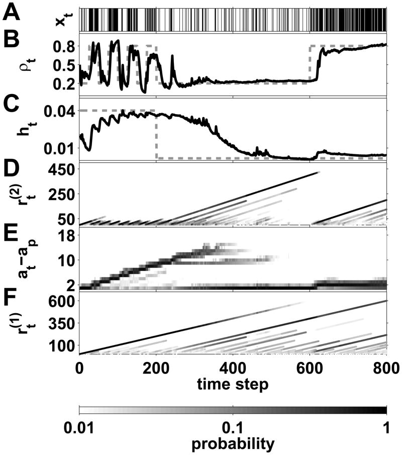
In (Behrens et al., 2007), human subjects were were engaged in a task that required tracking the rate of a Bernoulli process given binary input (i.e., reward or no reward) as in figure 7A. As shown in figure 7B, this Bernoulli rate, ρ_t undergoes a series of change-points. Moreover, the rate of these change-points varies over time, starting from an initial ‘volatile’ phase in which change-points occur every 25 time steps or so and then moving into a stable phase in which there is only one change-point in about 600 time steps.

Figure 7.

Bernoulli data example, similar to that in (Behrens et al., 2007). A. Binary data representing the presence (vertical black line) or absence (vertical white line) of reward at a given time. B. The probability of reward delivery, ρ_t, (gray dashed line) changes over time according to a change-point process and is well tracked by the algorithm (black line). C The actual hazard rate over time (dashed gray line) compared with the hazard rate inferred by the model (black line). D The low level run-length distribution, p(r⁽²⁾|x_1:t) computed by the model as a function of time. E The change-point count distribution, p(a_t|x_1:t), as a function of time. F The high level run-length distribution, p(r⁽¹⁾|x_1:t), as a function of time shows that the model has recognized the high level change-point at t = 200.

In (Behrens et al., 2007) the authors developed an approximate model for inference in this system in which they assumed random-walk dynamics for the reward rate. They then analyzed fMRI data for correlates of the parameters in their model, thus mapping the abstract computation onto a network of brain structures. However, because their model cannot capture the abrupt changes that are present in their behavioral experiment, it is not, in fact, the ideal observer. In contrast, our model was developed explicitly to identify these abrupt changes. Consequently, a three-level hierarchical model with a Bernoulli data generative distribution is the ideal-observer model for this experiment and may be better suited for functional imaging analysis. An additional advantage of our model is that, by changing the data generative distribution to (for example) Gaussian, it can also deal with continuous instead of binary reward values.

As shown in figure 7, our model does an excellent job of tracking both the reward rate (figure 7B) and, with a slightly longer lag, the hazard rate h_t (7C) over time. This lag is a consequence of the fact that the hazard rates in this model are fairly low and that it takes on the order of 1/(Δρ) binary data points to distinguish between Bernoulli generative processes with rates differing by Δρ. These effects results from the model’s ability to identify both low- and high-level change-points (7D–F).

6.2 Prediction of a time-varying position

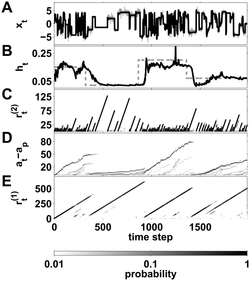
In figure 8 we demonstrate the ability of the algorithm to deal with a change-point task that is an extension of (Steyvers and Brown, 2006). In this task, subjects are asked to to try to predict the next location of a stimulus whose position is determined by a sampling from a Gaussian distribution whose mean and variance change randomly at change-points whose locations are sampled from a Bernoulli distribution with a time-varying hazard rate.

Figure 8.

Gaussian example. A The data over time (thin gray line) are sampled from a Gaussian distribution whose mean and variance undergo change-points. The black line indicates the model’s estimate of the predictive mean. B The model’s estimate of the hazard rate (black line) compared with the true hazard rate of the generative process (dashed gray line). C The low level run-length distribution, $p(r_t^{(2)}\mid x_{1:t})$ over time. D The change-point count distribution, p(a_t − a_p|x_1:t) over time. E The high level run-length distribution, $p(r_t^{(1)}\mid x_{1:t})$.

In (Steyvers and Brown, 2006), the authors also developed an ideal-observer model of this task that assumed a fixed hazard rate, was offline, and was based on Monte Carlo sampling of the posterior distributions. In contast, our approach allows us to compute optimal online behavior in more challenging environments in which the hazard rate changes over time.

As in the Bernoulli example, a three-level hierarchy model with node pruning does a good job of tracking both the data (figure 8A) and, with a slightly longer lag, the underlying hazard rate (8B) over time. These effects result from the model’s ability to identify both low- and high-level change-points (8C–E).

Figure 8A shows the input (gray line) and the predictive mean (black line) computed by the algorithm, which clearly follows the data quite faithfully. The same can be said of the model’s estimate of the hazard rate (black line - panel B) which closely follows the true, underlying hazard rate (dashed gray line).

6.3 Returns on General Motors stock

To demonstrate the general applicability of the model, we used it to analyze the daily returns from General Motors (GM) stock from January 10th, 1972, to December 23rd, 2009. Following (Adams and MacKay, 2007), we compute the log daily returns as

$$R_t=log\left(\frac{p_t^{\text{close}}}{p_{t-1}^{\text{close}}}\right)$$ (44)

where $p_t^{\text{close}}$ is the closing price on day t. We model this as being sampled from a zero-mean Laplace distribution with a variable scale factor, λ; i.e., between two change-points, R_t is sampled from

$$R_t\sim \frac{1}{Z}exp\left(-\frac{\mid R_t\mid }{{\lambda }_t}\right)$$ (45)

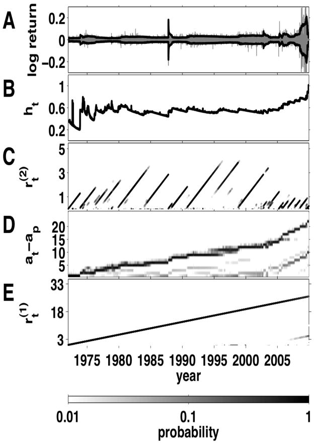
The results of running the model on this data are shown in figure 9. The model tracks the log daily returns faithfully (figure 9A). This tracking is based on an estimate of the hazard rate that changed over time, in particular showing an increase in the frequency of low-level change-points towards the end of the time series. This effect reflected shorter low-level run-lengths starting around 2001, implying a high-level change-point at that time. It is fun to observe, although by no means a strong causal statement, that this time is not long after the appointment of Richard Wagoner as CEO in June 2000. Accordingly, the model’s estimate of the hazard rate shows a marked increase towards the end of the simulation, when the high-level change-point at 2000 becomes apparent (panel B). Note that this higher-order structure in the data cannot be revealed without the hierarchical change-point model

Figure 9.

Change-point analysis of daily GM stock returns, 1972–2009. A. Daily log return (R_t, (gray line) and the estimated scale factor (λ_t, black line) from equation 44 plotted as a function of time. B. The model’s estimate of the hazard rate, ${\stackrel{\sim }{h}}_t^{(1)}$, in units of change-points per year, versus time. C. Low level run-length distribution, $p(r_t^{(2)}\mid {\mathbf{x}}_{1:t})$, versus time (note that run-length is measured in years). Several change-points are evident, corresponding to abrupt changes in the variance of the return. D. Distribution over the number of change-points, p(a_t − a₀|x_1:t), versus time. E. High level run-length distribution, $p(r_t^{(1)}\mid {\mathbf{x}}_{1:t})$, versus time. The model identified one high level change-points around 2001, roughly at the time of Richard Wagoner’s appointment as CEO. This event was followed by a higher frequency of inferred change-points and therefore an increase in the estimated hazard rate.

7 Conclusion

We introduced a novel Bayesian model for on-line inference of change-points from noisy data streams. Unlike previous approaches, our model does not require the rate of occurrence of change-points, known as the hazard rate, to be specified in advance. Rather, our model generates on-line estimates of the hazard rate itself, which then can be used to help identify change-points. The novelty of our approach rests primarily on a “change-point hierarchy” in which the hazard rate is governed by an arbitrary number of higher-order change-point processes. Thus, the model can infer hazard rates that can change with arbitrary complexity. This approach also includes a novel pruning algorithm that dramatically reduces the computational complexity of this and related models. The model is an ideal observer for several different psychophysics paradigms and has applications to real world data sets such as stock prices.

References

- Adams RP, MacKay DJ. Technical report. University of Cambridge; Cambridge, UK: 2007. Bayesian online changepoint detection. [Google Scholar]
- Aroian LA, Levene H. The effctiveness of quality control charts. Journal of the American Statistical Association. 1950;45(252):520–529. [Google Scholar]
- Averbeck BB, Lee D. Prefrontal neural correlates of memory for sequences. Journal of Neuroscience. 2007;27(9):2204–2211. doi: 10.1523/JNEUROSCI.4483-06.2007. [DOI] [PMC free article] [PubMed] [Google Scholar]
- Barlow J, Creutzfeldt O, Michael D, Houchin J, Epelbaum H. Automatic adaptive segmentation of clinical eegs. Electroencephalography and Clinical Neurophysiology. 1981;51:512–525. doi: 10.1016/0013-4694(81)90228-5. [DOI] [PubMed] [Google Scholar]
- Barry D, Hartigan JA. A bayesian analysis for change point problems. Journal of the American Statistical Association. 1993;88(421):309–319. [Google Scholar]
- Behrens TEJ, Woolrich MW, Walton ME, Rushworth MFS. Learning the value of information in an uncertain world. Nature Neuroscience. 2007;10(9):1214–1221. doi: 10.1038/nn1954. [DOI] [PubMed] [Google Scholar]
- Berg EA. A simple objective technique for measuring flexibility in thinking. J Gen Psychol. 1948;39:15–22. doi: 10.1080/00221309.1948.9918159. [DOI] [PubMed] [Google Scholar]
- Bodenstein G, Praetorius HM. Feature extraction from the electroencephalogram by adaptive segmentation. Proceedings of the IEEE. 1977;65(5):642–652. [Google Scholar]
- Brown SD, Steyvers M. Detecting and predicting changes. Cognitive Psychology. 2009;58:49–67. doi: 10.1016/j.cogpsych.2008.09.002. [DOI] [PubMed] [Google Scholar]
- Chen J, Gupta AK. Testing and locating variance changepoints with application to stock prices. Journal of the American Statistical Association. 1997;92(438):739–747. [Google Scholar]
- Chib S. Estimation and comparison of multiple change-point models. Journal of Econometrics. 1998;86:221–241. [Google Scholar]
- Corrado GS, Sugrue LP, Seung HS, Newsome WT. Linear-nonlinear-poisson models of primate choice dynamics. Journal of Experimental Analysis of Behavior. 2005;84(3):581–617. doi: 10.1901/jeab.2005.23-05. [DOI] [PMC free article] [PubMed] [Google Scholar]
- Denison DGT, Holmes CC. Bayesian partitioning for estimating disease risk. Biometrics. 2001;57:143–149. doi: 10.1111/j.0006-341x.2001.00143.x. [DOI] [PubMed] [Google Scholar]
- Fearnhead P. Exact and efficient bayesian inference for multiple changepoint problems. Stat Comput. 2006;16:203–213. [Google Scholar]
- Fearnhead P, Liu Z. On-line inference for multiple changepoint problems. Journal of the Royal Statistical Society: Series B (Statistical Methodology) 2007;69(4):589–605. [Google Scholar]
- Green PJ. Reversible jump markov chain monte carlo computation and bayesian model determination. Biometrika. 1995;82(4):711–32. [Google Scholar]
- Hsu DA. Tests for variance shift at an unknown time point. Applied Statistics. 1977;26(3):279–284. [Google Scholar]
- Koop GM, Potter SM. Technical report. Federal Reserve Bank; New York: 2004. Forecasting and estimating multiple change-point models with and unknown number of change points. [Google Scholar]
- Lau B, Glimcher PW. Dynamic response-by-response models of matching behavior in rhesus monkeys. Journal of the Experimental Analysis of Behavior. 2005;84(3):555–579. doi: 10.1901/jeab.2005.110-04. [DOI] [PMC free article] [PubMed] [Google Scholar]
- Liu JS, Lawrence CE. Bayesian inference on biopolymer models. Bioinformatics. 1999;15(1):38–52. doi: 10.1093/bioinformatics/15.1.38. [DOI] [PubMed] [Google Scholar]
- Paquet U. Empirical bayesian change point detection. 2007 http://www.ulrichpaquet.com/notes/changepoints.pdf.
- Smith AFM. A bayesian approach to inference about a change-point in a sequence of random variables. Biometrika. 1975;62(2):407–416. [Google Scholar]
- Stephens DA. Bayesian retrospective multiple-changepoint identification. Applied Statistics. 1994;43(1):159–178. [Google Scholar]
- Steyvers M, Brown S. Prediction and change detection. In: Weiss Y, Scholkopf B, Platt J, editors. Advances in Neural Information Processing Systems. Vol. 18. MIT Press; 2006. pp. 1281–1288. [Google Scholar]
- Sugrue LP, Corrado GS, Newsome WT. Matching behavior and the representation of value in the parietal cortex. Science. 2004;304:1782–1787. doi: 10.1126/science.1094765. [DOI] [PubMed] [Google Scholar]
- Wainwright MJ, Jordan MI. Graphical models, exponential families, and variational inference. Foundations and Trends in Machine Learning. 2008;1(1–2):1–305. [Google Scholar]
- Xuan X, Murphy K. Modeling changing dependency structure in multivariate time series. 24th International Conference on Machine Learning.2007. [Google Scholar]
- Yu AJ, Dayan P. Uncertainty, neuromodulation, and attention. Neuron. 2005;46(4):681–692. doi: 10.1016/j.neuron.2005.04.026. [DOI] [PubMed] [Google Scholar]
Associated Data
This section collects any data citations, data availability statements, or supplementary materials included in this article.