Automated Sulci Identification via Intrinsic Modeling of Cortical Anatomy

Abstract

In this paper we propose a novel and robust system for the automated identification of major sulci on cortical surfaces. Using multiscale representation and intrinsic surface mapping, our system encodes anatomical priors in manually traced sulcal lines with an intrinsic atlas of major sulci. This allows the computation of both individual and joint likelihood of sulcal lines for their automatic identification on cortical surfaces. By modeling sulcal anatomy with intrinsic geometry, our system is invariant to pose differences and robust across populations and surface extraction methods. In our experiments, we present quantitative validations on twelve major sulci to show the excellent agreement of our results with manually traced curves. We also demonstrate the robustness of our system by successfully applying an atlas of Chinese population to identify sulci on Caucasian brains of different age groups, and surfaces extracted by three popular software tools.

1 Introduction

The automated identification of major sulci on the human cortex is a challenging problem with important applications in brain mapping[1]. While their form and location can vary quite significantly, there is no difficulty for an anatomist to observe the regularity of major sulci based simply on the geometry of cortical surfaces regardless of their size, orientation, and the software used to extract them from MRI images. From an engineering point of view, this simplicity is critical for a computational system to achieve the same level of robustness, which essentially lies in its ability of modeling sulcal anatomy with the geometry of cortical surfaces. To this end, we propose in this work a novel system for automated sulci identification by integrating local geometry, i.e., curvature, with global descriptors derived from the Laplace-Beltrami eigen-system [2,3,4] and intrinsic surface mapping [5].

At the core of our system is an intrinsic atlas of major sulci that represents prior knowledge in training data and enables the integration of curvature information into major sulci. This atlas-based approach is most related to learning-based methods for sulci identification in previous work [6,7,8,9,10]. Principal component analysis were used to model sulcal basins [6] and sulcal lines on the sphere [7]. Boosting methods were used in [9,10]. The Markovian relation of multiple sulci was incorporated with graphical models [8,10]. The main novelty in our system is that the modeling of cortical anatomy is based entirely on intrinsic geometry, which eliminates the use of coordinates in conventional MRI atlases such as the Talairach atlas. This makes our system robust to pose differences and variations across populations. We demonstrate this robustness by using an atlas constructed from a Chinese population to detect twelve major sulci on Caucasian brains of different age groups and surfaces extracted by different software tools.

The rest of the paper is organized as follows. In section 2, we describe the construction of the intrinsic atlas for the modeling of sulcal anatomy. The sulci identification algorithm based on this atlas is developed in section 3. Experimental results are presented in section 4. Finally conclusions are made in section 5.

2 Atlas Construction

As illustrated in Fig. 1, there are two main steps in the construction of the atlas. In the first step, a multiscale representation of the cortical surface is constructed. In the second step, surface maps at a selected scale are computed to bring manually traced sulcal lines to an atlas surface. We describe the two steps in detail next.

Fig. 1.

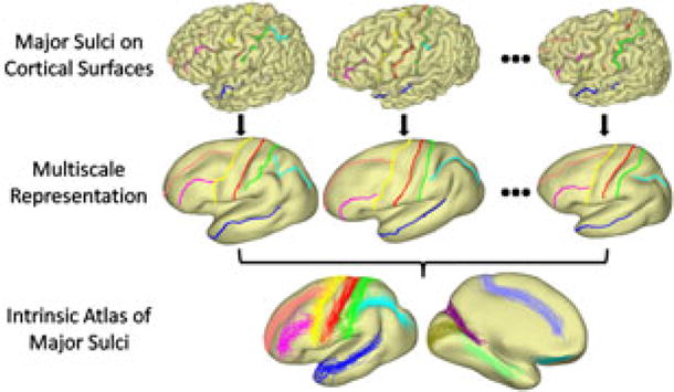
Atlas construction

2.1 Multiscale Surface Representation

Let = (, ) denote the triangular mesh representation of a cortical surface, where and are the set of vertices and triangles. We construct the multiscale representation of by using the eigen-system of its Laplace-Beltrami operator , which is defined as

$${\mathrm{\Delta }}_{\mathcal{M}}f=-\lambda f.$$ (1)

The spectra of is discrete and we denote the eigenvalues as λ₀ ≤ λ₁ ≤ · · · and the corresponding eigenfunctions as f₀, f₁, · · ·. To numerically compute the eigenfunctions, we use the finite element method and solve a generalized matrix eigenvalue problem[2,3,4].

Let X(·, 0) : → ℝ³ denote the coordinate function on , i.e., X(p, 0) = p for p ∈ . Using the eigen-system, we can express the heat diffusion of the coordinate function as

$$X(\mathbf{p},t)=\sum _{n=0}^{\infty }{e}^{-{\lambda }_{n}t}{f}_n(\mathbf{p}){\int }_{\mathcal{M}}{f}_n(\mathbf{q})X(\mathbf{q},0)d\mathcal{M}$$ (2)

By replacing the coordinates of the vertices on with X(·, t), we have a multiscale representation of . For numerical implementation, we approximate the diffusion with the first 300 eigenfunctions that are computed efficiently with the spectrum shift technique [11]. As an illustration, we show in Fig. 2 the multi-scale representation of a cortical surface at the scale t = 0, 10, 100, 1000. With the increase of the scale, we can see the surface exhibits more regularity that is common across population. However, sulcal landmarks on the original surface might be overly distorted in terms of length and angle if t is too large. In our work, we usually choose t = 100 as a tradeoff between surface regularity and landmark distortion.

Fig. 2.

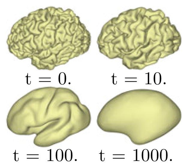
Multiscale representation of a cortical surface

2.2 Atlas Construction via Intrinsic Surface Mapping

To construct the atlas at a selected scale, we extend the intrinsic surface mapping technique developed for sub-cortical surfaces in [5] to cortical surfaces. Given a pair of surfaces ${\mathcal{M}}_1^t$ and ${\mathcal{M}}_2^t$ at a scale t, we compute two maps $u_1:{\mathcal{M}}_1^t\to {\mathcal{M}}_2^t$ and $u_2:{\mathcal{M}}_2^t\to {\mathcal{M}}_1^t$ by minimizing the following energy:

$$E={\int }_{{\mathcal{M}}_1^t}[\sum _{j=1}^3{\alpha }_D^j{({\xi }_1^j-{\xi }_2^j\circ u_1)}^2+{\alpha }_{IC}{(I-u_2\circ u_1)}^2+{\alpha }_H{\left|\right|J_{u_1}\left|\right|}^2]d{\mathcal{M}}_1^t+{\int }_{{\mathcal{M}}_2^t}[\sum _{j=1}^3{\alpha }_D^j{({\xi }_2^j-{\xi }_1^j\circ u_2)}^2+{\alpha }_{IC}{(I-u_1\circ u_2)}^2+{\alpha }_H{\left|\right|J_{u_2}\left|\right|}^2]d{\mathcal{M}}_2^t$$ (3)

where ${\xi }_i^j(i=1,2;j=1,2,3)$ are the feature functions defined on the surfaces that characterize their intrinsic geometry. In each integral, the first term penalizes the difference of feature functions, the second term encourages inverse consistency, and the third term uses the harmonic energy [12] for smoothness regularization, where J_u1 and J_u2 are the Jacobian of the maps. The regularization parameters α_D, α_IC, α_H control the weight of different terms.

To model the sulcal anatomy intrinsically, we define three feature functions on cortical surfaces as shown in Fig. 3(a) by using the Reeb graph of the first and second eigen-function of its Laplace-Beltrami operator [5]. We can see these functions characterize the frontal-posterior, superior-inferior, and medial-lateral profile of the surface intrinsically. By projecting each point $\mathbf{p}\in {\mathcal{M}}_i^t$ to ( ${\xi }_i^1(\mathbf{p}){\xi }_i^2(\mathbf{p}){\xi }_i^3(\mathbf{p})$), we construct an embedding of each surface in the feature space. As shown in Fig. 3(b), the two cortical surfaces align much better in the embedding space, which enables us to find a good initial map between them by simply looking for the nearest point on the other surface. Starting from the initial maps, we iteratively evolve them by solving a pair of PDEs on the surfaces in the gradient descent directions [5].

Fig. 3.

(a) Intrinsic feature functions. (b) Embedding in the feature space.

By choosing one of the surface in the training set as the atlas surface, we compute the maps from all other surfaces in the training data to this atlas surface . All the manually traced sulcal lines can then be projected onto the atlas surface as shown in the third row of Fig. 1. Since both the multiscale representation and surface mapping are established via intrinsic geometry, we denote the collection of sulcal lines projected onto the atlas surface as the intrinsic atlas of major sulci.

3 Automated Identification of Major Sulci

Using the atlas of major sulci, we develop in this section an automated system for their identification on cortical surfaces. Given a new surface , the skeletal representation of its sulcal region is first computed based on the mean curvature of [13] as shown in Fig 4(a). The skeleton is decomposed into a set of branches B = {B₁, B₂, · · ·}, where each branch is a polyline on . The multiscale representation of and the map u : → is then computed. With the map u, the branches are projected onto the atlas surface and denoted as B̂ = {B̂₁, B̂₂, · · ·,}. Our goal is to extract anatomically consistent sulcal lines from these skeletal branches.

Fig. 4.

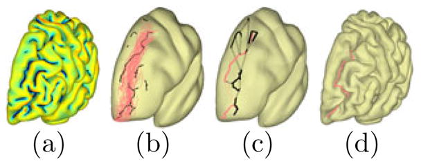
(a) Skeletal branches of the sulcal region. (b) Candidate branches (black) together with the training curves of the superior frontal sulcus. (c) Sample paths (black) and the most likely path (red). (d) The detected curve on the original surface.

Let $S_i=\{S_i^1,S_i^2,\cdots ,S_i^J\}$ denote the set of training curves for the i-th sulcus on the atlas surface. Given the prior model S_i, the challenge is how to model the likelihood of skeletal branches in B̂. The difficulty arises from the fact that B contains only partial observations of major sulci as they frequently cross gyral regions. To bridge the gap between the prior model of complete sulci and the partial observation in skeletal branches, we propose below a projection operator to model the likelihood of a branch on a major sulcus. Given a curve segment C on , its projection onto the training data S_i is defined as:

$$P_{S_i}(C)=\{y(\mathbf{x})\in S_i^j,x\in C\mid ||x-y||={min}_{z\in S_i^j}||x-z||\}$$ (4)

where $S_i^j=arg{min}_j{d}_H(C,S_i^j)$ and d_H is the Hausdorff distance. Given a branch B̂_k and its projection P_Si (B̂_k), we calculate the Hausdorff distance D_k = d_H (B̂_k, P_Si (B̂_k), and the projection ratio R_k = ||P_Si (B̂_k)||/||B̂_k||, where ||·|| denotes the length of a curve. Using the distance D_k and projection ratio R_k, we can pick a set of candidate branches as N̂ = {B̂_k ∈ B̂| D_k ≤ T HD₁, R_k ≥ T HD₂} where T HD₁ and T HD₂ are thresholds which we choose as 15mm and 0.5 in our practice. The candidate branches are plotted together with the training set over the atlas surface in Fig. 4(b).

Using the candidate branches in N̂, we construct a directed graph to generate a set of sample paths on as candidate curves for the sulcus. Given two nodes B̂_p and B̂_q in N̂, whose points are ordered according to the indices of their projection on S_i, we form a new curve C_p,q = (B̂_p, B̂_q) by connecting the end point ${\widehat{B}}_p^e$ of B̂_p with the start point ${\widehat{B}}_q^s$ of B̂_q. Once again we compute the projection of C_p,q onto S_i to evaluate the likelihood of B_p and B_q belonging to the same sulcus. Let D_p,q and R_p,q denote the distance and projection ratio of C_p,q. If R_p,q ≥ T HD₂, we add an edge from B̂_p to B̂_q and define the weight as $\frac{1}{D_{p,q}\left|\right|{\widehat{B}}_p^e-{\widehat{B}}_q^s\left|\right|}$, where the distance $\left|\right|{\widehat{B}}_p^e-{\widehat{B}}_q^s\left|\right|$ is included to encourage the connection of close branches. Starting from any branch without parents, we perform random walks on the graph to generate sample paths on the atlas surface. The probability of taking an edge during any walk is in proportion to its weight.

Let $C_i=\{C_i^1,C_i^2,\cdots \}$ be the set of sample paths for the i-th sulcus. For a candidate curve, its distance to the training data is defined as:

$$d(C_i^k;S_i)=\underset{j}{min}(\overline{d}(C_i^k,S_i^j)+\overline{d}(S_i^j,C_i^k))$$ (5)

where d̄(·, ·) is the average distance from points on a curve to the other curve. We also define the “sulcality” of each curve as:

$$\mathit{Sulcality}(C_i^k)={\sum }_{{\widehat{B}}_p\subset C_i^k}\left|\right|{\widehat{B}}_p\left|\right|/\left|\right|C_i^k\left|\right|$$ (6)

which measures how good the path follows the sulcal regions. We then define the likelihood of each curve as

$$\mathcal{L}(C_i^k\mid S_i)=e^{-d(C_i^k;S_i)/\mathit{Sulcality}(C_i^k)}$$ (7)

and choose the detection result as the sample curve in C_i with the maximum likelihood. As an illustration, we show on the set of sample paths and the path with the maximum likelihood for the superior frontal sulcus in Fig. 4(c). The branches in this path are then connected via a curvature-weighted geodesic on the original surface to obtain the detected sulcus as plotted in Fig. 4(d).

Let C_i1 and C_i2 denote the candidate curves of the i1-th and i2-th sulcus, we define the joint distance from a pair of curves $C_{i1}^p\in C_{i1}$ and $C_{i2}^q\in C_{i2}$ to the training curves S_i1 and S_i2 as:

$$d(C_{i1}^p,C_{i2}^q;S_{i1},S_{i2})=\underset{j}{min}(\overline{d}(C_{i1}^p,S_{i1}^j)+\overline{d}(S_{i1}^j,C_{i1}^p)+\overline{d}(C_{i2}^q,S_{i2}^j)+\overline{d}(S_{i2}^j,C_{i2}^q))$$ (8)

The joint likelihood of the two curves is then defined as:

$$\mathcal{L}(C_{i1}^p,C_{i2}^q\mid S_{i1},S_{i2})=e^{-d(C_{i1}^p,C_{i2}^q;S_{i1},S_{i2})/(\mathit{Sulcality}(C_{i1}^p)\ast \mathit{Sulcality}(C_{i2}^q))}$$ (9)

The joint detection results are the pair of curves in the sample space C_i1 × C_i2 achieving the maximum likelihood.

4 Experimental Results

In this section, we present experimental results on four different datasets, including surfaces extracted from 3 software tools, to demonstrate our sulci detection system.

4.1 Atlas Construction and Quantitative Validation

In the first experiment, we applied our method to pial surfaces extracted from the 3T MRI images of 65 Chinese young subjects (18 ~ 27 years) by Freesurfer [14]. The left hemispheres were used in this work. Twelve major sulci as listed in Table 1 were manually traced on each surface. We used 40 surfaces as training data to construct the intrinsic atlas of major sulci, which is shown on the third row of Fig. 1, and the algorithm developed in section 3 was used to identify the twelve major sulci on the other 25 surfaces for testing and quantitative validation. For robustness, the central and post-central sulcus were detected jointly by maximizing the joint likelihood in (9). The other 10 sulci were detected separately by maximizing the likelihood in (7).

Table 1.

Quantile statistics in testing data. (S₁:central; S₂:post-central; S₃:pre-central; S₄:superior-temporal; S₅:intraparietal; S₆:inferior-frontal; S₇:superior-frontal; S₈:olfactory; S₉:collateral; S₁₀:parietal-occipital; S₁₁:cingulate; S₁₂:calcarine.)

		S1	S2	S3	S4	S5	S6	S7	S8	S9	S10	S11	S12
dam(mm)	70%	3.2	5.1	3.6	3.6	3.5	5.2	3.6	3.0	4.7	1.7	3.7	1.7
	80%	3.6	8.2	4.8	4.8	4.6	8.2	5.6	3.3	6.6	2.3	5.1	2.1
	90%	5.2	11.1	7.7	8.4	8.0	10.2	8.7	4.2	8.9	4.4	7.7	3.8
dma (mm)	70%	3.6	6.6	5.5	4.2	4.4	8.0	4.7	3.3	5.7	2.2	4.6	3.9
	80%	4.6	9.3	7.8	6.4	6.5	9.8	6.9	3.7	7.7	3.4	6.9	7.3
	90%	7.1	12.3	11.2	10.6	10.1	11.7	10.2	5.1	11.2	6.0	9.2	11.5

As an illustration, the results from 4 subjects in the testing data are plotted in Fig. 5. For better visualization, we plotted the detected curves on the surfaces at the scale t = 10 in Fig. 5(a) and (b). As shown in Fig. 5(c), the automatically detected sulcal lines align very well with manually traced sulci plotted in black. Quantile statistics of two distances d_am and d_ma of each sulcus were listed in Table 1, where d_am is the distance from points on a detected curve to the corresponding manually traced curve, and d_ma denotes the distance from points on each manual curve to the detected sulcus. For example, the first number in the column of S₁ means that 70% of the points on the automatically identified central sulcus are within a distance of 3.2mm to the manually traced curve. While there is variability across different sulci, we can see the quantile statistics show the automated results accurately capture the main body of the major sulci.

Fig. 5.

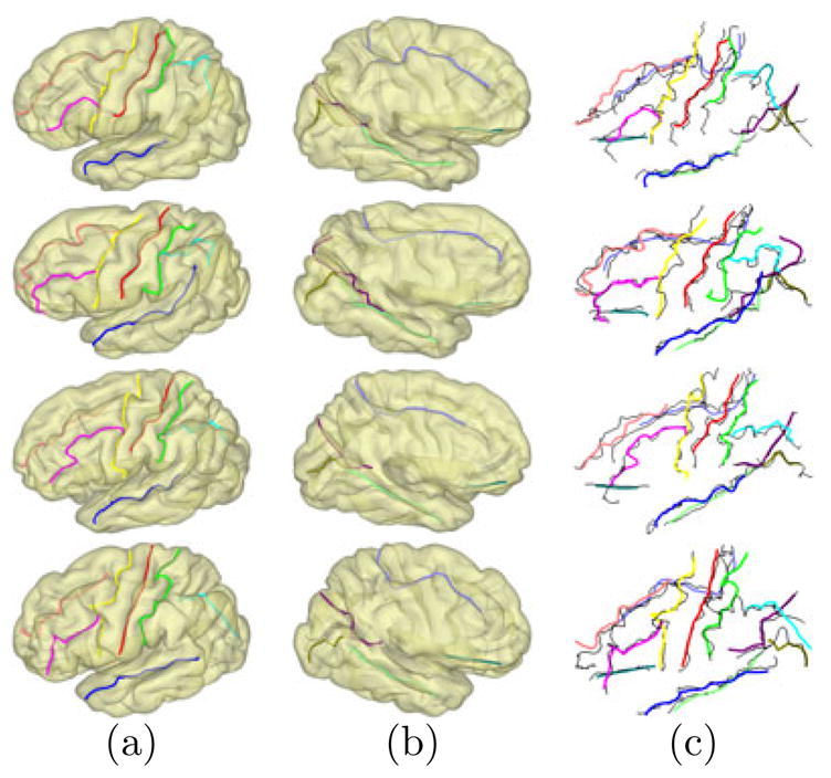
Detection results on testing data. (a) Lateral view. (b) Medial view. (c) Overlay with manually traced curves (black).

4.2 Robustness

In the second experiment, we applied the atlas built from the Chinese population in the first experiment to detect sulci on three different datasets of Caucasian brains. The first dataset consists of the left pial surfaces of eight elderly subjects (63 ~ 85 years) extracted by Freesurfer. The second dataset is composed of the left pial surfaces of two young adults extracted by BrainSuite [15]. The third dataset consists of white matter surfaces of two young adults extracted by BrainVisa [16]. For better visualization, we also plot the detected curves on all surfaces at the scale t = 10 in Fig. 6. These results demonstrate the robustness of our method across ethnic and age groups, and different software tools for surface extraction.

Fig. 6.

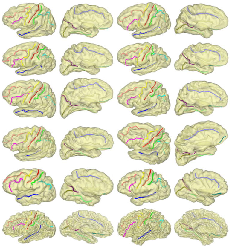
Row 1–4: results on elderly subjects. Row 5: results on BrainSuite surfaces. Row 6: results on BrainVisa surfaces.

5 Conclusion

In summary, we have developed a novel system for the automated detection of major sulci on cortical surfaces. Quantitative validations on twelve major sulci showed excellent agreement between our system and manual tracing. We also demonstrated the robustness of our system across different populations and surface extraction tools. For future work, we will augment our system with the intrinsic modeling of gyral landmarks to further improve its performance.

References

- 1.Thompson PM, et al. Mapping cortical change in alzheimers disease, brain development, and schizophrenia. NeuroImage. 2004;23:S2–S18. doi: 10.1016/j.neuroimage.2004.07.071. [DOI] [PubMed] [Google Scholar]
- 2.Qiu A, Bitouk D, Miller MI. Smooth functional and structural maps on the neocortex via orthonormal bases of the Laplace-Beltrami operator. IEEE Trans Med Imag. 2006;25(10):1296–1306. doi: 10.1109/tmi.2006.882143. [DOI] [PubMed] [Google Scholar]
- 3.Reuter M, Wolter F, Peinecke N. Laplace-Beltrami spectra as Shape-DNA of surfaces and solids. Computer-Aided Design. 2006;38:342–366. [Google Scholar]
- 4.Shi Y, et al. Anisotropic Laplace-Beltrami eigenmaps: Bridging Reeb graphs and skeletons. Proc MMBIA. 2008:1–7. doi: 10.1109/CVPRW.2008.4563018. [DOI] [PMC free article] [PubMed] [Google Scholar]
- 5.Shi Y, et al. Inverse-consistent surface mapping with Laplace-Beltrami eigen-features. Proc IPMI. 2009:467–478. doi: 10.1007/978-3-642-02498-6_39. [DOI] [PMC free article] [PubMed] [Google Scholar]
- 6.Lohmann G, Cramon D. Automatic labelling of the human cortical surface using sulcal basins. Med Image Anal. 2000;4:179–188. doi: 10.1016/s1361-8415(00)00024-4. [DOI] [PubMed] [Google Scholar]
- 7.Tao X, Prince J, Davatzikos C. Using a statistical shape model to extract sulcal curves on the outer cortex of the human brain. IEEE Trans Med Imag. 2002;21(5):513–524. doi: 10.1109/TMI.2002.1009387. [DOI] [PubMed] [Google Scholar]
- 8.Rivière D, et al. Automatic recognition of cortical sulci of the human brain using a congregation of neural networks. Med Image Anal. 2002;6:77–92. doi: 10.1016/s1361-8415(02)00052-x. [DOI] [PubMed] [Google Scholar]
- 9.Tu Z, et al. Automated extraction of the cortical sulci based on a supervised learning approach. IEEE Trans Med Imag. 2007;26:541–552. doi: 10.1109/TMI.2007.892506. [DOI] [PubMed] [Google Scholar]
- 10.Shi Y, et al. Joint sulcal detection on cortical surfaces with graphical models and boosted priors. IEEE Trans Med Imag. 2009;28(3):361–373. doi: 10.1109/TMI.2008.2004402. [DOI] [PMC free article] [PubMed] [Google Scholar]
- 11.Vallet B, Lèvy B. Spectral geometry processing with manifold harmonics. Computer Graphics Forum. 2008;27(2):251–260. [Google Scholar]
- 12.Mèmoli F, Sapiro G, Osher S. Solving variational problems and partial differ-ential equations mapping into general target manifolds. Journal of Computational Physics. 2004;195(1):263–292. [Google Scholar]
- 13.Shi Y, et al. Hamilton-Jacobi skeleton on cortical surfaces. IEEE Trans Med Imag. 2008;27(5):664–673. doi: 10.1109/TMI.2007.913279. [DOI] [PMC free article] [PubMed] [Google Scholar]
- 14.Dale AM, Fischl B, Sereno MI. Cortical surface-based analysis i: segmentation and surface reconstruction. NeuroImage. 1999;9:179–194. doi: 10.1006/nimg.1998.0395. [DOI] [PubMed] [Google Scholar]
- 15.Shattuck D, Leahy R. BrainSuite: An automated cortical surface identification tool. Med Image Anal. 2002;8(2):129–142. doi: 10.1016/s1361-8415(02)00054-3. [DOI] [PubMed] [Google Scholar]
- 16.Mangin JF, et al. From 3D magnetic resonance images to structural representations of the cortex topography using topology preserving deformations. Journal of Mathematical Imaging and Vision. 1995;5(4):297–318. [Google Scholar]