Characterization of the bout durations of sleep and wakefulness

Abstract

Study objectives

(a) Develop a new statistical approach to describe the microarchitecture of wakefulness and sleep in mice; (b) evaluate differences among inbred strains in this microarchitecture; (c) compare results when data are scored in 4-s versus 10-s epochs.

Design

Studies in male mice of four inbred strains: AJ, C57BL/6, DBA and PWD. EEG/EMG were recorded for 24 h and scored independently in 4-s and 10-s epochs.

Measurements and results

Distribution of bout durations of wakefulness, NREM and REM sleep in mice has two distinct components, i.e., short and longer bouts. This is described as a spike (short bouts) and slab (longer bouts) distribution, a particular type of mixture model. The distribution in any state depends on the state the mouse is transitioning from and can be characterized by three parameters: the number of such bouts conditional on the previous state, the size of the spike, and the average length of the slab. While conventional statistics such as time spent in state, average bout duration, and number of bouts show some differences between inbred strains, this new statistical approach reveals more major differences. The major difference between strains is their ability to sustain long bouts of NREM sleep or wakefulness. Scoring mouse sleep/wake in 4-s epochs offered little new information when using conventional metrics but did when evaluating the microarchitecture based on this new approach.

Conclusions

Standard statistical approaches do not adequately characterize the microarchitecture of mouse behavioral state. Approaches based on a spike-and-slab provide a quantitative description.

1. Introduction

Mice are increasingly becoming the animal model for studying sleep. The advantages of using mice are the accessibility to many inbred strains as well as recombinant inbreds to facilitate identification of quantitative trait loci. Other advantages are the availability of congenics and consomics to facilitate gene identification and large-scale ENU mutagenesis projects that have been, and are being, conducted in mice. All of these strategies are being undertaken to identify genes regulating biological processes such as sleep.

These strategies all require quantitative analysis of the phenotypes of interest. One aspect of the sleep phenotype that has received recent attention is the flip-flop control of sleep and wakefulness (Saper et al., 2005). It is argued that interaction between sleep and wake-active neurons controls whether the animal exhibits sleep or wakefulness. Within sleep there is a flip-flop switch that controls states, i.e., NREM and REM sleep (NREM is non-rapid eye movement sleep during which synchronized slow waves are recorded from the electroencephalogram. REM is rapid eye movement sleep during this stage there are flurries of eye movements and atonia of skeletal muscles). It is further argued that molecules such as orexin (hypocretin) help to stabilize this flip-flop switch (Saper et al., 2005). Loss of orexin in mice with a knockout of this gene leads to fragmentation of sleep, i.e., shorter sleep bouts (Chemelli et al., 1999). Thus, specific molecules may control not only the amount of sleep and wakefulness but also the maintenance of sleep and hence the bout length of different states.

Studies in different inbred mouse strains have shown that there are both short and long bouts of sleep and wakefulness and that these bout durations are not normally distributed (Franken et al., 1999). The number of bouts of different length varies between inbred strains (Franken et al., 1999). This basic feature of sleep/wake control is found in other mammals (Lo et al., 2004). The nature of these distributions is in part determined by voltage gated potassium channels as is revealed by studies in relevant transgenic mice (Joho et al., 2006). These different durations of bouts of sleep and wake have been analyzed using survival curve analysis (Behn et al., 2007; Blumberg et al., 2005, 2007; Diniz Behn et al., 2008; Joho et al., 2006; Lo et al., 2002, 2004; Simasko and Mukherjee, 2009). In general, survival curve analysis, plotting the percentage of a state as a function of different bout length, finds that for wakefulness a log–log plot leads to a linear description, i.e., a power-law distribution, while for sleep a semi-log plot, i.e., an exponential distribution, is best (Blumberg et al., 2005; Lo et al., 2002, 2004; Simasko and Mukherjee, 2009).

While these analyses have been helpful to describe the general nature of the distributions of sleep and wake bout lengths, they do not lend themselves to providing summary statistics to describe bout length distributions of individual mice or mouse strains. In order to provide such numerical summaries, we have utilized a different statistical approach. We use a special case of a mixture distribution termed a spike-and-slab (see Fig. 1; for further discussion of mixture distributions, see electronic supplement and Fig. S1). The spike is made up of the short bouts of a particular state while the slab is the long bouts.

Fig. 1.

An example of a spike-and-slab mixture distribution. On the upper panel, we see an unwieldy distribution composed of a large mass near one and a long, flat tail extending out to about ten. On the bottom panel, this distribution is decomposed into a “spike” component and a “slab” component. Often such distributions result from a latent factor (for an example, see Fig. S1).

Thus, in this study, we report a strategy to provide novel statistical measures of wake, NREM, and REM bout length distribution based on a spike-and-slab distribution (see Fig. 1). Graphical examination of bout durations indicates a large number of very short bouts (spike) in addition to a long right tail (slab). We further analyzed the data with respect to behavioral history, i.e., does the distribution of bout durations of NREM sleep, for example, depend on whether the mouse entered NREM sleep from wakefulness or REM sleep. We have applied this strategy to data from four inbred mouse strains, i.e., C57BL/6, AJ, DBA and PWD. We selected these inbred strains because they are on different branches of the mouse genealogical tree. We show that the new statistics that characterize the mixed distribution of bouts of short and long length bring out clear differences between these inbred strains. We argue that using these new statistics will benefit future studies evaluating sleep architecture in mice and help identify mice that have alterations in the flip-flop control of wake and sleep due to altered genetic control.

2. Methods

2.1. Animal studies

2.1.1. Mouse

Four inbred strains of male mice were used in this study: AJ (n = 10), C57BL/6J (n = 10), DBA/2J (n = 8), and PWD (n = 7), age: 10–12 weeks, weight: 18–23 g, purchased from Jackson Laboratory (Bar Harbor, ME). Mice were individually housed in Plexiglas cages (4 in. wide × 8 in. long × 12 in. high) and maintained on 12 h light/dark cycle (lights on 0700; 80 Lux at the floor of the cage) in a sound attenuated recording room, temperature 22–24 °C. Food and water were available ad libitum. Animals were acclimated to these conditions for 10–14 days before beginning any studies. All animal experiments were performed in accordance with the guidelines published in the NIH Guide for the Care and Use of Laboratory Animals and were approved by the University of Pennsylvania Animal Care and Use Committee.

2.2. EEG/EMG recording of sleep

Mice were implanted with EEG/EMG electrodes under deep anesthesia (i.p. injection of Ketamine (100 mg/kg)/Xylazine (10 mg/kg)). For EEG recordings, three stainless steel miniature screws (0–80 × 1/16, Plastics One, Inc., VA) were placed epidurally in the following locations: (1) right frontal cortex (1.7 mm lateral to midline and 1.5 mm anterior to bregma), (2) right parietal cortex (1.7 mm lateral to midline and 1 mm anterior to lambda), and (3) a reference electrode over the cerebellum (1 mm posterior lambda on the midline). Two EMG electrodes were sutured onto the dorsal surface of the nuchal muscles immediately posterior to the skull. All leads from the electrodes were connected to an 8-pin plastic connector/pedestal (Plastics One, Inc., VA) and then bonded to the skull with dental acrylic. After the bonding agent cured, the animals were connected to our signal amplifier system using a connecting cable and swivel-contact (Plastics One, Inc., VA) mounted above each cage. All mice had a 10–14 days post-surgery recovery and habituation period before beginning any recording.

EEG and EMG signals were amplified using the Neurodata amplifier system (Models M15, Astro-Med, Inc., West Warwick, RI). Signals were amplified (2000×) and conditioned using the following settings for EEG signals: low cut-off frequency (−6 dB), 0.3 Hz and high cut-off frequency (−6 dB), 30 Hz; for EMG signals: low cut-off frequency (−6 dB), 10 Hz and high cut-off frequency (−6 dB), 100 Hz. Signals were digitized at 100 Hz. All data were acquired and analyzed using Gamma software (Astro-Med, Inc., West Warwick, RI) and converted to European Data Format (EDF) for manual scoring and analysis in the Somnologica science software (Medcare).

2.3. Scoring of sleep/wake and substages of sleep

Wake, NREM and REM sleep were manually scored in both 4-s and 10-s epochs during 24-h baseline recordings. Stages were determined as follows: epochs were scored as wake when the EMG amplitude ranged from activity slightly higher than baseline during quiet wakefulness to higher amplitude activity during exploratory behavior. EEG amplitude was low with frequencies mostly above 10 Hz. NREM was characterized by high amplitude delta (1–4 Hz). EMG was constant with low amplitude activity. REM was characterized by low amplitude rhythmic theta waves (6–9 Hz) with the EMG remaining at baseline levels. We obtained complete sets of data for each mouse scoring using both 4-s and 10-s epochs, i.e., we had two sets of data for each mouse (Fig. S2 shows original EEG/EMG data in a single mouse for wake, NREM and REM sleep).

2.4. Statistical methodology

2.4.1. Modeling spike-and-slab bout durations

For this study we used statistical methods that take into account both the “spike-and-slab” nature of sleep durations that we found and the fact that bout durations are dependent on the previous state. In particular, we model the sequence of states as a generalized Markov model. The model is conceived simply as a vehicle for compressing a long sequence of sleep data into a few numerical summaries (or “sufficient statistics”) which describe the sequence and vary by strain. Hence, our main focus is on these statistics themselves rather than on the model.

For any sequence of states (X₁, X₂, X₃, …, X_T), we can decompose it into pairs of “unique states” and “durations” ((Y₁, Z₁), (Y₂, Z₂), …, (Y_N, Z_N)) where, informally, Y is the set of unique states and Z is the set of durations. Formally, we define the Y_i and Z_i inductively as follows: Y₁ = X₁, Z₁ = {max(τ)|X₁ = X₂ = … = X_τ ≠ X_τ+1,} and $Y_{i+1}=X_{Z_i+1},Z_{i+1}=\left\{\max \right(\tau )\mid X_{{\sum }_{j=1}^i{Z}_j+1}=X_{{\sum }_{j=1}^i{Z}_j+2}=\cdots =X_{{\sum }_{j=1}^i{Z}_j+\tau }\ne X_{{\sum }_{j=1}^i{Z}_j+\tau +1}\}$. For example, we can decompose the sequence (NREM, NREM, WAKE, WAKE, WAKE, NREM, NREM, REM, REM, REM, WAKE) into pairs ((NREM, 2), (WAKE, 3), (NREM, 2), (REM, 4), (WAKE, 1)).

Using this decomposition, we assume a mouse transitions from state Y_i to Y_i+1 according to a transition probability matrix A. Since there are three sleep/wake states, A is a 3 × 3 matrix; furthermore, due to the decomposition above, A has zeroes on the diagonal. We further assume Z_i~g|θ_Yi–1,Y1 where g is a probability distribution discussed below and θ_Yi–1,Y1 are parameters which depend on current and previous state label. Hence, the likelihood of any given state sequence X =(X₁, X₂, X₃, …, X_T) can be expressed as

$$\begin{array}{cc}\hfill L(X\mid ϴ)& =\prod _{i=1}^{N}P(Y_i=y_i\mid Y_{i-1}=y_{i-1})P(Z_1=z_i\mid Y_i=y_i,Y_{i-1}=y_{i-1})\hfill \\ \hfill & =\prod _{i=1}^{N}A(y_{i-1},y_i)g(z_i\mid {\theta }_{y_i,y_{i-1}})\hfill \end{array}$$

where $ϴ=\{A,\{{\theta }_{i,i-1}\left\}\right\}$.² Since the transition probability matrix A is ancillary to the discussion of bout duration modeling, we now focus on g, the duration distribution. We model g as a mixture distribution with two components: discrete point masses to accommodate the “short” durations in the spike and a probability density function (pdf) to accommodate the “long” durations in the slab. That is, we assume:

$$g(z\mid \theta )=\sum _{i=1}^k{\pi }_{i}I(z=i)+\left(1-\sum _{i=1}^k{\pi }_i\right)f(z\mid \phi ).$$

In this case, we need to specify k, the number of point masses, as well as the functional form of the pdf for f. Our parameters are θ = (π₁, …, π_k, φ) where φ parameterizes the long durations in the slab (and is potentially a vector) and the π_i are point masses which give the “spike” probability that a bout lasts exactly i epochs (i = 1 to k, where k is the upper threshold for the spike segment of distribution of durations). In this paper, we fixed k at 10 epochs (i.e., 40 s where EEG/EMG data are scored in 4-s epochs³), since this eases interpretability across mice and across strains of different mice.⁴

The long segment of the “slab” duration distribution f(z∣φ), is nicely fit by a gamma distribution (see Fig. 2). The gamma distribution is a probability distribution which is good for modeling values which are positive, particularly when the probability begins to decay after some point. It is determined by two parameters and has a density function given by the following formula:

$$f(z\mid \alpha ,\beta )=\frac{z^{\alpha -1}{\beta }^{\alpha }{e}^{-\beta z}}{\Gamma \left(\alpha \right)}$$

Fig. 2.

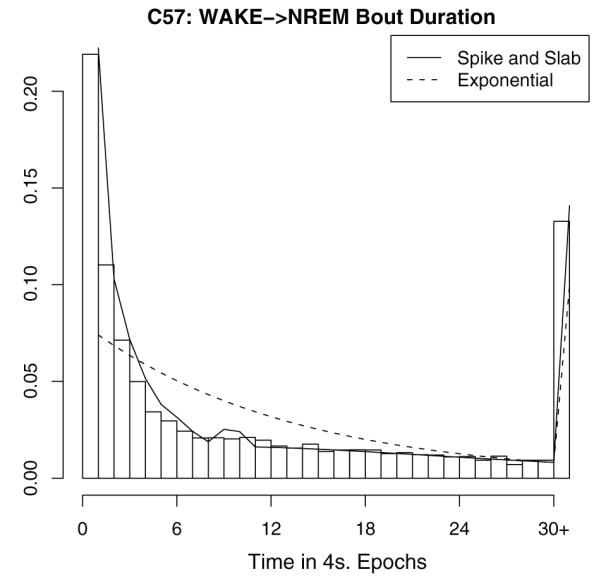
A demonstration of how a spike-and-slab distribution fits better than traditional distributions. We show C57 bout durations for NREM following from WAKE. The exponential distribution fails to capture the large spike at 1 epoch as well as the long right tail which causes a mass at thirty or more epochs. On the other hand, a spike-and-slab approach can accommodate both of these features.

It has expected value (mean) α/β and variance α/β². Since we found that the mouse’s bout duration depends on the previous state, we estimate the spike-and-slab distribution conditional on the previous state. That is, we estimate a separate distribution for five sets of bouts (e.g., WAKE from NREM, NREM from WAKE, NREM from REM, REM from NREM, and WAKE from REM).

The choice of the gamma distribution to model the long segment of the distribution was not arbitrary. In fact, there were several other candidate distributions to model the long, slab segment which we considered including the exponential, geometric, negative binomial, and pareto. We used various model selection criteria such as Chi-square likelihood-ratio tests (for nested models), the Akaike Information Criterion, the Bayesian Information Criterion, and bootstrapped Q–Q plots. The gamma distribution performed best on these tests though the negative binomial performed comparably, suggesting the choice of the underlying distribution is not so important provided it is sufficiently flexible and the spike component is included.⁵ Thus, though there is some degree of choice in the slab distribution, we found on the contrary that the spike was a sine qua non: it was strongly selected for inclusion in the model by the various criteria, regardless of the slab distribution used (see Model Selection section in the electronic supplement, Table S1, and Figs. S3 and S4 for more details).

As mentioned above, the purpose of our probability model is to generate an interpretable set of descriptive summary statistics. Taken together, our spike–slab formulation gives 12 parameters θ = (π₁, …, π₁₀, α, β) which can be further distilled into an even smaller set of three key measures:

• n The number of bouts of the sleep state conditional on the previous state.

• π The “spike” size, ${\sum }_{i=1}^{10}{\pi }_i$.

• μ The average “slab” size, α/β.

It is important to note that, for each mouse, we obtain a set of these three measures for each of the five transitions listed above. That is, each of the above three metrics is calculated for each of the three states conditional upon the value of the previous state. Hence, we have 15 total parameters in five sets (one set of three for each of the five transitions WAKE→NREM, NREM→REM, NREM→WAKE, REM→NREM, and REM→WAKE).

These summary statistics, in addition to the ones usually reported (percent of time spent in each bout, mean bout duration, and number of bouts), were used to compare mouse strains. An identical approach was used for mouse EEG/EMG data scored in 10-s epochs. For these data, k was set at 4 epochs, i.e., the maximal duration of the bouts in the spike was retained at 40 s.

2.5. Comparison of measures between strains

To compare data from the four strains, we used various statistical tests for each state–measure combination. For the conventional measures, there are nine possible combinations [three measures (amount, average bout duration, number of bouts) times three states (REM, NREM, and WAKE)]; for the new measures, introduced here, there are fifteen [three measures times five possible transitions].

To be consistent with the prior literature, we report the ANOVA F-test p-values. However, this test lacks power to truly differentiate among the strains because the ANOVA null hypothesis assumes equal means across all strains, an inappropriate benchmark when we know the strains have different underlying behavior (varied behavior implies an equal means null hypothesis is almost guaranteed to be rejected). Moreover, an F-test actually conveys little information. For example, one can have a significant F-statistic for strains while none of the individual strains show a statistically significant difference from one another. Conversely, one can have an insignificant F-statistic when several of the strains exhibit pairwise differences that are statistically significant. Moreover, the ANOVA framework requires an assumption of normality that is not appropriate in this setting. Hence, the p-values produced by F-tests are sensitive to outliers. That is, one data point (for example if one particular bout of one mouse of one strain is an outlier) can cause the p-value to shift by a large amount even if the underlying means are similar or the same.

For these reasons, we also used non-parametric pairwise tests with adjustment for multiple comparisons. In particular, we used the Wilcoxon Rank Sum Test. A non-parametric test does not rely on assumptions of normality and is far less sensitive to one or two aberrant data points. Furthermore, because they are pairwise, they assess which particular strains differ from one another.

2.6. Comparison of measures when we used a 4-s or 10-s epoch to score sleep

We also compared measures within a given strain when we scored sleep in 4-s or 10-s epochs. Again, we first used the standard ANOVA tests but also the non-parametric pairwise tests for both the standard summary statistics as well as the summary statistics arising from our new approach. Our model was fit in exactly the same way as described above. We compared the results using pairwise plots and correlation coefficient significance tests.

3. Results

3.1. Comparison of inbred strains using conventional measures

We compared each of the strains using the nine conventional measures. As can be seen in Fig. 3, the only strain that appears consistently different on these metrics is AJ. These metrics fail to show how, if at all, the other three strains differ from one another. That is, the conventional statistics lack the power to discriminate among the strains. We refer the reader to the electronic supplement for a more detailed treatment of these results, which contains statistical tests (see Tables S3 and S4) to formalize the intuition gleaned from Fig. 3.

Fig. 3.

Conventional measures for each mouse by strain. (a)–(c) Give the fraction of time for REM, NREM, and WAKE; (d)–(f) give the number of bouts; and (g)–(i) give the average bout duration in number of 4-s epochs. Means for each strain are indicated by the horizontal black line and standard errors by the vertical bars.

3.2. Examination of distribution of bout durations of behavioral states

In light of the failure of the standard statistics to provide differentiation among strains, we graphically examined the distribution of bout lengths of wake, NREM and REM sleep in each of the four mouse strains studied. We first examined the overall distribution of each state for each strain (see Fig. 4). The histograms in Fig. 4 give the state durations (scored by EEG and EMG over 4-s epochs) for mice of all strains. The histograms do not follow a nice smooth distribution that can be summarized by simple statistics. Rather, as discussed, the distributions more closely resemble a “spike-and-slab” distribution: a large “spike” near zero containing a large number of bouts whose durations are very short, along with a long “slab” corresponding to long bouts. This is illustrated by examining data for C57BL/6 (row 1 in Fig. 4).

Fig. 4.

Histograms of bout durations of each state in units of number of 4-s epochs. Duration is given on the x-axis and probability on the y-axis. (a)–(c) Give the bout durations for C57 for REM, NREM, and WAKE; (d)–(f) give the bout durations for AJ; (g)–(i) give the bout durations for DBA; (j)–(l) give the bout durations for PWD.

The first plot (left panel) in the first row of Fig. 4, which gives the bout durations for REM sleep for C57BL/6, shows a large number of bouts of length 1 and 2 epochs, i.e., 4–8 s. Beyond that, there is a long tail extending out to about 60 epochs (240 s), hence explaining the mass at 30 or more epochs. This tail decays slowly and, though it is smooth when aggregating across all mice, it is rather under populated contributing to a “jagged” decay when examined for an individual mouse. Similarly, the second plot for NREM sleep (middle of first row of Fig. 4), also has a large spike at 1 epoch. However, NREM has a “slab” which decays rather smoothly out to about 200 epochs (800 s ≈ 13 min). On the contrary, the third plot for WAKE (right panel of first row of Fig. 4), features a very prominent spike plus a rather long, flat, slab extending to over 1900 epochs (7600 s ≈ 2 h). Hence, both NREM and WAKE have extremely long right tails leading to a large mass at greater than 30 epochs in Fig. 4.

Since there are 3 sleep/wake states recognized in mice, a mouse can enter any given state (e.g., NREM sleep) from either of the other two states (in this case wake or REM sleep). We thus examined the distributions based on the recent history of specific state transitions: separate distributions of WAKE bout durations following a transition to wakefulness from NREM sleep or from REM sleep; separate distributions of bout durations of NREM sleep following transition from WAKE or REM sleep; a distribution of bout durations of REM sleep on transition from NREM sleep. We did not analyze the occasional episodes of direct transitions from wakefulness to REM (DREM) that occur occasionally in wildtype mice. These episodes occur almost exclusively during the lights on period and are the result of brief awakenings interrupting a sustained period of REM sleep (Fujiki et al., 2009). Separate conditional distributions are shown for C57BL/6 mice in Fig. 5 (the distributions for other inbred mouse strains are shown in Figs. S5–S7 in the electronic supplement). Thus, the basic nature of these distributions requires new strategies to properly characterize similarities and differences in the sleep/wake behavior of mice.

Fig. 5.

Histograms of state bout durations in units of 4-s epochs conditional on the previous state for C57. Duration is given on the x-axis and probability on the y-axis. (a) Gives the bout durations for REM followed from NREM; (b) is deliberately left empty, i.e., REM following WAKE; (c) gives the bout durations for NREM followed from REM; (d) gives the bout durations for NREM followed from WAKE; (e) gives the bout durations for WAKE followed from REM; (f) gives the bout durations for WAKE followed from NREM.

The histograms in Fig. 5 illustrate that the state bout duration variability is highly dependent on the state the mouse was in previously. For instance, a transition from REM to NREM in C57BL/6 is rarely more than about 4 epochs in length (Fig. 5(c)), whereas a transition from WAKE into NREM is “spike-and-slab” as can be seen by examining (Fig. 5(d)). That is, there is a modest probability that the bout will be short (i.e., on the spike); if it is not short (i.e., on the slab), its duration is not only much longer but it is also much more variable. Likewise, Fig. 5(e) and (f) shows that a transition into WAKE from either REM or NREM produces a “spike-and-slab”. However, much longer WAKE bouts tend to follow NREM rather than REM.

These histograms suggest that a methodology which takes into account both the conditional and spike-and-slab nature of bout duration distribution will be more successful at capturing the dynamics of sleep/wake durations. A better model will be more likely to capture nuances of various strains and thus discriminate among them. We now apply the methods outlined for our analysis of the spike-and-slab distribution to the four strains.

3.3. Comparison of inbred strains using new methodology

In Table 1, we present the mean of each of the new measures by strain and state again with ANOVA F-test statistics conducted on the strains for each of the new measures of sleep/wake state (see Figs. 6, 7, and 8 for plots). The only differences that are not statistically significant are those for the number of bouts n of REM→WAKE and the average slab size μ when the mouse transitions from REM→NREM. However, all the others are highly significant.

Table 1.

Means of each of the proposed sleep measures by strain and sleep state. The ANOVA F-statistic tests the null hypothesis of equality for all strains for each of the 15 proposed measures. p-Values between .01 and .05 are given in italics and p-values less than .01 are given in bold. Number of bouts is denoted by n, spike size is denoted by π, and average slab size is denoted by μ and is expressed in number of 4-s epochs.

Measure	State	AJ	C57	DBA	PWD	F-statistic	p-Value
n	NREM→REM	79.3	108.5	89.5	231.0	7.72	<.001
n	REM→NREM	45.4	52.4	42.6	181.6	6.21	.002
n	WAKE→NREM	1247.5	790.6	817.5	696.9	11.14	<.001
n	REM→WAKE	37.5	58.2	55.6	62.6	2.33	.093
n	NREM→WAKE	1213.6	734.5	770.6	647.4	12.21	<.001
π	NREM→REM	0.834	0.660	0.688	0.798	4.84	.007
π	REM→NREM	0.921	0.921	0.850	0.525	12.01	<.001
π	WAKE→NREM	0.634	0.524	0.533	0.474	3.89	.018
π	REM→WAKE	0.823	0.925	0.929	0.740	7.09	.001
π	NREM→WAKE	0.867	0.757	0.875	0.871	12.29	<.001
μ	NREM→REM	14.5	18.4	19.6	20.0	4.59	.009
μ	REM→NREM	15.5	23.9	18.4	17.7	2.18	.119
μ	WAKE→NREM	17.0	25.3	21.0	19.0	10.34	<.001
μ	REM→WAKE	39.5	39.6	45.0	95.8	4.98	.007
μ	NREM→WAKE	55.7	53.0	102.5	99.3	9.77	<.001

Fig. 6.

On y-axis proposed measure n, the number of bouts of a state conditional on the previous state, for each mouse by strain. (a) Gives n for REM followed from NREM; (b) is left empty, i.e., REM following from WAKE; (c) gives n for NREM followed from REM; (d) gives n for NREM followed from WAKE; (e) gives n for WAKE followed from REM; (f) gives n for WAKE followed from NREM. Means for each strain are indicated by the horizontal black line and standard errors by the vertical bars.

Fig. 7.

On y-axis proposed measure π, the spike size, for each mouse by strain. (a) Gives π for REM followed from NREM; (b) is left empty, i.e., REM following from WAKE; (c) gives π for NREM followed from REM; (d) gives π for NREM followed from WAKE; (e) gives π for WAKE followed from REM; (f) gives π for WAKE followed from NREM. Means for each strain are indicated by the horizontal black line and standard errors by the vertical bars.

Fig. 8.

On y-axis proposed measure μ, the average slab size in units of 4-s epochs, for each mouse by strain. (a) Gives μ for REM followed from NREM; (b) is left empty, i.e., REM following from WAKE; (c) gives μ for NREM followed from REM; (d) gives μ for NREM followed from WAKE; (e) gives μ for WAKE followed from REM; (f) gives μ for WAKE followed from NREM. Means for each strain are indicated by the horizontal black line and standard errors by the vertical bars.

We gain much more insight from pairwise comparisons using the non-parametric Wilcoxon Rank Sum Test controlling for multiple comparisons using Bonferonni correction factors. Again, we show these tests graphically (Figs. 6-8) and provide test statistics and p-values in the electronic supplement (Tables S5 and S6 reports the test statistics and p-values respectively for total number of bouts n, Tables S7 and S8 for the size of the spike π, and Tables S9 and S10 for the mean bout duration of the slab μ).

The key result is to contrast Fig. 3 with Figs. 6-8. Whereas the strains overlapped considerably using the standard metrics (Fig. 3), we observe a large number of statistically significant differences between all the strains using the newly proposed metrics (Figs. 6-8). For the AJ strain, Fig. 6(d) and (f) reveals a much larger number of WAKE→NREM and NREM→WAKE bouts compared to the other strains (here and below, see Tables S5–S10 for test statistics and p-values to validate the claim). This is consistent with what we found from the statistics of the standard measures, but the differences are larger. Moreover, Fig. 8(a), (c), and (d) indicates that AJ has a smaller average slab size μ for several states such as NREM→REM, REM→NREM, and WAKE→NREM. This suggests that when an AJ mouse goes into a “long” bout (i.e., one greater than 10 epochs), it is likely to have shorter “long” bouts (of REM and NREM) as compared to mice from the other three strains. This also is consistent with the greater number of observed bouts of NREM→WAKE and WAKE→NREM.

Study of the standard measures described above did not allow us to say anything about C57 other than that there is a lower within-strain variation. Lower strain variation holds also for the new measures, suggesting C57 is an ideal strain for conducting studies, since C57 mice are more consistent with each other in their sleep/wake behaviors. Our proposed measures, however, also give a much richer view of the differences in C57 behavior as compared to other strains. Fig. 7(a) and (f) shows that C57 has a low π for NREM→REM as well as NREM→WAKE. Thus, when a C57 wakes up from NREM sleep, the mouse is more likely to enter a long bout of wakefulness rather than immediately going back to sleep. In addition, Fig. 8(c) and (d) shows that μ is higher for C57 for both REM→NREM and WAKE→NREM. That is, when C57 enters a long bout of sleep, the mouse remains asleep longer than other strains.

While with the previous simple summary statistics, there was not much we could say about the DBA strain, our new measures reveal interesting results. We see in Fig. 7(a) a lower π for NREM→REM, indicating that, when DBA goes into REM from NREM, it tends to stay in REM for longer periods of time than other strains. Fig. 8(f) also reveals that DBA (along with PWD) has a larger π for NREM→WAKE, meaning that once these strains enter wake from NREM sleep, they are likely to have longer long bouts than the other two strains.

Looking at PWD, our new measures allow us to shed more light on the oddities we observed with the previous simple statistics for the REM state. First of all, Fig. 6(a) and (c) shows that there are more bouts of NREM→REM and REM→NREM compared to the other mice. The larger numbers of bouts for these states suggests the durations must be shorter. This in turn implies a larger π, a smaller μ, or both. Indeed, this is what we observe. In Fig. 7(c) and (e), we see a smaller π for REM→NREM and REM→WAKE. This means, when PWD comes out of REM, it is not likely to stay in the state in ends up in (either wake or NREM) for very long. In addition, Fig. 8(e) reveals a higher μ for REM→WAKE compared to all other strains and Fig. 8(f) shows that PWD and DBA have a higher μ for NREM→WAKE. Together, these data indicate that when PWD stays awake for more than 10 epochs (40 s), it stays awake comparatively longer than the other mice.

3.4. Comparison of inbred strains using conventional measures conditionally

One might wonder whether the conventional measures, when computed on a conditional basis as the proposed measures are, are able to detect differences among inbred strains. We examined the conventional measures computed conditionally, and, in fact, while there are more significant differences when computed conditionally, they nonetheless lack the power to discriminate among the strains. We refer the reader to the electronic supplement and in particular to Figs. S8 and S9 and Tables S11–S15 for a more detailed treatment of these results.

3.5. Comparisons between data obtained from analysis of sleep/wakefulness in 4-s and 10-s epochs

We have reported data from scoring the stages of sleep and wakefulness in 4-s epochs across the day. This is done in several studies of sleep/wakefulness in mice based on the notion that very short bouts of each stage may exist (Franken et al., 1999, 2001, 2006). However, in the majority of studies in mice, sleep and its substages and wakefulness are scored in 10-s epochs (see discussion in Pack et al., 2007). We therefore compared results obtained from data based on scoring using these two different epoch lengths.

Rather that repeating all of the above tables and graphs for the 10-s data, we first note that the qualitative conclusions one would make using 10-s data are very similar to those using 4-s data. The reason for this is that the measures for a given mouse measured using 10-s data are very similar to the measures for that same mouse using 4-s data.

To demonstrate this, we first compared the standard measures of percent of REM, NREM and wakefulness, number of bouts, and average bout durations. The correlation between each of the measures is presented in Table 2 (pairwise plots can be found in Fig. S10). The correlation between the two sets of measurements is high, on the order of 0.6–0.9 (all correlation p-values are less than .001). This indicates that the standard metrics – and therefore any comparisons made between strains using these metrics – are more or less consistent whether one uses data scored in 10-s or 4-s epochs.

Table 2.

Correlation coefficient between 4-s data and 10-s data for each of the nine conventional measures. For all correlations, p < .001.

Correlation coefficients	REM	NREM	Wake
Percent of time	0.881	0.827	0.850
Number of bouts	0.854	0.679	0.689
Average duration	0.612	0.643	0.788

We next compared results from the new methodology for characterizing the distribution of bouts of different durations for each of the three states. The correlation coefficients can be found in Table 3 (pairwise plots and p-values can be found in Figs. S11–S13 and Table S16, respectively). The majority of correlation coefficients are positive and statistically significant. An exception to this is the average slab size for REM→NREM and REM→WAKE. As noted in the description of Fig. 5, the transitions from REM tend to have a larger spike component and a shorter slab component. This shorter slab component will be sensitive to scoring differences which arise between 4-s and 10-s scoring. (For instance, if there were a transition into a state and then another transition immediately following back to the original state, this could be caught with 4-s data but not 10-s data.) In addition, many of the correlation coefficients for the proposed metrics are smaller in magnitude as compared to those of the conventional metrics. Furthermore, some even have the wrong sign. Hence, the relationship between the new metrics for 4-s and 10-s data is substantially attenuated vis-à-vis the conventional metrics. Hence, for analysis of sleep/wake microarchitecture using our new methodology, data obtained from 4-s epochs should be used.

Table 3.

Correlation coefficient between 4-s data and 10-s data for each of the proposed measures. Correlations with p-values between .01 and .05 are given in italics and correlation with p-values that are less than .01 are given in bold. Number of bouts is denoted by n, spike size is denoted by π, and average slab size is denoted by μ and is expressed in number of 4-s epochs.

Correlation coefficients	NREM→REM	REM→NREM	WAKE→NREM	REM→WAKE	NREM→WAKE
n	0.845	0.918	0.693	0.715	0.714
π	0.395	0.673	0.560	0.814	0.644
μ	0.642	−0.376	0.650	0.260	0.814

4. Discussion

In this study we introduce a new methodology to analyze sleep and its stages and wakefulness in mice. This new analytical approach is based on the concept that the different states consist of short bouts of that state and long bouts. This is not a new observation (Behn et al., 2007; Blumberg et al., 2005, 2007; Diniz Behn et al., 2008; Franken et al., 1999; Joho et al., 2006; Lo et al., 2004, 2002; Simasko and Mukherjee, 2009), but current approaches to analyzing and developing statistics for describing these states in mice are not generally performed. We show that the distributions of bouts of the different states follow what we have termed a spike-and-slab distribution. This is found in all four inbred mice we studied and for all states. We further show that the nature of the bouts of a particular state (wake, NREM, or REM sleep) depends on the history of behavioral state, i.e., what state the mouse is transitioning from. This new methodology leads to insights into the control of states that is not revealed by the conventional summary statistics of average bout duration and number of bouts and identifies important differences between inbred strains.

Our studies reveal that the standard statistics that are used to characterize state, i.e., total time (%) in state, average bout duration, and number of bouts, are inadequate for a number of reasons. First, they poorly characterize the durations in each state given the unconventional “spike-and-slab” nature of the state duration distributions. Moreover, this “spike-and-slab” nature makes these standard statistics highly variable and therefore very difficult to estimate. The long right tails of spike-and-slab distributions mean one data point can have a substantial impact on the parameter estimates. In addition to these weaknesses, the three standard measures are correlated with one another and therefore do not give three independent views of state behavior. Finally, as we have shown, state durations depend on the previous state, i.e., what state the mouse is transitioning from, and these statistics ignore this dependence. As a consequence, these measures largely fail to discriminate the real differences in the sleep/wake behavior of different inbred strains of mice.

This new methodology permits quantification of the different substages of wakefulness, NREM and REM sleep of short and long bouts in individual mice. This is an advance over previous analytical strategies by allowing characterization of an individual mouse. The different substages of wakefulness and sleep not only have relevance to studies of sleep microarchitecture but also to other behavioral tests such as memory since the degree of attention will likely be different in short as compared to longer consolidated bouts of wakefulness. Our data show that the major difference between inbred strains is in their ability to sustain long bouts of the different states. Thus, the major genetic influences on sleep and wakefulness are to affect the ability to sustain a particular state. Current models of sleep/wake control (Saper et al., 2005) emphasize the mechanisms of transitions between sleep and wake—the flip-flop. Our data indicate that this model needs to be extended so that it differentiates between transitions to a given state that are brief in nature versus transitions that are sustained for long periods of time. It is likely that new molecular mechanisms will be identified that underlie the differences we have observed between inbred strains, and these will need to be incorporated into an extended model.

Other analytical strategies have been applied to describe the microarchitecture of sleep and wake bouts in rodents (Behn et al., 2007; Blumberg et al., 2005, 2007; Diniz Behn et al., 2008; Joho et al., 2006; Lo et al., 2004, 2002; Simasko and Mukherjee, 2009). These strategies have used survival curve analyses plotting the distribution of % of time at a particular bout duration (y-axis) against increasing bout duration (x-axis). The resulting plots are nonlinear. However, they become linear when a semi-log plot is used for sleep bouts and a log–log plot for wake bouts. By using log transformation, the role of the short bouts in the cumulative survival curves is minimized.

Behn et al. (2007) propose a mathematical model for sleep–wake transitions which matches some characteristics of sleep–wake bout durations that have been observed experimentally. Lo et al. (2004, 2002) observe, through analysis of survival curves, that durations of brief wake episodes follow a power law (log–log) and that durations of sleep episodes followed an exponential distribution (semi-log). In a given animal, the sequence of bout durations are, however, strongly dependent random variables; survival curves can only suggest (not prove) a similarity in distribution. Furthermore, sleep bout durations are not memoryless, which implies if a sleep bout exceeds an arbitrary long duration, the animal is no more likely to wake up than if the bout had just begun. This implies that the distribution of sleep durations can at best be approximately exponential over a limited range, since the exponential distribution is memoryless.

Diniz Behn et al. (2008) have applied the analysis of survival curves to compare the distribution of wake and sleep bout durations between strains of mice. They also observe, through the analysis of survival curves, that the distribution for wake bouts follows a power law. In their paper, they also apply statistical analysis to differentiate strains. We have less confidence in their approach. The main problem is assessing the relevant sample size. Their approach is to apply non-parametric tests to compare the distributions between the wildtype and the orexin knockout for the pooled bout durations. Since the bout durations within a single mouse are highly correlated, the correct sample size is the number of pooled mice (7 or 8), not the number of bouts (thousands). Finally, they also calculate the R² statistic to measure similarity of survival curves. While the R² value is often a reasonable measure of relation, it is not in this context due to the correlation among observations and the monotonicity of the survival curves.

Our augmented set of statistics recognizes the dependence of bout duration of a given state on the previous behavioral history. Moreover, it “breaks” the spike-and-slab distribution into two pieces and allows for a better fit. It allows us in particular to examine the nature of the distribution of long bouts. Consequently, we identify differences in sleep/wake behavior that are masked by the standard measures. We see that the major differences between inbred strains are in their ability to sustain long bouts of a particular state. Some strains, such as AJ, have shorter durations of the long bouts of sleep than other strains. These differences also extend to wakefulness such that, for example, when the DBA or PWD enter wakefulness, they sustain longer bouts of wakefulness than the other two strains. The history of the transition also plays a role. For example, when PWD mice come out of REM they have short bouts of the next state whether this is NREM or wakefulness.

Our model is general enough to fit all of the inbred strains we studied. One potential extension of our model would be to allow k, the number of epochs that defines the short duration of bouts, to vary by strain. This would allow a state/strain-specific definition of what constitutes a short bout. The problem with this approach is the same problem that occurs when we allow k to be estimated for each mouse individually. When the number of epochs varies by individual mouse or by strain, then, by definition, the length of a “short” bout and a “long” bout changes; as a result, the value of k is confounded with π and μ. For example, if we estimate one strain to have a k of 4 epochs and another to have a k of 10 epochs, how would one compare the probability of time spent in short bouts across strains when the definition of short for the first strain is 16 s and 40 s for the second strain? By construction, the mouse with a higher k (i.e., longer definition of short) will likely have a larger probability of time spent in short.

When we allow k to vary by strain, only one of the five state transitions has statistically significant ANOVA F-ratios (and only marginally with a p-value of .049). Moreover, none of these differences are statistically significant when using non-parametric pairwise tests. This is because the between strain differences are now largely reflected in the different values of k. Our strategy of fixing k based on the data we obtained provides a strategy to examine differences in short and long bout durations between strains that leads to interpretable results and permit characterization of individual mice.

We examined both the standard and augmented statistics separately for 12 h of light and 12 h of dark as well as for eight 3-h blocks. There is a great deal of within-strain difference in both sets of statistics for these mice when comparing the different time periods. However, for across strain comparisons, which are our primary interest here, this analysis does not provide additional benefit beyond that provided by the plots on the 24-h aggregate data shown above. We thus do not provide the results of these complementary analyses.

Analyses of sleep/wake state are not based on a continuous assessment. Rather, one needs a small period of data to assess what state the mouse is in. Hence, our assessments of state are, by definition, truncated. Our primary analyses were based on the minimum epoch length that is used to score behavioral state, i.e., 4 s. However, since some groups analyze wake/sleep and its stages in 4-s epochs (Franken et al., 1999, 2001, 2006) while the majority use 10-s epochs (see Pack et al., 2007), we questioned whether this made a difference to the summary statistics. For the conventional strategies, e.g., percent of time in a state, average bout duration, and number of bouts, results for the two methods of scoring epochs are highly correlated and the differences are small. This is true for all four inbred strains studied. For the new proposed metrics, however, there were some considerable differences between data obtained in 4-s or 10-s epochs. Furthermore, some of the correlation coefficients, particularly in the estimation of π and μ, were quite attenuated and sometimes even of the wrong sign. Thus, we conclude that for applications involving evaluations of wakefulness and substages of sleep in mice, e.g., assessing total duration of different states, scoring of records in 4-s epochs offers little additional gain while increasing time and expense. For 24 h of data one has to score 8640 epochs using a 10-s epoch while for 4-s there are 21,600 epochs, i.e., 2.5 times more epochs to score. However, for studies of microarchitecture of sleep, description of bout length etc., scoring in 4-s epochs is required.

In conclusion, we report here a new strategy to describe the microarchitecture of wakefulness, sleep and its stages in mice. While conventional statistics, such as time spent in different stages, are adequate for studies of certain types, this new approach is, we propose, required if one of the goals of the study is to examine the microarchitecture of behavioral states.

References

- Behn CG, Brown EN, Scammell TE, Kopell NJ. Mathematical model of network dynamics governing mouse sleep–wake behavior. J Neurophysiol. 2007;97:3828–40. doi: 10.1152/jn.01184.2006. [DOI] [PMC free article] [PubMed] [Google Scholar]
- Blumberg MS, Coleman CM, Johnson ED, Shaw C. Developmental divergence of sleep–wake patterns in orexin knockout and wild-type mice. Eur J Neurosci. 2007;25:512–8. doi: 10.1111/j.1460-9568.2006.05292.x. [DOI] [PMC free article] [PubMed] [Google Scholar]
- Blumberg MS, Seelke AM, Lowen SB, Karlsson KA. Dynamics of sleep–wake cyclicity in developing rats. Proc Natl Acad Sci USA. 2005;102:14860–4. doi: 10.1073/pnas.0506340102. [DOI] [PMC free article] [PubMed] [Google Scholar]
- Chemelli RM, Willie JT, Sinton CM, Elmquist JK, Scammell T, Lee C, et al. Narcolepsy in orexin knockout mice: molecular genetics of sleep regulation. Cell. 1999;98:437–51. doi: 10.1016/s0092-8674(00)81973-x. [DOI] [PubMed] [Google Scholar]
- Behn CG Diniz, Kopell N, Brown EN, Mochizuki T, Scammell TE. Delayed orexin signaling consolidates wakefulness and sleep: physiology and modeling. J Neurophysiol. 2008;99:3090–103. doi: 10.1152/jn.01243.2007. [DOI] [PMC free article] [PubMed] [Google Scholar]
- Franken P, Chollet D, Tafti M. The homeostatic regulation of sleep need is under genetic control. J Neurosci. 2001;21:2610–21. doi: 10.1523/JNEUROSCI.21-08-02610.2001. [DOI] [PMC free article] [PubMed] [Google Scholar]
- Franken P, Dudley CA, Estill SJ, Barakat M, Thomason R, O’Hara BF, et al. NPAS2 as a transcriptional regulator of non-rapid eye movement sleep: genotype and sex interactions. Proc Natl Acad Sci USA. 2006;103:7118–23. doi: 10.1073/pnas.0602006103. [DOI] [PMC free article] [PubMed] [Google Scholar]
- Franken P, Malafosse A, Tafti M. Genetic determinants of sleep regulation in inbred mice. Sleep. 1999;22:155–69. [PubMed] [Google Scholar]
- Fujiki N, Cheng T, Yoshino F, Nishino S. Specificity of direct transition from wake to REM sleep in orexin/ataxin-3 transgenic narcoleptic mice. Exp Neurol. 2009;217:46–54. doi: 10.1016/j.expneurol.2009.01.015. [DOI] [PMC free article] [PubMed] [Google Scholar]
- Joho RH, Marks GA, Espinosa F. Kv3 potassium channels control the duration of different arousal states by distinct stochastic and clock-like mechanisms. Eur J Neurosci. 2006;23:1567–74. doi: 10.1111/j.1460-9568.2006.04672.x. [DOI] [PubMed] [Google Scholar]
- Lo CC, Chou T, Penzel T, Scammell TE, Strecker RE, Stanley HE, et al. Common scale-invariant patterns of sleep–wake transitions across mammalian species. Proc Natl Acad Sci USA. 2004;101:17545–8. doi: 10.1073/pnas.0408242101. [DOI] [PMC free article] [PubMed] [Google Scholar]
- Lo CC, Amaral LA Nunes, Havlin S, Ivanov PC, Penzel T, Peter JH, et al. Dynamics of sleep–wake transitions during sleep. Europhys Lett. 2002;57:625–31. [Google Scholar]
- Pack AI, Galante RJ, Maislin G, Cater J, Metaxas D, Lu S, et al. Novel method for high-throughput phenotyping of sleep in mice. Physiol Genomics. 2007;28:232–8. doi: 10.1152/physiolgenomics.00139.2006. [DOI] [PubMed] [Google Scholar]
- Saper CB, Scammell TE, Lu J. Hypothalamic regulation of sleep and circadian rhythms. Nature. 2005;437:1257–63. doi: 10.1038/nature04284. [DOI] [PubMed] [Google Scholar]
- Simasko SM, Mukherjee S. Novel analysis of sleep patterns in rats separates periods of vigilance cycling from long-duration wake events. Behav Brain Res. 2009;196:228–36. doi: 10.1016/j.bbr.2008.09.003. [DOI] [PMC free article] [PubMed] [Google Scholar]
Associated Data
This section collects any data citations, data availability statements, or supplementary materials included in this article.