Bifurcation theory, adaptive dynamics and dynamic energy budget-structured populations of iteroparous species

Abstract

In this paper, we describe a technique to evaluate the evolutionary dynamics of the timing of spawning for iteroparous species. The life cycle of the species consists of three life stages, embryonic, juvenile and adult whereby the transitions of life stages (gametogenesis, birth and maturation) occur at species-specific sizes. The dynamics of the population is studied in a semi-chemostat environment where the inflowing food concentration is periodic (annual). A dynamic energy budget-based continuous-time model is used to describe the uptake of the food, storage in reserves and allocation of the energy to growth, maintenance, development (embryos, juveniles) and reproduction (adults). A discrete-event process is used for modelling reproduction. At a fixed spawning date of the year, the reproduction buffer is emptied and a new cohort is formed by eggs with a fixed size and energy content. The population consists of cohorts: for each year one consisting of individuals with the same age which die after their last reproduction event. The resulting mathematical model is a finite-dimensional set of ordinary differential equations with fixed 1-year periodic boundary conditions yielding a stroboscopic map. We will study the evolutionary development of the population using the adaptive dynamics approach. The trait is the timing of spawning. Pairwise and mutual invasibility plots are calculated using bifurcation analysis of the stroboscopic map. The evolutionary singular strategy value belonging to the evolutionary endpoint for the trait allows for an interpretation of the reproduction strategy of the population. In a case study, parameter values from the literature for the bivalve Macoma balthica are used.

1. Introduction

In temperate regions, many species show a specific timing of reproduction within the seasonal cycle. In this paper, we develop a technique to evaluate the evolutionary dynamics of the timing of reproduction of iteroparous species. We assume that the annual reproduction occurs at a fixed date in the year, and the evolution of this life-history trait is studied. Our approach combines physiologically structured population modelling to describe the dynamics at the ecological time scale with the adaptive dynamics (AD) approach which occurs at an evolutionary time scale. The developed technique can be used in a bifurcation analysis to explore how the reproduction strategy of the population depends on individual and environmental properties.

The life cycle of our model individual consists of three life stages: embryos (no feeding, no reproduction), juveniles (no reproduction) and adults, whereby the transitions of life stages (gametogenesis, birth and maturation) occur at fixed sizes. A dynamic energy budget (DEB)-based model (Kooijman 2000; van der Meer 2006) is used to describe the uptake of food and the allocation (following the fixed partitioning κ-rule) to either growth and maintenance or development (in the case of embryos and juveniles) and reproduction (for adults). The state of an individual is called the i-state. The three i-state variables are the volume, energy reserve density and the cumulative energy per individual allocated to development and reproduction. There is one unique state at gametogenesis (when eggs are fertilized) for at the moment of spawning all the i-state variables have a specific value. Development, growth and death are modelled by continuous-time processes.

From this individual model, a discrete population model (Metz & Diekmann 1986; de Roos 1997; Cushing 1998; Diekmann et al. 1998, 2001; Caswell 2001) is formulated. A discrete-event process is used for modelling reproduction (the production of eggs with a fixed size and energy content) at a fixed spawning date of the year forming annual cohorts. The number of eggs produced, and therefore the initial number of individuals in the cohort, equals the ratio of the amount of energy allocated to reproduction by the adults and the initial energy content of eggs.

The p-state variable of the population is the number of individuals in each cohort. Only the formation of the first year-class cohort leads to an increase in individual numbers of the population. Their numbers diminish owing to mortality at a constant rate. Immediately after the last reproduction event, the cohort dies. Hence, the maximum number of cohorts equals the maximum lifetime of an individual in years.

The dynamics of the population are studied in a semi-chemostat environment. The inflowing food concentration is periodic (annual) and models a peaked yearly algal bloom.

We will show that the state of the population–food system is described by a finite-dimensional dynamical system. Owing to the periodic forcing, one expects that the long-term dynamic is a periodic solution of the set of ordinary differential equations (ODEs) for the i-state and p-state variables as well as the food. There are discontinuities at discrete spawning events. This periodic solution is calculated by solving a boundary value problem with cyclic boundary conditions at an arbitrary chosen time of the year. This is equivalent to the calculation of the fixed point of the associated Poincaré or stroboscopic map which allows also for the analysis of its stability. When food inflow is too low, there is no positive solution. On the other hand, higher-order periodic solutions can occur. The transitions between these different states can be studied by a bifurcation analysis. For an introduction to bifurcation analysis, we refer the interested reader to Guckenheimer & Holmes (1985), Wiggins (1990) and Kuznetsov (2004), for the applications in ecological models to Bazykin (1998) and Kooi (2003) and for the applications in AD to Kooi & Troost (2006), Troost et al. (2007) and Dercole & Rinaldi (2008).

We will study the evolutionary development of the population using the AD approach (Metz et al. 1992, 1996; Dieckmann & Law 1996; Geritz et al. 1998). The trait is the timing of reproduction (date of spawning). This trait is a parameter in the population model and it varies at the slow evolutionary time scale due to rare small mutational steps, while the population variables vary at the faster ecological time scale. A time-scale argument justifies the assumption that at the fast ecological time scale the population–food system attains a stable periodic solution before the next mutational step occurs.

Generally, the invasion fitness of a mutant into a resident population is defined as its long-term exponential growth rate in a given environment set by the resident population (Metz et al. 1992). Here, we used the dominant eigenvalue of the Jacobian matrix of the stroboscopic map evaluated at the fixed point of the resident–mutant system whereby the mutant is absent. A change in the trait value can be studied by the analysis of the outcome of the competition between the resident and the mutant populations. When the invasion fitness of the mutant is positive, it can invade and finally replace or co-exist with the resident. In the latter case, evolutionary branching can occur, whereby the population undergoes disruptive selection, and with small evolutionary steps, an initially monomorphic population becomes distinctively dimorphic. A sequence of replacement steps may lead to convergence to an evolutionary singular strategy (ESS), where the resident population is not invadable by the mutant and the mutant not by the resident. An evolutionary endpoint occurs when the fitness gradient with respect to the trait becomes zero. The stability of such an endpoint can be studied by the analysis of the so-called pairwise and mutual invasibility plots (PIP and MIP; Geritz et al. 1998, 1999). In these plots, the zero invasion curves in the resident–mutant trait plane delimit the regions with positive and negative mutant invasion fitness. When explicit expressions for these curves exist, the PIP and thereafter the MIP can be easily made. The shape of these zero invasion curves directly fixes the ESSs and their evolutionary stability (Geritz et al. 1998).

In our case of a periodically forced population–food system, we have no explicit expressions for the zero invasion curves. We can, however, use a bifurcation analysis with the resident and mutant trait being the free or bifurcation parameters, to calculate these curves numerically by continuation. In practice, these curves can be calculated using computer packages such as MatCont (Dhooge et al. 2003) or auto Doedel & Oldeman (2009). Because of the discontinuity of the periodic solution at the time of spawning, the population model is piecewise smooth and it is cumbersome to use these packages directly for this study. Therefore, the bifurcation curves have been computed by means of a predictor–corrector continuation method (Parker & Chua 1989; Allgower & Georg 1990; Kuznetsov 2004) with a full control of the numerical time-integration technique of the piecewise smooth ODE system with discontinuities at spawning times.

A case study is elaborated in which the evolutionary dynamics of a bivalve Macoma balthica population in a periodically (annual) forced semi-chemostat environment is analysed. This bivalve feeds on algae. The annual spawning date is the single evolutionary trait. The study of the ESSs gives insight into the reproduction strategy of the population, taking ecologically and evolutionary processes as well as indirect effects via the environment (food) into account.

Our approach is remotely linked to earlier work on optimal life-history strategies (Kozlowski 1996; Roff 2002; McNamara & Houston 2008), but with the difference that a well-tested model of the energy budget of the individual is used, by which means trade-offs are explicitly accounted for. Furthermore, by using AD, there is no need for using optimality criteria that are always arbitrary. We therefore provide a more holistic approach, integrating physiology, ecology and evolution, than the previous work has offered.

2. Ecological model formulation

(a). Model for the individual

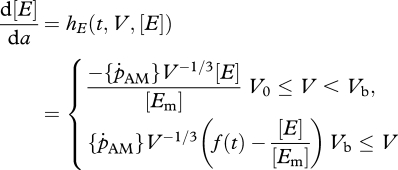
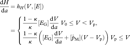
The three life stages, embryo, juvenile and adult, are modelled by continuous-time processes for development, growth and natural mortality. The age, a, dependent DEB model (Kooijman 2000; van der Meer 2006) for the changes of the structure V(a), reserve density [E](a) and cumulative energy allocated to development and reproduction H(a) (in the sequel referred to as maturity; Thieme 1988; van der Meer 2006) reads

2.1a

2.1b

and

2.1c

where the so-called functional response f(t) will be defined later. The initial values for the state of the individual at gametogenesis is indicated by a subscript 0. The initial structural volume of an egg is denoted by V₀ and [E₀] is the reserve density. The initial maturity H₀ equals (1 − κ)/κ[E_G]V₀. Embryos with volume V₀ ≤ V < V_b neither feed nor reproduce. A juvenile is born when the size of the embryo equals V_b. The transition from a juvenile into an adult is at a fixed puberty size V_p. The juveniles with volume V_b ≤ V < V_p consume food but do not reproduce.

Observe that the i-state variable H of equation (2.1c) does not occur on the right-hand side of the equations but it will appear below in the formulation of the jump conditions at the spawning date. We can directly derive for embryos and juveniles V₀ ≤ V ≤ V_p that

2.2

This models the state of maturation. The relationships between the maturity H₀ and H_p and the structural volumes V₀ and V_p read

2.3

We assume starvation when there are not enough reserves to pay the maintenance costs, that is, when κ({ṗ_Am}/[E_m])[E]V^2/3 − [ṗ_M] V < 0. As a consequence, dV/da ≥ 0 and dH/da ≥ 0. Hence, for adults, this means that V ≥ V_p and H ≥ H_p and the i-state variable H models the cumulative energy allocated to reproduction given by H(t) − H_p.

Production of eggs during spawning is modelled by a discrete process occurring (spawning) at a fixed moment of the year. The adults empty their energy reserves allocated for reproduction and the state of maturity becomes H_p again. The number of eggs produced equals the ratio of the amount of energy allocated to reproduction by the adults and the initial energy content of eggs. When the individuals have reached their maximum lifetime, denoted by n ∈ N, they die directly after their last reproduction event. In the next section, reproduction will be modelled at the population level.

(b). Food–population model

Since all individuals reproduce at the same time once per year, it is advantageous to introduce a year-class or a cohort. A new cohort is formed at spawning events, and when they have reached their maximum lifetime, each cohort dies after their last reproduction event. The maximum lifetime in years is therefore also the maximum number of cohorts.

Suppose there is a single founder cohort consisting of identical individuals of the same age. When no reproduction occurs, integration of the following system

2.4a

and

2.4b

gives the dynamic development of the individuals and the cohort as well, where t = a + t₀ with a the age and t₀ the time at gametogenesis of this cohort. The i-state variables, structural volume, energy reserves and maturity represent directly that of the cohort since all individuals are identical and the model is deterministic. N is the number of individuals in the cohort and this number decreases exponentially with mortality rate μ.

During integration, the state-dependent switches defined in equations (2.1) are checked. The jump conditions at the spawning date due to reproduction and death after the last reproduction are derived below.

Owing to the discrete reproduction at one date of the year, the population always consists of just n cohorts. The dynamics of the population are studied in a semi-chemostat environment. Therefore, in the expression for h_E, the first variable X is the time-dependent food concentration in the reactor. The inflowing food concentration is periodical with a period of one year

2.5

The power 4 is used to describe a peaked yearly algal bloom. At t = 0, the inflow of the food supply is maximum. The time at spawning τ is measured relative to this point in time. The maximum of the forcing equals 8.5X̄_in and the minimum 0.5X̄_in.

The periodic forcing and reproduction with the same period of 1 year enables us to introduce a stroboscopic map with a period of 365 days. Generally, the time of reproduction is used as the monitoring date. Then the discrete reproduction and death after the last reproduction take place at the boundary of the interval of 1 year at which the state variables are a smooth function. The discontinuities occur only at the boundary conditions. However, later on, with the study of the evolutionary processes, we will deal with two populations spawning at different times. Therefore, we place the monitoring date at the maximum food inflow rate. As a result, the state variables are only piecewise smooth with cyclic boundary conditions and jumps at the spawning date. Then the time interval of interest is t: 0 ≤ t ≤ 365 with τ the spawning date as an interior point.

We introduce cohorts labelled with a subindex i, that is, i = 1, … , n. At time τ in that interval, the individuals belonging to the first cohort i = 1 have age a = 0 and for 0 ≤ t ≤ 365 their age is a = (t − τ) mod 365. After 1 year, the surviving individuals move to the second cohort i = 2. The actual age of the individuals belonging to cohort i reads a = (t − τ) mod 365 + (i − 1)365. So gametogenesis for the first cohort occurred at t₀ = τ − 365.

The state of the system within each year is described by a finite-dimensional system consisting of one ODE for the food X and for each cohort i, one ODE for each of the three i-state variables: for each cohort, the individual size V_i, reserves [E_i] and maturity H_i, and one ODE for the p-state variable: for each cohort the size N_i. At that event, the population size changes discontinuously whereby the step size depends on the energy stored for reproduction H_i − H_p, where H_p is the maturity threshold.

Then for 0 ≤ t ≤ 365, we have for the system states

2.6a

2.6b

and

2.6c

Here f(X(t)) is the Holling type II functional response:

2.6d

where X_k is the half-saturation constant and we use the fact that embryos do not feed.

Now we formulate the interior jump conditions at the spawning data. The number of eggs produced by the adults form the size of the new cohort

2.7

where [E₀]V₀ is the energy content of one egg and κ_r is the efficiency. The size of cohorts N_i is discontinuous at τ because at that instant for i = 1 a new cohort is formed by the newborns and for i = 2, … , n the individuals become 1 year older, while the cohort of age-class n dies. For the transition of the other cohorts, we have

2.8

whereby cohort n dies at t = τ.

For the i-states, the structural volume and the state of maturity change discontinuously because the energy allocated to reproduction is used for making eggs. So, we have at t = τ

2.9a

2.9b

and

2.9c

for i = 2, … , n.

For the food, we have the continuity condition

2.10

In order to reformulate the problem in terms of the classical nonlinear dynamical system theory, we define the vector of state variables as follows:

2.11

The ODEs for these variables together with the initial conditions for the newborn cohort and reproduction rules, and the cyclic boundary conditions, form a periodically forced system of ODEs. We are looking for periodic solutions of that system and its stability on the ecological time scale. The stroboscopic map is defined as

2.12

where y ∈ N denotes the year at t = 0, that is, at the date where the food inflow is maximum. The fixed point of this nonlinear stroboscopic map Φ gives the periodic solution of the periodically forced system.

Its stability can be studied by an analysis of this stroboscopic map (Kuznetsov 2004). The eigenvalues of the Jacobian matrix of the map Φ evaluated at the fixed point give the local asymptotic behaviour. In our numerical study, the Jacobian matrix is approximated by finite differences. For a stable periodic solution, all eigenvalues must lie inside the unit circle in the complex plane. The periodic solution with the forcing period of 1 year need not be stable in general. To study how the stability depends on the value of a specific parameter, a numerical bifurcation analysis can be performed. Starting from the fixed point solution for the initial parameter value, the bifurcation parameter is varied. During this continuation, the eigenvalues are calculated and they are used to localize critical points where eigenvalues cross the unit circle, that is, where the stability changes. These critical values set the bifurcation points. A period doubling occurs when an eigenvalue equals −1. At a transcritical bifurcation, one eigenvalue equals 1. This happens, for instance, where the population goes extinct. Another possibility is the so-called Neimark–Sacker bifurcation where the magnitude of a pair of complex-conjugated eigenvalues equals 1. Since we are interested in the effects of the time of spawning τ, this parameter is taken as a bifurcation parameter.

(c). Fixed points

At a fixed point, the cyclic boundary conditions read

2.13a

and

2.13b

Where the solution is denoted by a tilde, this indicates periodic dynamics.

Observe that the ODE (2.6b) is de-coupled from the other equations and can be solved directly. When the mortality rate μ is constant, the result is an exponential decay of the number of individuals given by

2.14

Substitution into equation (2.7) gives

2.15

where lim_t↑τ H̃_i(t) is the energy allocated to maturity and reproduction at spawning date. Hence, a necessary condition for a periodic population dynamic is that each individual replaces itself during its lifetime n. This means that the sum of all fertilized eggs produced by one individual at the n spawning events, denoted by R₀, equals 1.

For iteroparous species, we assume that they reproduce possibly every year till the last reproduction before they die. Owing to our starvation condition, we have, as long as the individual stays alive, H ≥ H_p, and therefore it reproduces at the spawning date. Hence, once a cohort has begun to reproduce it will reproduce each subsequent year until the individuals die.

(d). Zero and positive fixed point stability analysis

We first analyse the zero fixed point, where N_i = 0, i = 1, … , n, and thereafter the positive fixed point, where N_i > 0, i = 1, … , n. The obtained results are relevant for the next step, which is the study of the invasion of a mutant population into a resident population. Since Ñ_i = 0, food is not consumed and equation (2.6c) gives the zero fixed-point periodic solution for the food X̃(t) = X_in(t).

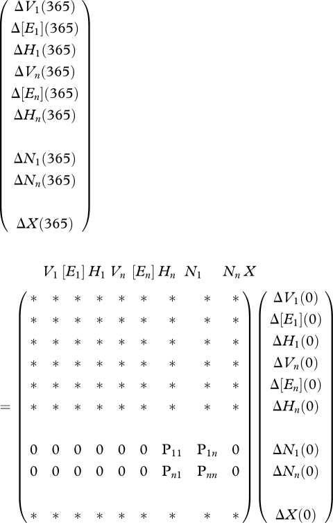
The structure of the Jacobian matrix evaluated at this zero fixed point is indicated below where non-negative elements are denoted by an asterisk.

2.16

The expressions for the elements of the N_i-block matrix follow from

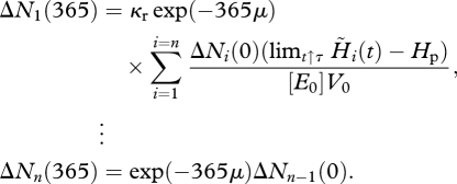The N_i-block matrix P reads

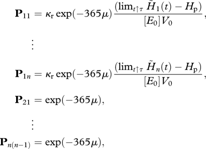and all other elements are zero.

The diagonal block matrix P for the population number variables N_i is decoupled from the i-state variables and food variable system because of the zero elements in the matrix of the two associated rows indicated in equation (2.16). Consequently, the characteristic equation is partitioned and the eigenvalues are those of the two block matrices. Calculations show that for the reference parameter values in table 1, the eigenvalues for the remaining block matrix belonging to the i-state variables and the food variable are inside the unit circle. Some of the eigenvalues are zero and this has to be taken into account in the calculation of the fixed point.

Table 1.

List of symbols. The symbols in the column labelled ‘dimension' stand for: t, time; e, energy; L, length of the organism; l, the length of the reference volume of environment. This reference volume is measured in the arbitrary unit V. The parameter values for an individual life cycle of the Baltic tellin M. balthica are from van der Veer et al. (2006, table 1). The egg energy content is E₀ = [E₀]V₀ = 0.0059 J; hence, assuming that V₀ = 10⁻⁹ cm³, we have [E₀] = 0.59 × 10⁷ J cm⁻³.

symbol	dimension	interpretation	value	unit
a	t	age		days
[E]	eL−3	reserve density		J cm−3
H	e	energy allocated to maturity
		and reproduction		J
N	#l−3	population density		V−1
t	t	time		days
V	L3	structural volume		cm3
X	# l−3	food density		V−1
D	t−1	dilution rate	0.1	d−1
[E0]	—	initial egg reserve density	0.59 × 107	J cm−3
[Em]	eL−3	maximum energy density	2085	J cm−3
[EG]	eL−3	costs of growth	1900	J cm−3
f	—	scaled functional response	—	—
{J̇Xm}	# L−2t−1	maximum area-specific ingestion rate	1	cm−2 d−1
Hp	e	maturity threshold	22.8	J
n	—	maximum lifetime	2	yr
{ṗAm}	eL−2t−1	maximum area-specific assimilation rate	32.9	J cm−2 d−1
[ṗM]	# t−1L−3	volume-specific maintenance rate	24	J cm−3 d−1
V0	L3	initial egg volume	10−9	cm3
Vb	L3	structural volume at birth	10−6	cm3
Vp	L3	structural volume at maturation	0.048	cm3
XK	# l−3	half-saturation coefficient	100	V−1
X̄in	# l−3	proportionality coefficient	1000	V−1
		input food density
κ	—	allocation coefficient	0.8	—
κr	—	efficiency reproduction into eggs	1.18 × 10−5	—
μ	t−1	mortality rate	0.001	d−1
τ	t	spawning date		days

Hence, the stability of the zero fixed-point solution is determined by the n eigenvalues of the diagonal block matrix P. Observe that this matrix is precisely a classical linear Leslie matrix (see Cushing 1998; Caswell 2001). On the first row, the class fertilities and on the sub-diagonal the year-to-year survival probabilities are shown. The eigenvalues and eigenvectors of this non-negative matrix are described by the Perron–Frobenius theorem (Caswell 2001, p. 83). Furthermore, it allows for the use of net reproductive rate denoted by R₀ for the evaluation of the stability (Caswell 2001, p. 83): R₀ > 1 unstability and R₀ < 1 stability. Here we use the dominant eigenvalue of the block matrix P. For the reference parameter values, one of the real eigenvalues is inside the unit circle but the other is outside and therefore the zero fixed-point solution is unstable. This finalizes the analysis of the zero fixed point where N_i = 0, i = 1, … , n.

Besides this zero fixed point, there can be positive solutions where N_i > 0, i = 1, … , n. The analysis of these positive solutions is straightforward since no degeneracies nor partitions of the Jacobian matrix occur. Therefore, the eigenvalues of the Jacobian matrix directly dictate the stability properties.

3. Evolutionary model formulation

We will study the evolutionary development of the population in the reactor using the AD approach. It is assumed that the ecological time scale (here a few years) is much faster than the evolutionary time scale (several generations). The ecological time scale is set by the rate of convergence to the stable periodic solution. The evolutionary time scale is set by the rate of change of the trait parameter, the low mutation rate. The trait is the timing of the reproduction τ. Hence, individuals from the resident and mutant population have the same physiological parameter values except for the timing of reproduction τ. Time-scale separation gives that in studying the dynamics of the trait the population dynamic is at a steady state, that is, at a stable fixed point of the stroboscopic map, equation (2.12).

In order to study the effects of a mutational step, we introduce, besides the steady-state resident population with trait value τ = τ_r, a mutant population with a slightly different trait value τ = τ_m. As a result, the dynamics of the extended dynamical system now consisting of two populations is studied. In a similar way as for a one population system, a stroboscopic map can be formulated. Both populations compete for the same food X, so the ODE for the food reads

3.1

where the additional subscript denotes the resident, r, or mutant, m, population.

In summary, the governing equations for the resident and mutant population in the chemostat reactor are formed by equations (2.12) whereby the vector of state the variables reads

3.2

where for all i-states and p-states, v ∈ {V,[E],H, N}, and both populations, P ∈ {r, m}

3.3

To study invasion of the resident population by a mutant population, we consider the stability of the fixed point whereby N_i,r > 0 and the mutant is absent, N_i,m = 0, i = 1, … , n.

4. Bifurcation analysis technique

For the periodically forced system studied here, we use the bifurcation analysis approach to calculate the PIP and MIP. Regions of co-existence of the resident and mutant populations are bounded by transcritical bifurcations of the stroboscopic map (Kooi & Troost 2006; Troost et al. 2007, 2008). At these curves, the system consisting of the resident and mutant populations together with the ambient food is structurally unstable with the leading eigenvalue equal to 1, whereby one population (here we assume first the mutant population) is absent and its invasion rate is zero. These curves mark the regions of co-existence.

Applying bifurcation theory means that the ESS is fixed by a point τ_m = τ_r where two transcritical bifurcation curves (one where the resident population is absent and the other where the mutant population is absent) intersect. Observe that at this point there is no unique solution because the two populations are identical and therefore only the sum of the numbers of individuals that make up the populations is fixed. The type of ESS can be found by performing a one-parameter bifurcation analysis where τ_r = τ_m + ɛ, where ɛ is small.

As for the zero solution of the one-population map, it is possible to derive analytically some general results before performing a numerical bifurcation analysis whereby all parameters need to possess a value, except the free bifurcation parameter (here the trait). The situation is similar to that discussed above for the zero fixed-point solution whereby the number density of the population was zero, that is, N_i = 0 in the mutant population. The food density X(t) is now not equal to the input function X_in(t) but is set by the resident population. Nevertheless, there is a partitioning of the Jacobian matrix, here for the mutant i-state variables V_i,m, [E_i,m], H_i,m and the mutant p-state N_i,m, i = 1, … , n and a coupled set consisting of the food density X and the complete resident population i-state and p-state variables. The block matrix related to the latter set of variables equals the Jacobian matrix of the dynamical system with the resident population alone in the chemostat. Since the mutant population has number density zero, there is effectively no competition and this gives the decoupling. We assume that the invaded resident population possesses a stable fixed point.

Consequently, also in this case, we need to evaluate only the stability of the n-dimensional system for N_i,m, i = 1, … , n. Since the periodic solution of the resident population system with spawning date τ_r is stable, the invasion fitness (Metz et al. 1992) is just the dominant eigenvalue of the Jacobian block matrix P for the mutant population with spawning date τ_m evaluated at N_i,m = 0, i = 1, … , n. When this dominant eigenvalue is outside the unit circle, the mutant can invade; otherwise it cannot.

Alternatively, using the expression for R₀ in equation (2.15), we can obtain the following invasion fitness s = ln R₀ for the mutant population with spawning date τ_m

4.1

Here H_i,m(t) is calculated using the food dynamics set by the resident population.

5. Case study

Many students of marine invertebrates have considered the fitness consequences of the timing of reproduction only in terms of the short-term prospects of the offspring (Thorson 1966). For example, it has recently been argued that spawning of the marine bivalve M. balthica, which seems to be triggered by a temperature threshold, has shifted forward within the season as a result of global change (Philippart et al. 2003). This may have caused a temporal mismatch with the onset of the spring bloom which is believed to be of vital importance for the early larvae. Generally speaking, it is, however, not immediately obvious why emphasis should be put on the earliest life phase of the offspring. Adults themselves may profit from the food peak and by these means increase the total reproductive output. It might also be more profitable for the young to experience the food peak at a later stage and a larger size (Schultz et al. 1991). The debate on whether growth and development of invertebrate larvae are indeed food limited under natural conditions has not been settled yet (Strathmann 1996).

In this section, we present results of our analysis for the bivalve M. balthica. Our exploration on the optimal time of spawning for this bivalve may contribute to the discussion on the importance of the food conditions during the earliest life larval phase of marine invertebrates. The parameter values of the DEB model for M. balthica were estimated in van der Veer et al. (2006) and are given in table 1. Macoma balthica lives buried in sandy sea beds of the coastal zones of the Northern Atlantic. Along the European coast, M. balthica occurs from the White Sea at 70° N to the Gironde estuary at 45° N. In the Dutch Wadden Sea where M. balthica is a dominant species, it can be found from the upper regions of the intertidal to the outer parts of the tidal inlets and into the coastal zone. It feeds only on algae. In the Dutch Wadden Sea, M. balthica spawns in April (Philippart et al. 2003), while the chlorophyll levels, which are indicative of algal abundance, peak in May (Philippart et al. 2003).

We also studied the impact of a number of parameters related to the interaction of the population with the environment while keeping all DEB for the individuals the same as in table 1. We studied the temperature effects affecting the physiological rates using the Arrhenius relationship whereby the ambient temperature (and therefore also the internal temperature of most marine organisms) fluctuates annually. The parameter values in the periodic forcing function for the food given in equation (2.5) also varied. Furthermore, we increased the maximum lifetime from 2 to 5. The results are not discussed here.

(a). Bifurcation analysis results

We start with the analysis of the ecological model in which the trait, the time of spawning τ, is fixed for the resident population.

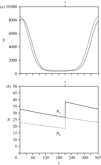
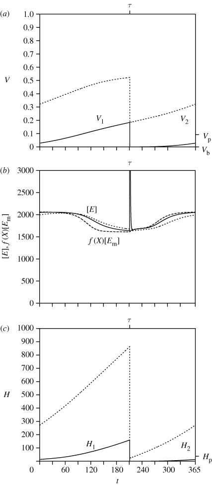
For the parameter values given in table 1, the zero solution where N_i = 0, for i = 1, 2, is unstable. The dominant eigenvalue of the 2 × 2, Jacobian block matrix for the p-state variables N_i, i = 1, 2, is larger than 1 and the other eigenvalues are inside the unit cycle. The positive solution is, however, stable for the parameter values given in table 1. This stable periodic solution of the resident population is shown in figures 1 and 2 for τ = 211 days. From the analysis below, we know that this trait value belongs to an ESS. Figure 1a gives the annual cycle of the inflowing food concentration X_in(t) and the ambient food concentration X(t). The food concentration increases at spawning. This is because the newly laid eggs do not feed while the adults in the second year-class cohort died. In general, the difference between X_in(t) and X(t) is due to feeding of the population which causes some delay, well known for predator–prey interactions.

Figure 1.

(a) Food concentration X_in supplied, ambient food concentration X. (b) Population densities of the cohorts N_i, i = 1, 2. The two p-state variables are plotted as a function of the time t where τ = 211 days.

Figure 2.

(a) Individual biovolumes of the cohorts V_i, i = 1, 2. (b) Energy reserves of the cohorts [E_i], i = 1, 2 and the expression f(t)[E_m]. (c) Maturity: cumulative energy allocated to development (embryos and juveniles) or reproduction (adults) of the cohorts H_i, i = 1, 2. The three i-state variables are plotted as a function of the time t where τ = 211 days.

The number of individuals in each cohort N_i(t), i = 1, 2, is depicted in figure 1b. These numbers are continuously decreasing due to mortality and discontinuously due to the disappearance of the second year-class cohort after their final spawning event; only at spawning is there an increase due to egg production of the first-year cohort. The transition from each year-class cohort to the next year-class is continuous; all individuals move to the next class.

In figure 2, the changes of the i-state of the individuals in their first- and second-year classes are depicted, where age is related to time of year by a = ((t − τ) mod 365) + (i − 1)365, where i is the year class. In figure 2a, the size v of the eggs is small at spawning. They hedge and become juvenile at V_i = V_b, and become mature at V_i = V_p, i = 1, 2. Observe that there is always growth; the individuals do not shrink, not even during time periods where the food density is low. Figure 2b shows the annual changes in the energy allocation to the reserve buffer [E_i](t) together with the expression f(t)[E_m] (see equation (2.1b)). In figure 2c, the energy allocation to development and the reproduction H_i(t) is shown.

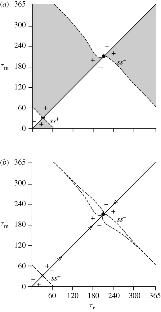
The PIP and MIP shown in figure 3 summarize the evolutionary results. Figure 3a is the PIP. In the grey regions, the mutant is able to invade the resident population, that is, the mutants fitness is positive. At the interior boundaries, the invasion fitness is zero. The point on the principle diagonal where the fitness gradient is zero is an ESS. The MIP (figure 3b) is obtained as the superposition of the PIP and its mirror image along the principle diagonal (Geritz et al. 1998). On the right side of the point ss⁻, there is a plus below the diagonal and a minus above the diagonal. That is, the local fitness gradient from above points towards ss⁻. On the left side of the point ss⁻, there is a minus below the diagonal and a plus above the diagonal. Hence, the local fitness gradient from below also points towards ss⁻. This description is that of the AD framework.

Figure 3.

(a) PIP. In the grey regions, the mutant may invade and replace the resident, and in the white regions, it cannot invade. There is a stable singular point ss⁻ and an unstable singular point ss⁺. (b) MIP. The ‘ + ’-mutant may invade and replace the resident and the ‘ − ’-mutant cannot invade. The dashed curves are the transcritical bifurcation curves. The arrows indicate the direction of the evolution.

Now we give a description of the results of applying the bifurcation analysis approach. Here we only refer to the MIP (figure 3b). In this diagram, the transcritical bifurcation curves are drawn. There are two types of curves. At one curve, the size of the mutant population is zero, and at the other type of curve, the size of the resident population is zero. These curves mark the trait values where the invasion rate of the zero-size population is zero. There is an ESS at the intersection point on the diagonal where these curves meet. There are two ESSs: point ss⁻ at τ_r = 211 days and point ss⁺ at τ_r = 31.2 days.

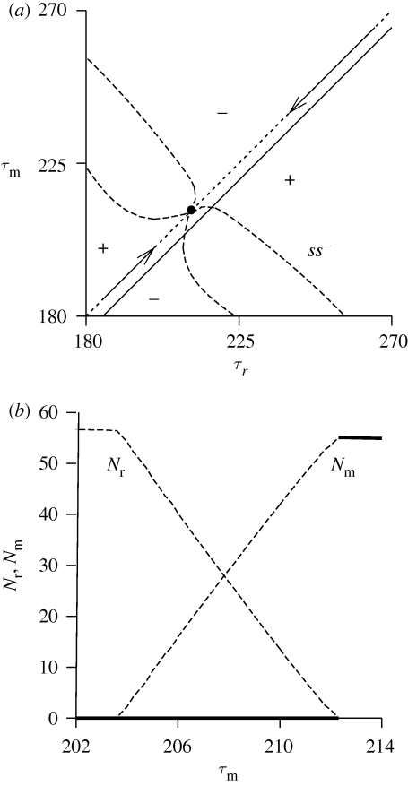
The transcritical curves close to the point ss⁻ enclose a region where the two populations can co-exist (see MIP; figure 3b). However, this interior point is unstable (the leading eigenvalue of the Jacobian matrix evaluated at points in this region is outside the unit cycle). Figure 4b is a one-parameter diagram showing the population size N_r = ∑_i=1² N_r,i of the resident population and N_m = ∑_i=1² N_m,i of the mutant population as a function of the trait τ_m, where τ_r = τ_m + 5. This line is also drawn in figure 4a, which is a detail of figure 3b. The interior equilibrium is always unstable (at the ecological time scale) and therefore branching does not occur and point ss⁻ is a stable ESS. The diagram shows that there is no mutual invasibility. The zero fixed point is stable below the right (catastrophic) transcritical bifurcation point and the positive fixed point is stable above this bifurcation point.

Figure 4.

(a) Detail of figure 3b around the point ss⁻. The drawn line is τ_r = τ_m + 5. (b) Population densities of resident (N_r = ∑_i=1² N_r,i) and mutant (N_m = ∑_i=1² N_m,i) populations as a function of the trait τ_m where τ_r = τ_m + 5. Solid lines denote the stable fixed points and dashed lines the unstable fixed points.

In a similar way, we find that the local fitness gradient points, in both directions, away from ss⁺. This point forms a separatrix. Starting with a higher resident trait values, mutational steps will lead to an increase in the trait towards point ss⁻. On the other hand, starting with a smaller trait value, mutational steps lead to a decrease towards point ss⁻, where we use the fact that the PIP is cyclic for τ = 0 and τ = 365.

For points that are more distant from the points ss⁻ and ss⁺ in figure 3b, the region of co-existence becomes very small and both curves are indistinguishable. Because the PIP is cyclic with a period of 1 year, the transcritical bifurcation curves connect points ss⁻ and ss⁺. When the two curves coincide, the dynamics are the same as on the diagonal; at one side one population wins while at the other side the other wins.

6. Discussion

The main aim of this paper is to study the evolutionary dynamics of the timing of spawning within the year. The work here differs from that of Davydova (2004) using semelparous species (n = 1) in that the population is iteroparous, that is, the individuals reproduce annually and die immediately after the last reproductive event (n ≥ 2).

In the AD theory literature, the PIP and MIP are constructed by calculation of the zero invasion fitness curves (Metz et al. 1996; Geritz et al. 1998). Thereafter, the shape of these curves directly fixes the ESS points and their evolutionary stability (Geritz et al. 1998). Eight different types of singular strategies are distinguished based on the second derivatives of the invasion fitness evaluated at the point. The region of invasion in the PIP (figure 3a) close to the point ss⁻ at τ_r = 211 days is the same as in Geritz et al. (1998, fig. 2, case (e)): it is ESS stable and convergence stable. The local fitness gradient points towards this point. For point ss⁺ at τ_r = 31.2 days, the region of invasion is the same as that in Geritz et al. (1998, fig. 2 case (h): it is ESS unstable and convergence unstable.

In the AD approach, a mutational step is divided into two steps. First a stable resident population is invaded by the mutant population, second the mutant population replaces the resident population and this means that the new resident population is also stable. In bifurcation terms, these two steps mean that starting from a stable resident population, first the resident–mutant system with zero mutant population size but with a sightly different trait value than the resident population is unstable. Second, the resident population goes extinct and the mutant population grows and reaches a stable fixed point. In our approach, the stability of the new resident population is checked when the next mutational step is analysed.

In a bifurcation analysis context, the zero mutant invasion fitness curve is precisely the transcritical bifurcation curve for the two-population system in the two-dimensional trait space, where the trait of the resident and mutant populations are the bifurcation parameters. Generally, this is achieved by the calculation of the so-called test functions (see Kuznetsov 2004) or by the calculation of the eigenvalues of the Jacobian matrix. It is also possible to use the zero-invasion fitness curve defined in equation (4.1). This simplifies the numerical calculations, for there is no need to calculate the Jacobian matrix evaluated at the fixed point and its eigenvalues. However, using the invasion fitness as a test function gives no guaranty that the invaded resident population is stable and, furthermore, no direct information about whether invasion leads to replacement or co-existence.

The bifurcation diagram figure 3b is an alternative to the PIP (figure 3a). The advantage of a bifurcation analysis is that it is also applicable when no simple expression for the invasion fitness is available. Furthermore, because all types of bifurcations are calculated as part of the analysis of the competitive two-population system, the requirements (for instance, the existence of a positive stably resident population) that justify the application of the AD approach are checked. Observe that in the bifurcation analysis approach, we adhere strictly to the time-scale separation of the ecological and evolutionary time scales. After a successful invasion of the mutant, it replaces the resident population. This means that the temporal change of the trait variables at the evolutionary time scale, described by the canonical equation (Dieckmann & Law 1996), is not studied: only the calculation and evaluation of the stability of the evolutionary endpoints. In Dercole & Rinaldi (2008), the dynamics of the canonical equation is studied in great detail using the bifurcation analysis technique.

In de Roos et al. (2006), a size-structured population–nutrient model is used to study the evolutionary changes in fish individual life history and stock properties. In that article, many elements of the AD approach are adopted. The invasion fitness is computed by two-population competition simulations. This approach is more universal and can be used for a wide range of population models and also when the ecological and evolutionary time scales are not separated (see also Troost et al. 2008). However, the accuracy of the simulation can be problematic and the calculations are much more time-consuming.

Although the results obtained for the bivalve M. balthica are preliminary, it is tempting to compare them with field data. From figure 3, we learn that there are two ESS values, one is an evolutionary attractor and the other is an evolutionary repeller. At the attracting singular strategy, the species spawns about 150 days before the maximum food inflow (algal bloom). This date is far away from what has been observed in the field, where spawning occurs only one month before the algal bloom (Philippart et al. 2003). At present, knowledge at the individual level is much more extensive than what we know at the population level, including the description of food and predation dynamics. DEB parameter values, for example, are relatively well known (van der Veer et al. 2006). Hence, there is a need for more data at the population level. Nevertheless, we can conclude that the accepted hypothesis that the seasonal timing of spawning in marine invertebrates is a response to seasonal fluctuations in food levels was not confirmed by our model analysis. It might be that, besides the dynamics of the food, the seasonal fluctuations in predation pressure are important.

In conclusion, bifurcation analysis provides an integrated approach for modelling and analysis of ecological and evolutionary processes at both individual and population levels of organization. In the future, the technique developed here will be used to study the evolution of reproductive strategies such as the timing of spawning of marine invertebrates or vertebrates that spawn within small time windows periodically (Olive et al. 1997; Watson et al. 2000; Reitzel et al. 2004; Varpe et al. 2007, 2009).

References

- Allgower E. L., Georg K.1990Numerical continuation methods. An introduction. Springer Series in Computational Mathematics, vol. 13 Berlin, Germany: Springer-Verlag [Google Scholar]
- Bazykin A. D.1998Nonlinear dynamics of interacting populations. Singapore, Singapore: World Scientific [Google Scholar]
- Caswell H.2001Matrix population models, construction, analysis, and interpretation. Sunderland, MA: Sinauer Associates Inc [Google Scholar]
- Cushing J. M.1998An introduction to structured population dynamics, vol. 71 Philadelphia, PA: Society for Industrial and Applied Mathematics [Google Scholar]
- Davydova N. V.2004Old and young. Can they coexist? PhD thesis, Utrecht University, The Netherlands [Google Scholar]
- de Roos A. M.1997A gentle introduction to physiologically structured population models. In Structured-population models in marine, terrestrial, and freshwater systems (eds Tuljapurkar S., Caswell H.), pp. 119–204 New York, NY: Chapman & Hall [Google Scholar]
- de Roos A. M., Boukal D. S., Persson L.2006Evolutionary regime shifts in age and size at maturation of exploited fish stocks. Proc. R. Soc. B 273, 1873–1880 (doi:10.1098/rspb.2006.3518) [DOI] [PMC free article] [PubMed] [Google Scholar]
- Dercole F., Rinaldi S.2008Analysis of evolutionary processes: the adaptive dynamics approach and its applications. Princeton, NJ: Princeton University Press [Google Scholar]
- Dhooge A., Govaerts W., Kuznetsov Yu. A.2003Matcont: a MATLAB package for numerical bifurcation analysis of ODEs. ACM Trans. Math. Softw. 29, 141–164 (doi:10.1145/779359.779362) [Google Scholar]
- Dieckmann U., Law R.1996The dynamical theory of coevolution: a derivation from stochastic ecological processes. J. Math. Biol. 34, 579–612 (doi:10.1007/BF02409751) [DOI] [PubMed] [Google Scholar]
- Diekmann O., Gyllenberg M., Metz J. A. J., Thieme H. R.1998On the formulation and analysis of general deterministic structured population models. I. Linear theory. J. Math. Biol. 36, 349–388 (doi:10.1007/s002850050104) [DOI] [PubMed] [Google Scholar]
- Diekmann O., Gyllenberg M., Huang H., Kirkilionis M., Metz J. A. J., Thieme H. R.2001On the formulation and analysis of general deterministic structured population models. II. Nonlinear theory. J. Math. Biol. 43, 157–189 (doi:10.1007/s002850170002) [DOI] [PubMed] [Google Scholar]
- Doedel E. J., Oldeman B.2009Auto 07p: continuation and bifurcation software for ordinary differential equations. Technical report, Concordia University, Montreal, Canada [Google Scholar]
- Geritz S. A. H., Kisdi É., Meszéna G., Metz J. A. J.1998Evolutionarily singular strategies and the adaptive growth and branching of the evolutionary tree. Evol. Ecol. 12, 35–57 (doi:10.1023/A:1006554906681) [Google Scholar]
- Geritz S. A. H., van der Meijden E., Metz J. A. J.1999Evolutionary dynamics of seed size and seedling competitive ability. Theor. Popul. Biol. 55, 324–343 (doi:10.1006/tpbi.1998.1409) [DOI] [PubMed] [Google Scholar]
- Guckenheimer J., Holmes P.1985Nonlinear oscillations, dynamical systems and bifurcations of vector fields, applied mathematical sciences, vol. 42, 2nd edn. New York, NY: Springer-Verlag [Google Scholar]
- Kooi B. W.2003Numerical bifurcation analysis of ecosystems in a spatially homogeneous environment. Acta Biotheor. 51, 189–222 (doi:10.1023/A:1025146207201) [DOI] [PubMed] [Google Scholar]
- Kooi B. W., Troost T. A.2006Advantages of storage in a fluctuating environment. Theor. Popul. Biol. 70, 527–541 (doi:10.1016/j.tpb.2006.07.005) [DOI] [PubMed] [Google Scholar]
- Kooijman S. A. L. M.2000Dynamic energy and mass budgets in biological systems. Cambridge, UK: Cambridge University Press [Google Scholar]
- Kozlowski J.1996Optimal allocation of resources explains interspecific life-history patterns in animals with indeterminate growth. Phil. Trans. R. Soc. Lond. B 263, 559–566 (doi:10.1098/rstb.1996.0084) [Google Scholar]
- Kuznetsov Y. A.2004Elements of applied bifurcation theory. Applied Mathematical Sciences, vol. 112, 3rd edn. New York, NY: Springer-Verlag [Google Scholar]
- McNamara J. M., Houston A. I.2008Introduction. Adaptation to the annual cycle. Phil. Trans. R. Soc. B 363, 209–210 (doi:10.1098/rstb.2007.2192) [DOI] [PMC free article] [PubMed] [Google Scholar]
- Metz J. A. J., Diekmann O.1986The dynamics of physiologically structured populations. Lecture Notes in Biomathematics, vol. 68 Berlin, Germany: Springer-Verlag [Google Scholar]
- Metz J. A. J., Geritz S. A. H., Nisbet R. M.1992How should we define ‘fitness’ for general ecological scenarios? Trends Ecol. Evol. 7, 198–202 (doi:10.1016/0169-5347(92)90073-K) [DOI] [PubMed] [Google Scholar]
- Metz J. A. J., Geritz S. A. H., Meszéna G., Jacobs F. J. A., van Heerwaarden J. S.1996Adaptive dynamics, a geometrical study of the consequences of nearly faithful reproduction. In Stochastic and spatial structures of dynamical systems (eds van Strien S. J., Verduyn Lunel S. M.), pp. 183–231 Amsterdam, The Netherlands: North-Holland [Google Scholar]
- Olive P. J. W., Porter J. S., Sandeman N. J., Wright N. H., Bentley M. G.1997Variable spawning success of Nephtys hombergi (Annelida: Polychaeta) in response to environmental variation a life history homeostasis? J. Exp. Mar. Biol. Ecol. 215, 247–268 (doi:10.1016/S0022-0981(97)00047-6) [Google Scholar]
- Parker T. S., Chua L. O.1989Practical numerical algorithms for chaotic systems. Berlin, Germany: Springer-Verlag [Google Scholar]
- Philippart C. J. M., van Aken H. M., Beukema J. J., Bos O. G., Cadee G. C., Dekker R.2003Climate-related changes in recruitment of the bivalve Macoma balthica. Limnol. Oceanogr. 48, 2171–2185 (doi:10.4319/lo.2003.48.6.2171) [Google Scholar]
- Reitzel A. M., Miner B. G., McEdward L. R.2004Relationships between spawning date and larval development time for benthic marine invertebrates: a modeling approach. Mar. Ecol. Prog. Ser. 280, 13–23 (doi:10.3354/meps280013) [Google Scholar]
- Roff D. A.2002Life history evolution. Sunderland, MA: Sinauer Associates [Google Scholar]
- Schultz E. T., Clifton L. M., Warner R. R.1991Energetic constraints and size-based tactics: the adaptive significance of breeding-schedule variation in a marine fish (Embiotocidae: Micrometrus minimus). Am. Nat. 138, 1408–1430 (doi:10.1086/285294) [Google Scholar]
- Strathmann R. R.1996Are planktonic larvae of marine benthic invertebrates too scarce to compete within species? Oceanol. Acta 19, 399–407 [Google Scholar]
- Thieme H. R.1988Well-posedness of physiologically structured population models for Daphnia magna. J. Math. Biol. 26, 299–317 (doi:10.1007/BF00277393) [Google Scholar]
- Thorson G.1966Some factors influencing the recruitment and establishment of marine benthic communities. Nether. J. Sea Res. 3, 267–293 (doi:10.1016/0077-7579(66)90015-9) [Google Scholar]
- Troost T. A., Kooi B. W., Kooijman S. A. L. M.2007Bifurcation analysis of ecological and evolutionary processes in ecosystems. Ecol. Model. 204, 253–268 (doi:10.1016/j.ecolmodel.2007.01.007) [Google Scholar]
- Troost T. A., Kooi B. W., Dieckmann U.2008Joint evolution of predator body size and prey-size preference. Evol. Ecol. 22, 771–799 [Google Scholar]
- van der Meer J.2006An introduction to dynamic energy budget (DEB) models with special emphasis on parameter estimation. J. Sea Res. 56, 85–102 (doi:10.1016/j.seares.2006.03.001) [Google Scholar]
- van der Veer H. W., Cardoso J. F. M. F., van der Meer J.2006The estimation of DEB parameters for various northeast atlantic bivalve species. J. Sea Res. 56, 107–124 (doi:10.1016/j.seares.2006.03.005) [Google Scholar]
- Varpe Ø., Jorgensen C., Tarling G. A., Fiksen Ø.2007Early is better: seasonal egg fitness and timing of reproduction in a zooplankton life-history model. Oikos 116, 1331–1342 (doi:10.1111/j.0030-1299.2007.15893.x) [Google Scholar]
- Varpe Ø., Jorgensen C., Tarling G. A., Fiksen Ø.2009The adaptive value of energy storage and capital breeding in seasonal environments. Oikos 118, 363–370 (doi:10.1111/j.1600-0706.2008.17036.x) [Google Scholar]
- Watson G. J., Williams M. E., Bentley M. G.2000Can synchronous spawning be predicted from environmental parameters? A case study of the lugworm Arenicola marina. Mar. Biol. 136, 1003–1017 (doi:10.1007/s002270000283) [Google Scholar]
- Wiggins S.1990Introduction to applied nonlinear dynamical systems and chaos. Texts in Applied Mathematics, vol. 2 New York, NY: Springer-Verlag [Google Scholar]