Corrections to linear methods for diffuse optical tomography using approximation error modelling

Abstract

Linear reconstruction methods in diffuse optical tomography have been found to produce reasonable good images in cases in which the variation in optical properties within the medium is relatively small and a reference measurement with known background optical properties is available. In this paper we examine the correction of errors when using a first order Born approximation with an infinite space Green’s function model as the basis for linear reconstruction in diffuse optical tomography, when real data is generated on a finite domain with possibly unknown background optical properties. We consider the relationship between conventional reference measurement correction and approximation error modelling in reconstruction. It is shown that, using the approximation error modelling, linear reconstruction method can be used to produce good quality images also in situations in which the background optical properties are not known and a reference is not available.

1. Introduction

In diffuse optical tomography (DOT), the goal is to produce quantitative images of the optical properties of an unknown medium based on near-infrared light transport measurements made on the surface of the object [1,4,7]. Since the photons travel randomly inside the medium, image reconstruction is a highly ill-posed problem and needs to be approached within the framework of inverse problems. In these methods, light propagation is modelled using the radiative transport equation (RTE) or its approximations [1,5,13]. In turbid media, the most commonly applied model is the diffusion approximation (DA) to the RTE. The accurate modelling of light transport and usage of sophisticated image reconstruction methods have enabled production of good quality optical images which strongly supports the view that DOT is one of the most promising new medical imaging modalities. However, DOT still needs further development, and, in particular, accurate and fast image reconstruction methods that could be used simultaneously with measurements and in online monitoring need to be developed.

The existing approaches in DOT can be classified into those based on inverse scattering theory (IST) and analytical (Green’s function) solutions to the light propagation model [21], and those based on data fitting using optimisation techniques and numerical solutions to the underlying partial differential equations [1], also known as the parameter identification method (PIM). Although these two methods are thought of as quite different, we will show in this paper that both can be put into a common framework when we consider a Bayesian approach to analysing the underlying model errors.

In both the IST and PIM frameworks, either a linear or a non-linear approach to the inverse problem can be developed, and the central computational requirement for the forward problem is to construct a suitable model for the sources and detectors which can be used to match the experimental data taken on the turbid medium’s surface. However, it is generally true that the difficulty of producing highly accurate computational models can be significant, and is counterintuitive in regard to the inherently poor resolution of DOT. In practice, the models used are only approximate and have to be ‘corrected’ (or to use a more principled term ‘calibrated’) to actually work in practice. Usually, the correction is achieved using reference measurements.

Linearisation of the inverse problem is explicit in the IST approach and in iterative Newton type algorithms in the PIM approach. In the former technique, the linearisation is built from analytic Green’s functions which solve the DA in predetermined domain such as an infinite space [2, 20]. These linear methods are limited by the fact that they cannot predict large changes in the optical parameters and that they assume the background optical properties to be known [6]. However, such methods have been found to produce good quality images in situations in which these limitations are fulfilled and a reference measurement from known background medium is available [15]. The linearisation error in an another diffuse imaging modality, electrical impedance tomography, has been addressed in [23].

In this paper, we use the approximation error modelling theory to explain the connection between the IST and PIM approaches. The approximation error approach for the treatment of modelling errors was introduced in [11, 12]. The method has been applied in DOT in compensating modelling errors due to discretisation, domain mismodelling and in compensating modelling errors between the RTE and the DA [3, 8, 14, 24]. Outside optical imaging, the approximation error approach has been utilised in electrical impedance tomography [11, 16–19] and it has been extended to time-dependent inverse problems [9, 10]. In this paper, we develop an approach in which the approximation error approach is used to correct the linear reconstruction method in DOT. In this approach, a reference measurement is not needed and the background optical properties do not need to be known but a model for the uncertainty of the background coefficients is needed.

The rest of the paper is organised as follows. In Section 2, linear reconstruction methods in DOT are reviewed. In Section 3, the approximation error approach is described and its relation to reference measurement approach is explained. In Section 4, simulation results are shown and in Section 5 conclusions are given.

2. Deterministic model based reconstruction and correction methods

2.1. Definitions.

We are considering the fitting of a model

$$y=A\left(x\right)+e,A:𝕏\to {ℝ}^m$$ (1)

where y ∈ ℝ^m is discrete data, x ∈ 𝕏 is a function in some space 𝕏 representing the absorption and scattering images, and e denotes the noise which is usually modelled to be Gaussian distributed e ~ �©(0,Γ_e) with zero mean and covariance Γ_e ∈ ℝ^m×m. In the ‘true’ physical problem we assume 𝕏 = L^∞(�©) but in a practical implementation the solution and forward mapping are represented in discrete vector spaces

$$x\mapsto x_h\in {ℝ}^n,A\mapsto A_h$$ (2)

where A_h : ℝⁿ → ℝ^m is a linear or non-linear operator.

Throughout this paper, within both the IST and PIM frameworks we assume that the light propagation model is the diffusion approximation

$$\left(-\nabla ·D\nabla +{\mu }_a+\frac{i\omega }{c}\right)\Phi =0,\mathrm{in}\mathrm{�\copyright }$$ (3)

$$\Phi +2\mathit{\zeta D}\frac{\partial \Phi }{\partial \nu }=J^{-},\mathrm{on}\partial \mathrm{�\copyright }$$ (4)

which is denoted as

$$𝓛\left(x\right)\Phi =J^{-}.$$ (5)

In Eqs. (3)–(5), D = (3(μ_a + μ_s^′))^-1 is the diffusion coefficient, μ_s^′ is the reduced scattering coefficient, μ_a is the absorption coefficient, Φ is the photon density, J^- is prescribed input source function, i is the imaginary unit, c is the speed of light in the medium and ω is the angular modulation frequency of the input signal. Furthermore, in this paper we use the following notations

background optical parameters:	x0 = (μa,0,μs,0′)T
perturbed optical parameters:	x=(μa,μs′)T=x0 + δx
estimated optical parameters:	x̂
measured data :	gobs
reference data :	gref
modelled data :	y
modelled reference data :	y0
discretized (incorrect) background optical parameters:	xh,0
discretized (incorrect) optical parameters:	xh = xh,0 + δxh
exact model for the forward operator in domain �©:	A
approximate model in (incorrect) domain �©̃:	Ah
augmented model :	Ãh
Jacobian:	J
modelling error:	ε

2.2. Linear reconstruction model within inverse scattering theory.

In the IST approach we represent the operator A in Eq. (1) as the measurement of the Green’s function

$$A\left(x\right)=\mathrm{𝓜𝓖}\left(x\right)J^{-}$$ (6)

where 𝓖(x) is the Green’s operator, parameterised by x, that solves for the internal field Φ given the source function and the light propagation model (5) and ℳ is the measurement of Φ at the boundary of the domain �©. In practice, measurements are needed for multiple input sources functions {J₁^-, J₂^-,…} where the functions {J_i^-} form a basis for general functions on the boundary ∂�©, leading to a vector form for the forward model

$$A\left(x\right)=\left(\begin{array}{c}{𝓜}_1𝓖\left(x\right)J_1^{-}\\ {𝓜}_2𝓖\left(x\right)J_2^{-}\\ ⋮\\ {𝓜}_S𝓖\left(x\right)J_S^{-}\end{array}\right).$$ (7)

Under this notation, given a reference state x₀, a series solution for a perturbed state x₀ + δx is given by

$$A\left(x_0+\mathit{\delta x}\right)=𝓜{\left[𝓘-𝓖\left(x_0\right)𝓥\left(\mathit{\delta x}\right)\right]}^{-1}𝓖\left(x_0\right)$$
$$=A\left(x_0\right)+𝓜\left[𝓖\left(x_0\right)𝓥\left(\mathit{\delta x}\right)+{\left(𝓖\left(x_0\right)𝓥\left(\mathit{\delta x}\right)\right)}^2+\dots \right]𝓖\left(x_0\right),$$ (8)

where 𝓘 is an identity operator and 𝒱(δx) is a potential operator determined by the perturbation. Eq. (8) is a general Born series for diffuse photon density waves.

Linear inversion methods in DOT based on the series Eq. (8) consider only the first term in the series and make the approximation

$$A\left(x_0+\mathit{\delta x}\right)=A\left(x_0\right)+\mathrm{�\copyright }\left(x_0\right)\mathit{\delta x},$$ (9)

where the Jacobian �©(x₀) is the discrete representation of the Fr�©chet derivative of the nonlinear mapping A(x), and seek to invert the linear expression

$$g^{\mathrm{obs}}-y_0=\mathrm{�\copyright }\left(x_0\right)\mathit{\delta x},$$ (10)

where g^obs are measurements and y₀ = A(x₀) is assumed to be an accurate prediction of the measurements that would correspond to the reference state x₀.

It is natural to consider both the accuracy of the prediction of y₀ at measurement position r_m due to source located r_s as well as the accuracy of representation of the linearisation �©(x₀) which both depend on the accuracy of the Green’s functions

$$y_0|r_m=𝓜{\int }_{\mathrm{�\copyright }}G(r_m,r_s;x_0)J^{-}\left(r_s\right)d{r}_s$$ (11)

$$\left(y-y_0\right)|r_m=𝓜{\int }_{\mathrm{�\copyright }}G(r_m,r\prime ;x_0)𝓥\left(\mathit{\delta x}\right)G\left(r\prime ,r_s;x_0\right)J^{-}\left(r_s\right)d{r}_s.$$ (12)

In many approaches, G is taken to be an analytic expression such as the infinite domain Green’s function for the diffusion equation

$$G_{\infty }(r_1,r_2)=\frac{e^{-\sigma \mid r_1-r_2\mid }}{\mid r_1-r_2\mid }$$ (13)

where $\sigma ={\left(\frac{{\mu }_a+i\omega /c}{D}\right)}^{1/2}$ and |r₁ - r₂| is the distance between points r₁ and r₂. Expression (13) is the one employed in this paper, although Green’s functions in other geometries can be defined [2], including general domains using the Kirchoff Approximation [22].

2.3. Linear reconstruction model within the parameter identification method.

In the parameter identification method, we adopt a non-linear data fitting procedure, such as the regularized output least square method

$$\hat{x}=\arg {\min }_x\left\{\frac{1}{2}{\parallel g^{\mathrm{obs}}-A\left(x\right)\parallel }_{{\Gamma }_e}^2+\Psi \left(x\right)\right\}$$ (14)

where x̂ denotes the estimated optical parameters and Ψ(x) is a regularizing penalty functional. Taking only the linear approximation Eq. (9) leads to

$$\hat{x}=x_0+\arg {\min }_{\mathit{\delta x}}\left\{\frac{1}{2}{\parallel g^{\mathrm{obs}}-A\left(x_0\right)-\mathrm{�\copyright }\left(x_0\right)\mathit{\delta x}\parallel }_{{\Gamma }_e}^2+\Psi \left(\mathit{\delta x}\right)\right\}.$$ (15)

2.4. Model correction using a reference measurement.

Within both approaches, the model used is not necessarily accurate. Let A(x₀) represent an ‘exact’ model for the forward operator in domain �© and state x₀ and let A_h(x_h,0) represent an approximate model in the incorrect domain �©̃ with incorrect optical parameters x_h,0. Consider an additive correction ε₀ so that the two models agree at the reference state x₀

$${\tilde{y}}_h=A_h\left(x_h\right)+e+{\epsilon }_0.$$ (16)

In the literature of optical tomography, it is common practice to use a measurement set g^ref from background x₀ and then to use the augmented model

$${\tilde{A}}_h\left(x_h\right)=A_h\left(x_h\right)+g^{\mathrm{ref}}-A_h\left(x_{h,0}\right).$$ (17)

We can now thus define the Reference measurement correction

$${\epsilon }_0=g^{\mathrm{ref}}-A_h\left(x_{h,0}\right)\Rightarrow g^{\mathrm{ref}}=A_h\left(x_{h,0}\right)+{\epsilon }_0.$$ (18)

Using the reference measurement correction in Eq. (9) leads to the corrected linear inversion method

$$g^{\mathrm{obs}}-g^{\mathrm{ref}}=\mathrm{�\copyright }\left(x_{h,0}\right)\delta x_h$$ (19)

where δx_h = (x_h - x_h,0). Thus, the minimisation is

$$\hat{x}=\arg {\min }_{x_h}\left\{\frac{1}{2}{\parallel g^{\mathrm{obs}}-A_h\left(x_h\right)-g^{\mathrm{ref}}+A_h\left(x_{h,0}\right)\parallel }_{{\Gamma }_e}^2+\Psi \left(x_h\right)\right\}$$ (20)

which in the case of the linear approximation can be written as

$$\hat{x}=x_{h,0}+\arg {\min }_{\delta x_h}\left\{\frac{1}{2}{\parallel g^{\mathrm{obs}}-g^{\mathrm{ref}}-\mathrm{�\copyright }\left(x_{h,0}\right)\delta x_h\parallel }_{{\Gamma }_e}^2+\Psi \left(\delta x_h\right)\right\}.$$ (21)

3. Bayesian reconstruction and approximation error modelling

Because of the computational limitations the discrete mapping may contain modelling errors. The general principle behind approximation error modelling is to examine the difference

$$\epsilon \left(x_h\right)=A\left(x\right)-A_h\left(x_h\right)$$ (22)

between an ‘exact’ model A(x) and its computational approximation A_h(x_h). We thus define the ‘augmented model’

$${\tilde{A}}_h\left(x_h\right)=A_h\left(x_h\right)+\epsilon \left(x_h\right).$$ (23)

The simplest way to improve the reference measurement correction is to use the average ε̅ between many solutions of the approximative model and measurements (or accurate forward solutions) from known targets as a reference. In this case, first order statistics of the error model (EM-1) is used and the linear minimization problem is of the form

$$\hat{x}=x_{h,0}+\arg {\min }_{\delta x_h}\left\{\frac{1}{2}{\parallel g^{\mathrm{obs}}-A_h\left(x_{h,0}\right)-\mathrm{�\copyright }\left(x_{h,0}\right)\delta x_h-\overline{\epsilon }\parallel }_{{\Gamma }_e}^2+\Psi \left(\delta x_h\right)\right\}$$ (24)

where A_h(x_h,0) is the solution of the linear forward model such as the Green’s function and �©(x_h,0) is the Jacobian calculated with optical properties x_h,0.

In the approximation error approach [11,12], second order statistics of the error model (EM-2) is considered. Thus, both the mean and the covariance of the errors between the ‘exact’ model and approximative model are taken into account. This leads to the minimisation

$$\hat{x}=\arg {\min }_{x_h}\left\{\frac{1}{2}{\parallel g^{\mathrm{obs}}-A_h\left(x_h\right)-\overline{\epsilon }\parallel }_{{\Gamma }_{e+\epsilon }}^2+\Psi \left(x_h\right)\right\}$$ (25)

where {ε̅,Γ_ε} are the mean and covariance of the distribution of ε(x_h) and Γ_e+ε = Γ_e + Γ_ε. In the linear case, this minimisation problem is written as

$$\hat{x}=x_{h,0}+\arg {\min }_{\delta x_h}\left\{\frac{1}{2}{\parallel g^{\mathrm{obs}}-A_h\left(x_{h,0}\right)-\mathrm{�\copyright }\left(x_{h,0}\right)\delta x_h-\overline{\epsilon }\parallel }_{{\Gamma }_{e+\epsilon }}^2+\Psi \left({\delta }_{x_h}\right)\right\}.$$ (26)

In order to determine estimates of {ε̅,Γ_ε}, samples are drawn from an appropriate prior distribution model of the unknowns and used to determine samples from both the ‘exact’ and ‘approximate’ data distributions. In [3] this approach was used to examine the model error between fine and coarse meshes, whereas in this paper it is used to examine the error between a finite element (FE) solution of the DA and Green’s function model. The computation of the approximation error statistics is explained in more detail in Section 4.1.

Remark 1 (Approximation error vs. reference data)

By comparison of Eq. (25) with Eq. (20) we see that the reference measurement correction makes the assumptions

$$\stackrel{}{\epsilon }\simeq g^{\mathrm{ref}}-A_h\left(x_{h,0}\right),{\Gamma }_{\epsilon }\simeq 𝖨.$$ (27)

Remark 2 (Reference method and the Rytov approximation)

Another commonly used approach is to consider the logarithm of the forward model in Eq. (6)

$$A^{\log }\left(x\right)=𝓜\log 𝒢\left(x\right)+e$$ (28)

with linearisation

$$A^{\log }\left(x_0+\mathit{\delta x}\right)=A^{\log }\left(x_0\right)+\mathrm{𝖲�\copyright }\left(x_0\right)\mathit{\delta x}+e$$ (29)

with $𝖲=\mathrm{diag}\left[\frac{1}{y_0}\right]$. Introducing the reference measurement correction we find

$$\log {\tilde{A}}_h\left(x_h\right)=\log A_h\left(x_{h,0}\right)+\log A\left(x\right)-\log A\left(x_0\right)+e$$ (30)

$$=\log \left[\frac{y_0}{g^{\mathrm{ref}}}A\left(x\right)\right]+e$$ (31)

This is a multiplicative zeroth order correction. Linearising both these models we arrive at a scaling for the Jacobians

$$\mathrm{diag}\left[\frac{1}{y_0}\right]\mathrm{�\copyright }\left(x_{h,0}\right)\simeq \mathrm{diag}\left[\frac{1}{g^{\mathrm{ref}}}\right]\mathrm{�\copyright }\left(x_0\right).$$ (32)

This is a multiplicative correction but with a diagonal scaling matrix, rather than the covariance which is found in the approximation error model using second order statistics.

4. Results

4.1. Model implementation.

4.1.1. The target distribution.

We tested the approach with simulations using a cylinder domain with radius r = 35mm and height h = 110mm. The sources and detectors were placed on two rings located 6mm above and below the central xy-plane of the cylinder. Both rings contained 16 sources and 16 detectors. The target consisted of homogeneous background with two small cubic inclusions. The edge lengths of the inclusions were d = 12.2mm and the heights were h = 16.4mm. The inclusions were located in such a way that the central xy-plane of one inclusion was located at the level of the upper source-detector ring and the central xy-plane of the other inclusion was located at the level of the lower source-detector ring. The simulation domain is illustrated in Fig. 1.

Fig. 1.

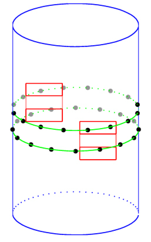
Simulation domain with two inclusions. Locations of sources and detectors are marked with black dots.

We tested a situation in which the background optical properties were known and situations in which the background optical properties were mismodelled and the true homogeneous values were 10%, 20%, 30% and 40% larger or smaller than the expected values. In all of the simulations the modulation frequency of the input signal was ω = 100MHz and the refractive index of the medium was 1.56. The absorption and reduced scattering coefficients of the background medium and the inclusions are given in Table 1 for the case 1 in which the true background optical properties were known and the case 2 in which the background optical properties were -30% off from the linearisation point x_h,0 = (μ_a,0,μ^′_s,0)^T = (0.01,1)^T.

Table 1.

The absorption coefficient μ_a(mm^-1) and the reduced scattering coefficient μ^′_s(mm^-1) of the background medium and the inclusions.

	Background		Inclusion 1		Inclusion 2
	μa	μ′s	μa	μ′s	μa	μ′s
Case 1:	0.01	1	0.04	1	0.01	4
Case 2:	0.007	0.7	0.04	1	0.01	4

The data was generated using the finite element method (FEM) with the diffusion approximation as light transport model. The data types considered were logarithm of amplitude and phase shift of the measured light. Gaussian distributed noise e with standard deviation of 0.5% of corresponding amplitude and phase was added to the simulated data.

4.1.2. Computational forward models.

For the ‘exact’ model A(x) we take a FE-approximation of the DA with a dense mesh. Let {ℕ,𝕋,𝕌} represent a set of nodes ℕ = {N_k;k = 1…n_h}, elements 𝕋 = {τ_j;j = 1…n_e}, and shape functions 𝕌 = {u_k(r);k = 1…n_h} and 𝖦 = 𝖪^-1 where 𝖪 the n_h × n_h system matrix. We used a tetrahedra mesh with n_h = 148276 nodes. For the representation of the optical parameters x_h we used 8748 cubic voxels both for absorption and scattering.

The ‘approximate’ model A_h(x_h) is taken to be

$$A_h\left(x_h\right)=G_{\infty }\left(x_{h,0}\right)+{\mathrm{�\copyright }}_{\infty }\left(x_{h,0}\right)\delta x_h$$ (33)

where G_∞(x_h,0) is the infinite domain Green’s function, Eq. (13). The Green’s function Jacobian �© = [�©^(μ_a)_∞�©^(μ′_s)_∞] is constructed by sampling the forward and adjoint fields on the same mesh node points {N_k} :

$${\mathrm{�\copyright }}_{\infty }^{\left({\mu }_a\right)}=\left(\begin{array}{ccc}⋮& ⋮& \ddots \\ \dots & G^{*}(r_k,r_{d,i})·G(r_k,r_{s,j})& \dots \\ ⋮& ⋮& \ddots \end{array}\right)$$ (34)

and

$${\mathrm{�\copyright }}_{\infty }^{\left(D\right)}=\left(\begin{array}{ccc}⋮& ⋮& \ddots \\ \dots & \nabla G^{*}(r_k,r_{d,i})·\nabla G(r_k,r_{s,j})& \dots \\ ⋮& ⋮& \ddots \end{array}\right)$$ (35)

where G^* is the adjoint Green’s function and utilising the chain rule to obtain the derivatives for the scattering. In all of the approaches, the Jacobian was calculated using the homogeneous optical properties μ_a,0 = 0.01 mm^-1 and μ^′_s,0 = 1mm^-1.

4.1.3. Approximation error statistics.

The approximation error mean and covariance were calculated similarly as in [14]. Thus, we used a proper smoothness prior model as the prior distribution π(x) and draw r = 200 samples x^(ℓ)_h from it. The correlation length for both absorption and scattering was set as 14 mm which means that this is (roughly) the prior estimate of the spatial size of the inhomogeneities in the target domain. The prior means for absorption and scattering were set as μ̄_a = 0.01 mm^-1 and μ̄^′_s = 1mm^-1, and the marginal variances for the inhomogeneity and background part were set such as 2 s.t.d. limits for the contrast of the inhomogeneities and background corresponded to 1 % of the mean values for both absorption and scattering. The approximation error was computed from the samples as

$${\epsilon }^{\ell }=A\left(x^{\left(\ell \right)}\right)-A_h\left(x_h^{\left(\ell \right)}\right)$$ (36)

where the accurate model was the FE-solution of the DA and the reduced model was the solution of the Green’s function, Eq. (33). Furthermore, the mean and the covariance of the approximation error were computed as

$$\overline{\epsilon }=\frac{1}{r}\sum _{\ell =1}^r{\epsilon }_h^{\left(\ell \right)}$$ (37)

$$\stackrel{}{{\Gamma }_{\epsilon }}=\frac{1}{r-1}\sum _{\ell =1}^r{\epsilon }^{\left(\ell \right)}{\epsilon }^{\left(\ell \right)T}-{\stackrel{}{\mathit{\epsilon \epsilon }}}^T.$$ (38)

We note that the variance of the contrast of the inhomogeneities in the prior model was chosen unrealistically small since the assumption behind the linear model needed to be fulfilled when creating the approximation error statistics. This however, as shown later in Sec. 4.2, does not limit the applicability of the approach to reconstruct larger variations in optical parameters. For more information about the Gaussian smoothness prior model, see e.g. [3,14].

Furthermore, we note that the setting up the error model is computationally intensive task and the time required is roughly the number of samples r multiplied by the time for the forward solutions of the accurate and approximative models [14]. The error model, however, needs to be estimated only once for a fixed measurement setup and it can be done off-line.

4.2. Reconstructions.

Reconstructions were calculated using three different approaches: the reference measurement correction (RM), the approximation error using first order statistics (EM-1), and the approximation error using second order statistics (EM-2).

In all of the reconstructions, the penalty functional Ψ was the proper smoothness prior model with otherwise same parameters as in creating the approximation error statistics except that the marginal variances for the inhomogeneity were set such as 2 s.t.d. limits for the contrast of the inhomogeneities corresponded to 40 % of the mean values for absorption and scattering and the marginal variances for the background part were set such as 2 s.t.d. limits for the contrast of the background corresponded to 20% of the mean values for absorption and scattering which is more realistic choice when considering absorption and scattering variations typical in DOT.

The reconstructions using the RM correction were obtained as the solution of the minimisation problem (21) where the g^obs was the simulated measurement data, g^ref was the reference data which is the FE-solution of the DA with optical properties of the linearisation point x_h,0 which were for the absorption and scattering μ_a = 0.01mm^-1 and μ^′_s = 1mm^-1 throughout the domain. Further, �©(x_h,0) was the Jacobian which was calculated as described in Sec. 4.1, Eqs. (34) and (35),using optical parameters of the linearisation point x_h,0 (μ_a = 0.01mm^-1 and μ^′_s = 1mm^-1).

The reconstructions using the EM-1 were obtained by solving the minimisation problem (24) and the reconstructions using the EM-2 were obtained by solving the minimisation problem (26). In the approaches, the approximative model A_h(x_h) was the infinite domain Green’s function, Eq. (33) and the Jacobian �©(x_h,0) was calculated similarly as in the RM. The mean and the covariance of the approximation error statistics were constructed as described in Section 4.1.

4.2.1. Reconstructions when the background properties are known.

As the first case we investigated the situation in which the background optical properties were known, thus x_h,0 = x₀, see case 1 of Table 1. Two horizontal and two vertical slices of the 3D reconstructions are shown in Figs. 2 and 3. The locations of the slices were chosen such that they cut through the inclusions.

Fig. 2.

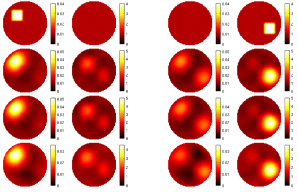
Horizontal slices at the heights z = 59mm (two columns from the left) and z = 50mm (two columns from the right) from 3D reconstructions of absorption (left) and scattering (right) distributions with known background. The images from top to bottom are: target distribution (top row), and reconstructions using RM (second row), EM-1 (third row) and EM-2 (fourth row).

Fig. 3.

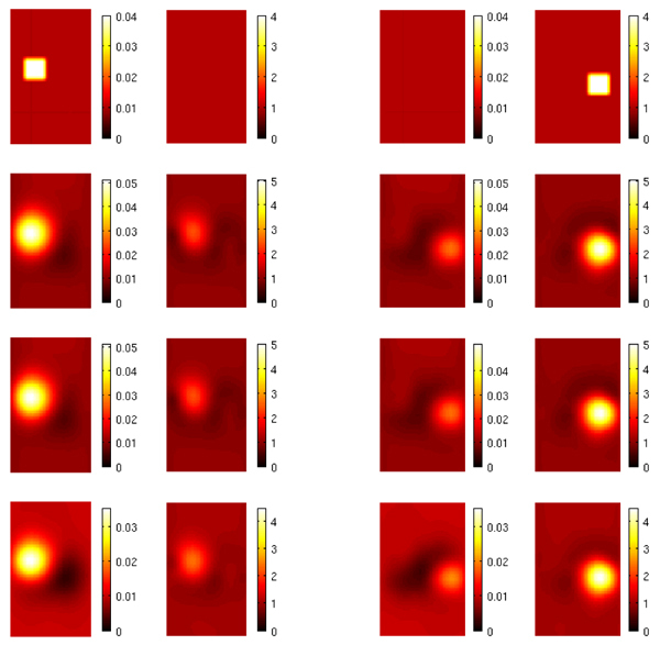
Vertical slices at the depths x = 21mm (two columns from the left) and x = 45mm (two columns from the right) from 3D reconstructions of absorption (left) and scattering (right) distributions with known background. The images from top to bottom are: target distribution (top row), and reconstructions using RM (second row), EM-1 (third row), and EM-2 (fourth row).

As it can be seen, RM, EM-1 and the EM-2 give similar results. In all of the reconstructions, the inclusions can be well distinguished and they look similar to the target distribution. Furthermore, in all of the reconstructions, the estimated absorption and scattering parameters are close to the original values. There exists some crosstalk between the absorption and scatter images. This, however, is typical for DOT reconstructions and utilising more sophisticated approximation error and prior models does not seem to reduce the amount of the cross talk in linear reconstruction as was shown to happen with the DA based reconstructions in [3].

Thus, the results show that the linear reconstruction method with a reference measurement correction can reconstruct the absorption and scattering distributions well if the background optical properties are known. On the other hand, the approximation error modelling, in which statistical properties of the modelling error are utilised instead of a reference measurement, can be used to obtain as good quality reconstructions as the reference approach.

4.2.2. Reconstructions with mismodelled background.

As the second case we investigated a situation in which the background optical properties were mismodelled. The measurement data was simulated using optical properties where the true values of the homogeneous background x₀ were 10%, 20%, 30% and 40% larger or smaller than the linearisation point (μ_a = 0.01mm^-1 and μ^′_s = 1mm^-1). The absorption and scattering values of the case 2, in which the background optical properties are 30% smaller than the linearisation point, are given in Table 1. The reference measurement g^ref, Jacobian �©(x_h,0) and the approximation error statistics were calculated using the expected optical properties x_h as described in Sec. 4.1.

Two horizontal and two vertical slices of the 3D reconstructions of the case 2 are shown in Figs. 4 and 5. The locations of the slices are the same as in the previous case of the known background optical parameters. As it can be seen, the RM and the EM-1 approaches give similar results. However, these reconstructions are unclear and the estimated optical parameters differ clearly from the values of target distribution. The EM-2 approach on the other hand, can distinguish the locations of the inclusions well. Furthermore, the optical parameters are estimated with better accuracy.

Fig. 4.

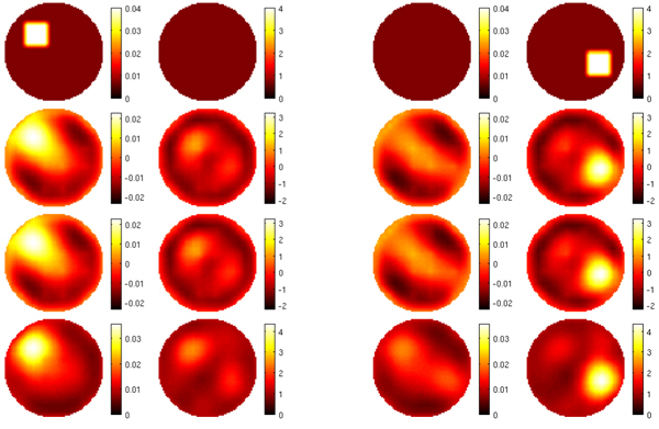
Horizontal slices at the heights z = 59mm (two columns from the left) and z = 50mm (two columns from the right) from 3D reconstructions of absorption (left) and scattering (right) distributions with mismodelled background. The images from top to bottom are: target distribution (top row), and reconstructions using RM (second row), EM-1 (third row), and EM-2 (fourth row).

Fig. 5.

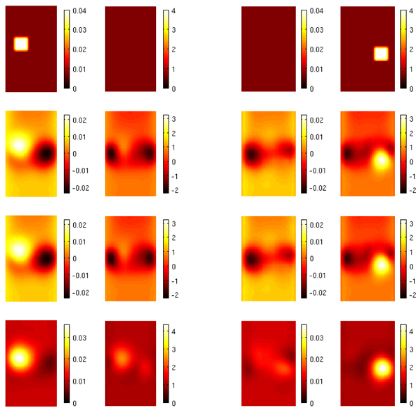
Vertical slices at the depths x = 21mm (two columns from the left) and x = 45mm (two columns from the right) from 3D reconstructions of absorption (left) and scattering (right) distributions with mismodelled background. The images from top to bottom are: target distribution (top row), and reconstructions using RM (second row), EM-1 (third row), and EM-2 (fourth row).

Thus, the results show that when the background optical properties are mismodelled, the RM and the EM-1 which both utilise only the mean of the statistical information of the error model, do not produce good quality reconstructions. On the other hand, EM-2, which takes into account correlation of the modelling errors, is capable of estimating the optical parameters with good accuracy even if the background values are 30% off from the expected ones.

4.2.3. Comparison and discussion.

To compare the capability of the different approaches to estimate the values of optical parameters, the relative errors between the target and estimated optical properties, x and x̂, respectively, were calculated as

$${\hat{e}}_x=\frac{{\parallel \left(x-\hat{x}\right)\parallel }^2}{{\parallel x\parallel }^2}·100$$ (39)

for different levels of deviation in optical parameters between the true homogeneous background and the linearisation point. The relative errors of different models against the difference in background value are shown in Fig. 6.

Fig. 6.

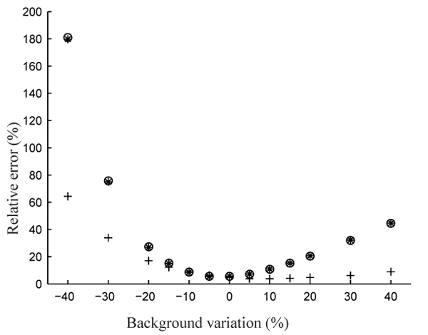
Relative errors between the target optical properties and estimated optical properties against the difference in background value calculated with the RM (∗), EM-1 (∘) and EM-2 (+).

The figure shows that when the background optical properties are known, all three approaches give similar reconstruction errors. When the error in background value compared to the linearisation point is increased, the errors of the RM and EM-1 estimates increase clearly. The errors of the EM-2 show also some increase but significantly less than the other approaches. Thus, the EM-2 method gives clearly more accurate estimates than the two other approaches and can compensate the errors caused by using mismodelled background optical properties in linear reconstruction.

5. Conclusions

In this paper we examined the correction of errors when using a first order Born approximation with an infinite space Greens function model as the basis for linear reconstruction in DOT, when real data is generated on a finite domain with possibly unknown background optical properties. We considered the relationship between conventional reference measurement correction and the approximation error modelling in DOT reconstruction. The approaches were tested with simulations in cases in which the background optical properties were known and mismodelled. The results show that when the background optical properties are known, the conventional reference correction method and the approximation error approaches using first and second order statistics give similar results, and thus all of the approaches can be used in DOT reconstruction with a linear model. However, when the background optical properties are mismodelled, the conventional reference method and the approximation error approach using first order statistics fail to give good estimates of the target optical properties. In this case, the approximation error approach using second order statistics is capable of providing feasible reconstructions of the optical properties even when the background values are 30% smaller than the expected values. Thus, the approximation error approach using second order statistics can compensate the errors caused by inaccurately known background optical properties in linear DOT reconstruction.