Semi-supervised Cluster Analysis of Imaging Data

Abstract

In this paper, we present a semi-supervised clustering-based framework for discovering coherent subpopulations in heterogeneous image sets. Our approach involves limited supervision in the form of labeled instances from two distributions that reflect a rough guess about subspace of features that are relevant for cluster analysis. By assuming that images are defined in a common space via registration to a common template, we propose a segmentation-based method for detecting locations that signify local regional differences in the two labeled sets. A PCA model of local image appearance is then estimated at each location of interest, and ranked with respect to its relevance for clustering. We develop an incremental k-means-like algorithm that discovers novel meaningful categories in a test image set. The application of our approach in this paper is in analysis of populations of healthy older adults. We validate our approach on a synthetic dataset, as well as on a dataset of brain images of older adults. We assess our method’s performance on the problem of discovering clusters of MR images of human brain, and present a cluster-based measure of pathology that reflects the deviation of a subject’s MR image from normal (i.e. cognitively stable) state. We analyze the clusters’ structure, and show that clustering results obtained using our approach correlate well with clinical data.

1. Introduction

Assigning images into groups with respect to meaningful characteristics is of significant importance in many applications. Supervised classification approaches aim at deducing a decision function from the labeled training data. This learned function, i.e. classifier, can then be used to assign novel images into known categories. For example, significant work has been done in applying pattern classification algorithms in the context of Alzheimer’s disease (AD) and mild cognitive impairment (MCI) (Duchesne et al., 2008; Fan et al., 2008; Kloppel et al., 2008; Misra et al., 2009). In the supervised analysis of medical images, patients are usually grouped under a common umbrella corresponding to high-level clinical categories (e.g. AD, MCI, autism, schizophrenia). However, in many diseases patients’ populations are highly heterogeneous. For example, the autism spectrum encompasses Autism, Asperger’s disorder, and Pervasive Developmental Disorder-Not Otherwise Specified (PDD-NOS). Additionally, a disease may evolve in a continuous manner, without going through distinct clinical stages. Figure 1 shows a diagram of two possible scenarios of patients’ distribution in many clinical studies. Clearly, the high level label information (i.e. grouping into normal and patient categories) utilized by existing supervised approaches does not present a comprehensive picture of the data structure. As a result, fully supervised approaches both fail to discover categories at finer granularity levels, and do not reflect the continuous nature of many diseases.

Figure 1.

Typical scenarios of disease evolution. Scenario 1: While patients are grouped under a common umbrella, in reality they form distinct clinical categories. Scenario 2: Disease evolves gradually, and there are no distinct clinical categories in the data. However, the level of disease progression is different for different individuals.

Problems where categorical labels are only partially available, or available only at higher granularity levels, are commonly addressed with the help of a semi-supervised learning approaches (Bensaid et al., 1996; Song et al., 2009). Semi-supervised analysis employs user-provided labels to bias the process of discovering structure in the data. Several techniques exist for incorporating prior information into semi-supervised analysis, such as seeding (inserting labeled objects into the dataset) (Basu et al., 2002), and distance metric learning (training a similarity measure using the labeled objects) (Kumar et al., 2005). Unfortunately, these semi-supervised techniques often assume that both labeled and non-labeled data come from the same distributions. Moreover, it is unclear how the labeled information can be incorporated into an unsupervised pattern discovery process if the data under consideration does not contain categories provided by the partial labels. As an example, consider the task of clustering normal older participants into meaningful categories (e.g. the ones that will develop a cognitive impairment in the future and the ones that will not). As none of the healthy individuals is diagnosed with MCI, it is not immediately evident how the labels of healthy and MCI subjects can guide the process of analyzing the structure of the healthy cohort.

Clustering is a popular form of unsupervised and semi-supervised learning, and seeks to determine how the data is organized. A multitude of clustering algorithms were proposed to date that can be divided into those that assume that the number of clusters is known beforehand, and those that automatically determine the number of clusters in a dataset (i.e. unsupervised clustering algorithms). As there is often not enough prior knowledge about the specific categories that the clustering algorithm should reveal, the unsupervised clustering algorithms are particularly appealing.

The data in many real-life applications is high-dimensional and, due to the curse of dimensionality, cannot be readily analyzed. The dimensionality reduction can be achieved by extracting a small set of features from descriptive anatomical regions. These descriptive image neighborhoods can be detected by considering local region saliency (Lindeberg, 1993), intergroup correlation (Fan et al., 2007), etc. Approaches that find neighborhoods signifying intergroup differences are particularly appealing as they allow incorporation of prior information in the form of labeled image sets.

In order to examine spatial patterns across individuals there is a need to establish a unified coordinate systems across all images. Registering images to a common template allows association of measurements across images, and often serves a purpose of signifying local deviations from a template (Davatzikos et al., 2001; Zitova, 2003). While image registration is often used in medical image analysis (Zitova, 2003), it is also common in other imaging problems (e.g. face recognition (Jia et al., 2006), astrophotography (Mink, 1999), etc.).

In this paper, we present a semi-supervised approach to discovering coherent subpopulations in image sets. We specifically target the problems where subjects populations are heterogeneous, or when a disease evolves in a continuous manner. The former problem is addressed naturally by using a semi-supervised clustering approach. In the case of normal elderly populations when there are possibly no distinct subpopulations in the dataset, we show that denser subpopulations of normal older adults may correspond to individuals with better cognitive performance. By iteratively removing dense subpopulations from the data, we isolate patient subpopulations of increasing levels of pathology. Our approach differs from the existing classification methods applied to studies of elderly populations in that rather than attempting to classify individuals into known diagnostic categories, we attempt to understand the heterogeneous structure of the elderly populations, and, possibly, discover novel categories in it.

We hypothesize that the local regions reflecting differences between images in two labeled sets will also be discriminative for clustering images that belong to novel categories. By the term “image region” we understand a group of neighboring locations (i.e. voxels) in the image. We propose a method for estimating local appearance models around the locations that signify regional differences in the two labeled sets. Additionally, we incorporate a feature ranking strategy that weights local neighborhoods with respect to their relevance for clustering. We develop an incremental k-means-like clustering algorithm that employs a merging procedure to automatically determine the number of clusters in the dataset. Finally, we validate our approach on both synthetic and real datasets. We assess our method’s performance on the problem of discovering clusters of MR images of human brain, and present a cluster-based measure of pathology that reflects the level of abnormality of a subject’s MR image. We analyze the clusters’ structure, and show that clustering results obtained using our approach correlate well with clinical data. The flowchart of our approach is presented in Figure 2 and depicts the main steps in our semi-supervised clustering algorithm.

Figure 2.

Flowchart of our approach. The supervised part of the input consists of two groups used to detect features that may be useful for clustering. In the feature detection step, regions of high intergroup differences are first obtained by segmenting KL-divergence map obtained from the two groups. For each region, a location (i.e. voxel) that corresponds to the highest intergroup difference value is selected and the appearance model is learned in its neighborhood. Only those locations and corresponding appearance models that are “relevant” for clustering are retained. These locations and appearance models are then used to obtain feature-vector representation of the new data. If dimensionality of the extracted feature vectors is large, it is reduced using a manifold learning technique. Finally, the data is being clustered using a version of ISODATA algorithm.

The remainder of this paper is organized as follows. In Section 2, we detail the main components of our interest region detection process. In Section 3, we describe the clustering algorithm used in our framework. We present our experimental results in Section 4. Finally, conclusion and discussions are provided in Section 5.

2. Estimating Appearance Models at the Discriminative Locations

In real-life scenarios some types of data labels may be more reliable than others. Additionally, labels for some image categories may be missing during training. At the same time, labeled subject populations are often grouped into two categories, with one corresponding to healthy individuals (e.g. normal controls), and another being a subgroup of patients with disease (e.g. AD, autism). Our main hypothesis is that image locations signifying differences between the labeled groups of healthy and patients, are also suitable for clustering unlabeled images into novel categories. These categories may correspond to finer granularity levels in healthy or non-healthy groups, or to the various stages of disease, as individuals progress from healthy to diseased. For example, when analyzing image clusters of individuals with mild cognitive impairment (MCI), one may expect the regions that distinguish between the normal individuals (NC) and individuals with Alzheimer’s’ disease (AD), to be also suitable for clustering MCI subjects into potential progressors and nonprogressors.

In this section, we present an approach that utilizes information from two labeled subsets of images to estimate local appearance models at the locations corresponding to large regional intergroup differences. This supervised stage of our approach consists of the following steps:

1. Detecting point-wise regions of intergroup differences. In this step, initial regions are obtained that reflect the intergroup point-wise differences between two sets of labeled images.

2. Local PCA models estimation. Here, for each initial region, a PCA model of local appearance is estimated in the neighborhood of locations corresponding to the highest value of intergroup differences.

3. Ranking interest regions. In this step, regions of interest are ranked with respect to their relevance for clustering.

The steps of the supervised stage are detailed next.

2.1. Detecting point-wise regions of intergroup differences

As it was mentioned earlier, the high data dimensionality must be reduced to a relatively small set of descriptive features. Unlike point-wise measurements, regional measurements are always more robust to appearance variations due to noise and global transformations. Consequently, our goal is to detect image subregions that have the most potential to be useful for clustering unknown categories.

In order to identify regions of interest (ROI), we begin by assuming the availability of two sets of labeled images ${\mathcal{I}}_1=\{I_1^1,\dots ,I_{S_1}^1\}$ and ${\mathcal{I}}_2=\{I_1^2,\dots ,I_{S_2}^1\}$. These training sets reflect our guess about the differences that the clustering algorithm should emphasize on. For example, sets ${\mathcal{I}}_1$ and ${\mathcal{I}}_2$ may correspond to images from the group of normal controls and the group of patients. In the task of clustering normal elderly populations considered in this paper the two sets correspond to the normal adults with good cognitive performance and MCI patients.

We use Kullback-Leibler (KL) divergence to evaluate the group-wise differences at a given image location. KL divergence is a common measure of the difference between two probability distributions, and measures the expected number of extra bits required to code samples from one distribution when using a code based on another distribution. In the case of normal distributions, unlike t-test which emphasizes the difference in means, KL-divergence places importance in both their means and their variances.

The KL divergence at location u has the following form:

$$K{L}_{q,p}\left(u\right)={\int }_{-\infty }^{\infty }p\left(x\right)\log \frac{p\left(x\right)}{q\left(x\right)}dx$$ (1)

where, x is an image descriptor at location u, and p(x) and q(x) are the probability densities of measurements at location u in the first and second labeled sets, respectively. While the method presented in this paper is general and its presentation does not depend on specific type of input, in our experiments we used a tissue density preserving approach to preprocess the raw MRI data. As a result, image descriptor x in our specific experiments indicates the value of gray matter tissue density.

Estimating KL divergence for every location in the image results in a group differences map where higher values indicate higher point-wise difference between two labeled sets. Adjacent locations with high KL-values can be grouped into regions using a segmentation algorithm. In our implementation, we followed (Fan et al., 2007), and used the watershed algorithm to partition an image into regions according to the similarity of point-wise KL divergence values.

As the result of segmenting the KL divergence map, we obtain a set of L regions {R₁, …, R_L} of high intergroup point-wise differences. A simple way to use the segmentation-derived regional elements for a specific image would be to average all intensity values in each region, yielding a regional measure corresponding to a specific region in the image. Such regional measures from all regions could constitute a feature vector to represent appearance information of the image, which is robust to noise, global transformations, and inter-image appearance variation (Fan et al., 2007). However, using all points in the region to compute a regional measure might reduce the discriminative power of this region, since the regions R_l may include points of varying intensity, while at the same time having similar KL divergence values. As a result, simplistic regional measures may not be suitable for clustering. On the other hand, the segmentation-based partitioning can provide a good initialization for selecting an appropriate subregion from each segmented region.

2.2. Local PCA models estimation

As discussed above, large region sizes may lead to overly complex distributions of intensity values inside corresponding subregions. At the same time, if the regions are too small, the volumetric measures become sensitive to noise. In order to address these issues, for a given region R_l, we define location ${\tilde{u}}_l$ corresponding to the maximum value of KL-divergence in R_l

$${\tilde{u}}_t=\underset{u\in R_t}{\text{arg max}}K{L}_{q,p}\left(u\right)$$ (2)

By choosing a single location for every region we keep the overall number of locations ${\tilde{u}}_l$ in the image small. For example, the tissue density maps considered in our experiments are of the size 96 × 113 × 94. As the result of segmenting the KL divergence map, we obtain about 10³ regions, and hence, as many locations ${\tilde{u}}_l$ (i.e. one location of interest per region). This number is significantly smaller than the original dimensionality of the data.

Intuitively, the immediate subregion around the location corresponding to the highest value of KL divergence has the most potential to reflect the intergroup differences in the test set. For j-th training image and at location ${\tilde{u}}_l$, we extract a square (or cuboid in case of 3-D images) subregion ${\mathcal{R}}_{l,j}$ of standard size. For example, in our real-life experiments the size of the subregions was selected to be 5 × 5 × 5 voxels. Although the image values in ${\mathcal{R}}_{l,j}$ describe the neighborhood of the point with the largest group difference in R_l,j, the distribution of intensity values in ${\mathcal{R}}_{l,j}$ may still be multivariate disallowing usage of simplistic regional statistics. This is particularly evident for the cases where the disease is accompanied by increased intensity values in one regions and decreased intensity values in others. In the worst-case scenario, simple averaging over a combination of such regions may cancel our the effect of pathology. Consider, for example, intensity values corresponding to tissue density values. Existing studies suggest that AD may be accompanied by both disease-like patterns of brain atrophy, primarily in the temporal lobe, and increase in estimated gray matter in periventricular regions highlights regions of greater white matter abnormalities (Davatzikos et al., 2009). As the result, for AD-like subjects one can observe regions of increased tissue density as well as regions of decreased density. The problem may become even more pressing for studies of autism, where there may be multiple neighboring brain regions of increased and decreased brain matter (Akshoomoff et al., 2002; McAlonan et al., 2005).

Alternatively, principal component analysis (PCA) presents a simple, yet effective, procedure for revealing the internal structure of the data in a way which best explains the variance in the data. In our approach, for a given location ${\tilde{u}}_l$ we extract intensity values from all subregions ${\mathcal{R}}_{l,j}$. We then estimate a PCA model ${\mathcal{M}}_l$ of the extracted data, where the first principal components in ${\mathcal{M}}_l$ account for most of the variability in the subregion data. In this way, ${\mathcal{M}}_l$ represents the local appearance model in the neighborhood of ${\tilde{u}}_l$. While the size of the subregions ${\mathcal{R}}_{l,j}$ and the number of retained principal components in the appearance model have to be selected in advance, our experiments suggest that the results presented in this paper are relatively stable with respect to the choice of these two parameters.

As the result of this step, we obtain a set of L locations ${\tilde{u}}_l$ with a set of corresponding PCA models ${\mathcal{M}}_l$. The pairs ($({\tilde{u}}_l,{\mathcal{M}}_l)$) can now be used to obtain a feature-vector representation V of a novel image by extracting subregions at locations ${\tilde{u}}_l$, and by projecting the extracted data onto the first n principal components of the corresponding PCA models. However, different pairs of locations ${\tilde{u}}_l$ and corresponding PCA models will most likely result into PCA projections with different descriptive power. In order to assess the relevance of individual locations for clustering, we use the relevance estimation procedure described next.

2.3. Ranking interest regions

Findings in the area of high-dimensional clustering suggest that not all subspaces of the original vector space are equally relevant for clustering (Agrawal et al., 2005; Baumgartner et al., 2004; Bohm et al., 2004). In order to estimate the clustering ability of the pairs ($({\tilde{u}}_l,{\mathcal{M}}_l)$), we adopt the quality criterion originally proposed in (Baumgartner et al., 2004). However, unlike (Baumgartner et al., 2004) we do not estimate the clustering quality of individual dimensions in feature vectors V, but measure the clustering relevance of locations ${\tilde{u}}_l$. Additionally, in our experiments, we found that clustering quality at the specific locations is more relevant if estimated from the labeled data, rather than from the test data. This can be explained by the fact that labeled data usually corresponds to a pair of well-defined clusters, and thus, the ranking procedure can easier determine locations suitable for clustering labeled images. At the same time, the dataset considered in this paper does not have clearly defined clusters, and, hence, the ranking procedure may be misguided if applied directly to the clustered data.

We proceed by projecting the data extracted in the neighborhood of ${\tilde{u}}_l$ from all training images in ${\mathcal{I}}_1\cup {\mathcal{I}}_2$ onto the first n PCA components of ${\mathcal{M}}_l$. This results in a set of n-dimensional vectors $\mathcal{W}=(w_1,\dots ,w_{s_1}+s_2)$. For a given $k\in \mathbb{N}$, let NN(w_s) be a set of k-nearest neighbors of the projection vector w_s. Additionally, let d_nn(w_s) be the distance between w_s and its k nearest neighbors, and defined as follows:

$$d_{nn}\left(w_s\right)=\text{max}\{d(w_s,w_i)\mid w_i\in NN\left(w_s\right)\},$$ (3)

where d(w_s, w_i) is the Euclidean distance between w_s and w_i. For comparability purposes, the values d_nn(w_s) are scaled to be in the range d_nn(w_s) ∈ [0, 1].

The k-nearest neighbors distance (k-nn distance) of w_s indicates how densely the elements from $\mathcal{W}$ are populated around w_s. The smaller the value of d_nn(w_s), the denser is the distribution of elements around w_s. An important observation is that for uniformly distributed elements in $\mathcal{W}$, the k-nn-distances of elements will be almost equal. On the other hand, if $\mathcal{W}$ contains clusters with different densities and noise objects, the k-nn-distances should be different. As the result, the presence of significantly different k-nn-distances suggests higher relevance of PCA projections around location ${\tilde{u}}_l$. A theoretical weakness of the measure in Equation 3 can be observed in the case of several ideally separated clusters without noise. If the separation between the noiseless clusters is large, the values d_nn(w_s) will be nearly constant, erroneously suggesting irrelevance of the location for clustering. However, in the real data we have found this criterion to work well. Our experiments showed that even without considering these extreme cases, the use of the described quality indeed improves clustering performance.

A good measure of differences in d_nn(w_s) is based on the sum of absolute differences of each d_nn(w_s) to the mean k-nn-distance μ_NN. This measure is given by

$$\alpha =\frac{1}{2}\underset{w\in \mathcal{W}}{\Sigma }\mid {\mu }_{NN}-d_{nn}\left(w\right)\mid .$$ (4)

The measure in Equation 4 can be further scaled by μ_NN times the number of elements having smaller k-nn-distance than μ_NN, i.e. the elements from the following set:

$$\mathcal{B}=\{w\in \mathcal{W}\mid d_{nn}\left(w\right)<{\mu }_{NN}\}.$$ (5)

Finally, the clustering quality at given location is calculated as:

$$Q=\{\begin{array}{cc}0\hfill & ,if\mid \mathcal{B}\mid =0\hfill \\ \frac{\alpha }{\mid \mathcal{B}\mid .{\mu }_{NN}}\hfill & ,\text{otherwise},\hfill \end{array}\phantom{\}}$$ (6)

where $\mid \mathcal{B}\mid$ indicates the number of elements in $\mathcal{B}$, and Q is in the range between 0 and 1.

As the result of the clustering relevance estimation procedure, we obtain a quality value Q_l for every location ${\tilde{u}}_l$. A lower quality value indicates less interesting clustering structure at location ${\tilde{u}}_l$, while large Q_l suggests that the corresponding location is more relevant for clustering. We can now retain only M highest-ranked locations where M < L, and perform clustering of the feature vectors extracted from the test images at the retained locations. Next, we describe the details of our clustering algorithm.

3. Incremental Clustering

The ROI estimation stage presented in Section 2 results in a set of M locations ${\tilde{u}}_m$ with a set of corresponding PCA models ${\mathcal{M}}_m$. The pairs ($({\tilde{u}}_m,{\mathcal{M}}_m)$) can now be used to obtain a feature-vector representation of a novel image by extracting standard subregions at locations ${\tilde{u}}_m$, and by projecting the extracted data onto the first n principal components of the corresponding PCA models ${\mathcal{M}}_m$. After concatenating all PCA projections for all M locations ${\tilde{u}}_m$ in the image, we obtain a feature-vector representation V of the image. In this way we can extract a set of feature vectors $\mathcal{V}=\{V_1,\dots ,V_S\}$ from a set of S test images.

Our task is to use a clustering method to discover categories in a set of images with the goal of better understanding the structure of the data at hand. More specifically, we want to discover clusters in $\mathcal{V}$ that correspond to instances exhibiting similar imaging profiles. Unfortunately, there is often not enough prior knowledge about the specific categories that the clustering algorithm should reveal. This is particularly evident in the problems where the properties with respect to which the data can be grouped are not known beforehand. As the result, the number of clusters in the set of images is not provided, and the task of the clustering algorithm is to reveal the internal structure of the data under consideration.

In our approach, we follow the unsupervised clustering strategy of Iterative Self-Organizing Data Analysis Techniques (ISODATA) to perform cluster-based analysis of MRI data. While we tried a number of clustering approaches, ISODATA provided the most consistent performance on the task of grouping MCI-like patients into a single category. Quantitative evaluation of alternative algorithms is provided in the experiments section of this paper.

Various ISODATA approaches extend k-means clustering algorithm by adding splitting and merging of clusters (Jensen, 1995). Clusters are merged if either the number of elements in a cluster is less than a certain threshold, or if the centers of two clusters are closer than a certain threshold. Clusters are split into two different clusters if the cluster standard deviation exceeds a predefined value and the number of members is twice the threshold for the minimum number of members. The ISODATA algorithm is similar to the k-means algorithm with the distinct difference that the ISODATA algorithm automatically determines the number of clusters, while the k-means assumes that the number of clusters is known a priori.

While traditional ISODATA algorithm has the advantage of being unsupervised, it requires a number of parameters to be empirically chosen. The standard deviation threshold used for splitting clusters is the least intuitive and most difficult to select. In order to reduce the number of parameters in the traditional ISODATA algorithm, we do not incorporate the cluster splitting procedure into the clustering algorithm. Instead, starting with a large number of small clusters, our algorithm performs iterative merging until the stopping criteria are met. Algorithm 1 in the appendix provides details of the ISODATA procedure used in our approach.

Although, the algorithm takes as its input the desired number of clusters K, there is no guarantee that exactly K clusters will be produced. Instead, K serves as a rough preference for the granularity of the resulting grouping. When K is large, the algorithm will prefer a larger number of small clusters, and will tend to produce a small number of larger clusters if K is small. Additionally, discarding of too small clusters in Line 3 of Algorithm 1 may lead to the cases when not all elements are assigned to clusters. In order to achieve cluster assignment for all elements, we perform a post-clustering step where each unassigned element is being associated with a cluster corresponding to the centroid closest to that element.

4. Experimental Results

4.1. Data Description

In order to assess the validity of our proposed approach, we performed a set of simulated and real-data experiments. The datasets used in our experiments are described next.

4.1.1. Simulated data

Simulations enable us to generate images that come from precisely known distributions. This allows us to quantitatively assess the performance of our clustering algorithm. To this end, we selected a template ribbon shape that represents a common morphology in the cortex of human brain. In order to simulate atrophy of the brain cortex, we manually selected regions of thinning in the template image. Thinning of the ribbon simulates atrophy of the brain cortex, and was achieved by performing morphological operations. In our experiments, the amount of thinning was parameterized by Gaussian mean and variance. Example template image and the selected thinning regions are shown in Figure 3(a,b).

Figure 3.

Simulated data generation process. (a) Template image; (b) Two thinning regions; and (c) Variance in the simulated dataset due to global transformations.

We applied random scaling and rotation transformations to simulate global errors in the tissue registration process. Finally, we applied Gaussian smoothing to the simulated images. Figure 3(c) shows the dataset variance induced by global transformations. It can be seen from Figure 3(c), that due to the global transformations in the images, regions with high variance occur in the nonthinned areas (i.e. right-top end of the ribbon). Similar noise variance often occurs in real-data, where registration errors may confuse the analysis. Some example simulated images with varying levels of atrophy are shown in Figure 4.

Figure 4.

Example simulated images corresponding to varying levels of atrophy.

We simulated three different levels of atrophy by selecting distinct means governing the the distributions of thinning parameters (i.e. μ₁ for low atrophy, μ₂ for medium atrophy, and μ₃ for high atrophy). Different levels of simulated atrophy reflect the fact that some diseases may evolve through a set of distinct stages. Additionally, if thinning parameters μ₁, μ₂, and μ₃ are significantly different, then the corresponding atrophy stages are distinct. In contrast, similar values of μ₁, μ₂, and μ₃ indicate that atrophy evolves in a continuous manner. We generated simulated images using different sets of thinning parameters, and assessed the performance of our approach when the distinctiveness of atrophy stages decreases. For every set of thinning parameters, we generated 20 images with lower atrophy level, and 20 images with higher atrophy level. These images served the purpose of guiding the feature detection process described in Section 2. Additionally, we generated 150 images representing the three levels of atrophy (i.e. 50 images for each atrophy level). These 150 images were subsequently clustered following the procedure described in Section 3.

4.1.2. Real MR brain images from the Baltimore Longitudinal Study of Aging

The Baltimore Longitudinal Study of Aging (BLSA) is a prospective longitudinal study of aging. Its neuroimaging component, currently in its 16th year, has followed 158 individuals (age 55-85 years at enrollment) with annual or semi-annual imaging and clinical evaluations. The neuroimaging substudy of the BLSA is described in detail in (Resnick et al., 2003). At the time of development of this paper the dataset contained 975 scans that had associated cognitive evaluations. Eighteen participants were diagnosed with MCI over the course of the study. There were 93 scans with associated cognitive evaluations of MCI participants.

Cognitive evaluations

To determine the relationship between our clustering results and cognitive performance, we examined the clustering results obtained with our approach in relation to performance on tests of mental status and memory. From the battery of neuropsychological tests administered to participants in conjunction with each imaging evaluation, we selected four measures for analysis. The four measures used in the current analyses were the total score from the Mini-Mental State Exam (MMSE) (Folstein et al., 1975) to assess mental status, the immediate free recall score (sum of five immediate recall trials) on California Verbal Learning Test (CVLT) (Delis et al., 1987), and the long-delay free recall score on CVLT, to assess verbal learning and immediate and delayed recall, and the total number of errors from the Benton Visual Retention Test (BVRT) (Benton, 1974) to assess short-term visual memory. We focused on these measures because changes in new learning and recall are among the earliest cognitive changes detected during the prodromal phase of AD (Grober et al., 2008).

4.1.3. Preprocessing MRI data

All MR images were preprocessed following mass-preserving shape transformation frame-work (Davatzikos et al., 2001). Each skull-stripped MR brain image was first segmented into three tissues, namely gray matter (GM), white matter (WM), and cerebrospinal fluid (CSF), by a brain tissue segmentation method proposed in (Pham and Prince, 1999). Afterwards, each tissue-segmented brain image was spatially normalized into a template space, by using a high-dimensional image warping method (Shen and Davatzikos, 2002). The total tissue mass is preserved in each region during the image warping, which is achieved by increasing the respective density when a region is compressed, and vice versa. Finally, tissue density maps were generated in the template space, reflecting local volumetric measurements corresponding to GM. An example of tissue density map for GM is shown in Figure 5. These tissue density maps give a quantitative representation of the spatial distribution of tissue in a brain, with brightness being proportional to the amount of local tissue volume before warping.

Figure 5.

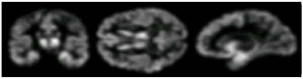
Example of smoothed tissue density map of GM.

4.2. Analysis

4.2.1. Clustering simulated data

As has already been mentioned, the simulated thinning of regions in 2-D shapes represents presence of different types of atrophy. The aim of our simulated experiments is to determine whether our clustering approach can separate groups with different types of simulated atrophy. In our experiments, we performed the training stage of our approach using 40 training images (i.e. 20 images with low atrophy level, and 20 images with high atrophy level). Following the training procedure in Section 2, we detected locations of interest, and built local PCA appearance models using the data extracted from the detected locations’ neighborhoods of dimensions 5 × 5. Only the first two principal components were used for projecting local regional data. A clustering relevance value was associated with every point, with higher values corresponding to locations that are likely to be useful for clustering. At the test stage, we extracted image features using locations and local PCA models obtained during training.

We assessed the ability of our algorithm to cluster test images into three groups according to the level of atrophy. A complete simulated experiment consists of data generation, feature detection, and clustering. As discussed earlier, significantly different levels of atrophy in the dataset indicate presence of distinct stages of disease. We repeatedly performed the complete experiment for different triplets of means governing thinning parameters distributions. That is, for a specific triplet of parameters means we generated training images and test images, and feature detection and clustering was performed using the generated images. The process of image generation, feature detection, and clustering was repeated 50 times. By adjusting the parameter corresponding to the desired number of clusters in the clustering algorithm, we obtained three clusters at each complete simulated experiment. A cluster can be assigned a label based on the atrophy level of the majority of the elements in the cluster. Ideally, one would hope to find three clusters, with a specific cluster containing images with the same atrophy level.

Clustering results as observed for varying dissimilarity between atrophy levels in the dataset are shown in Figure 6.

Figure 6.

Evolution of clustering accuracy with atrophy distinctiveness. The horizontal axis represents difference between thinning parameter distributions. Thinning parameter distributions for some experiments are also shown. Intuitively, highly overlapping distributions indicate absence of distinct clusters in the dataset.

As expected, if atrophy levels in the three groups are similar (i.e. parameter distributions are overlapping), the algorithm fails to discover the three atrophy classes. On the other hand, for significantly different atrophy levels, the algorithm can achieve near perfect performance even in presence of confusing global transformations. Nevertheless, data noise seems to affect the clustering performance when the distinctiveness of atrophy groups approaches the middle of the considered spectrum of atrophy triplets.

4.2.2. Clustering BLSA brain images

In the next set of experiments, we tested the performance of our approach on the images from the BLSA dataset. The main goal of our experiments was to examine the structure of the data in the BLSA study. Cluster analysis of the BLSA data is a challenging task as a subject’s cognition usually degrades in a continuous manner. Additionally, we explored ways of using discovered subpopulations to quantify the severity of pathology in individual brains.

In the interest region detection stage of our algorithm one needs to identify two training subsets that could potentially yield features that are relevant for clustering. Ideally, the two training subsets would belong to different ends of disease spectrum, with one subset corresponding to participants with better cognitive performance and the other subset corresponding to participants that are cognitively declined. We selected 50 MRI scans of 8 subjects diagnosed with MCI to represent the cognitively declined subset. We used cognitive scores to identify a subset of normal adults that may show relatively better cognitive performance. Specifically, we selected 50 images of 7 participants in such a way, that the average MMSE score and the average CVLT List A score of the selected participants at the first visit was above average of the first-visit evaluations. It is obvious that many alternative strategies for selecting the two training sets are possible, and care has to be taken to ensure the two selected sets allow to detect features that a relevant for clustering.

The remaining 875 scans were retained for clustering and included 43 MCI images that did not take part in feature detection. The presence of some scans of MCI subjects allowed us to judge the clustering performance of our algorithm as described later in this paper.

During the interest region detection stage of our approach, we learned local PCA models in the 5 × 5 × 5-voxels neighborhoods of locations of interest. We used only the first two PCA components of local models. After ranking detected locations with respect to their relevance for clustering, we retained only half of top ranked locations and corresponding local PCA models. We then extracted feature vectors from the images retained for clustering, resulting in 875 feature vectors of dimensionality being approximately 10³. Example of 10³ top-ranked detected locations and their immediate neighborhoods are shown in Figure 7. In the figure, the neighbourhoods are colored with respect to their relevance for clustering. Notice that, while there is a relatively large number of detected locations in the occipital lobe, which is not commonly associated with age-related cognitive decline, they have low clustering relevance values.

Figure 7.

Example of 10³ top-ranked detected locations signifying differences between cognitively stable and cognitively declined subjects in the BLSA study. The neigbourhoods of the detected locations are colorcoded with respect to their relevance for clustering. For display purposes, the values of clustering relevance for the top 10³ locations where normalized to be within the unit interval. Higher values of the color map indicate higher relevance.

The high dimensionality of the feature vectors obtained at this point may prevent the clustering algorithm from producing reliable results. At the same time brain images can sometimes be assumed to be lying on a low-dimensional manifold embedded in a high-dimensional space (Batmanghelich and Verma, 2008; Khurd et al., 2006). The problem of discovering true intrinsic dimensionality of the manifold can be approached with manifold learning techniques like ISOMAP (Tenenbaum et al., 2000) or Locally Linear Embedding (LLE) (Roweis and Saul, 2000). The ISOMAP algorithm forms a graph by connecting each point to its nearest neighbors, approximates pairwise geodesic distances on this graph, and applies metric mutidimensional scaling (MDS) to recover a low dimensional isometric embedding. In our experiments ISOMAP failed during the MDS step. Therefore, we resorted to LLE which works by computing nearest neighbors of every point, solving for the weights necessary to reconstruct each point using a linear combination of its neighbors, and finding a low dimensional embedding that minimizes reconstruction loss. As a result of applying LLE, we reduced vector dimensionality to 20.

We performed clustering of the data using our incremental approach. Our algorithm discovered two clusters of significantly different sizes (i.e. 855 and 20 elements respectively). Notably, all 43 MCI scans belonged to the larger cluster. Following this observation, we hypothesized that subjects’ brains in a larger cluster may have overall higher levels of pathology than the subjects in the smaller cluster. This in turn would mean that the image population of subjects with relatively better cognitive performance is more densely distributed than the population of less normal brain images.

4.2.3. Hierarchical structure of the data

In order to further analyze the structure of the data, we performed several iterations of the clustering algorithm, where at each iteration we obtained subclusters of the larger cluster found at the previous iteration. At each iteration, the algorithm yielded two subclusters, one large subcluster and one relatively small. A part of the hierarchy of obtained subclusters and corresponding subcluster sizes are shown in Figure 8.

Figure 8.

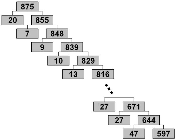
Hierarchical structure of the BLSA data. Numbers in the boxes indicate the number of elements in corresponding subclusters.

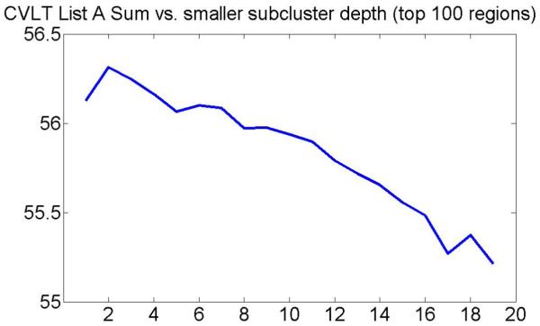
Next, at each level of the hierarchical clustering structure in Figure 8, we calculated mean cognitive scores and mean age. The plots showing evolution of different mean cognitive scores in smaller subclusters with the subcluster depth are presented in Figures 9(a-d). This is an important result, suggesting that more normal brains usually form tighter clusters, and that cognitive scores usually worsen with the cluster depth.

Figure 9.

Evolution of mean cognitive scores in smaller subclusters with the subcluster depth.

Additionally, the hierarchical structure of clusters in the BLSA dataset (Figure 8) indicates that there are no clearly defined clusters. This supports the hypothesis that brain morphology degrades in a continuous manner.

4.2.4. Effect of the choice of parameters

As described in Section 2.2, during the feature detection stage of our algorithm one needs to select the size of standard subregion and the number of principal components that encode local appearance in the subregion. We performed a set of experiments to assess the effect of choosing these parameters. In particular, we varied the parameters and evaluated the evolution trends of mean cognitive scores in smaller subclusters with the subcluster depth.

The plots in Figures 10 and 11 show evolution of mean CVLT List A Sum in smaller subclusters with the subcluster depth for different parameters of the appearance model estimation step. The results are consistent with the mean score evolution initially shown in Figure 9(a), and once again suggest that clusters of normal elderly adults at the higher levels of hierarchy may correspond to subpopulations with better cognitive performance. As the result, we retain only the first two principal components for the remaining experiments described in this paper. This choice results in a smaller size of feature vectors and reduces computation time of our approach.

Figure 10.

Evolution of mean CVLT List A Sum in smaller subclusters with the subcluster depth for different choices of standard subregion size.

Figure 11.

Evolution of mean CVLT List A Sum in smaller subclusters with the subcluster depth for different choices of the number of retained principal components in the appearance model.

4.2.5. Cluster-based level of pathology

While the obtained clusters give us understanding of the image set structure, it is also desirable to be able to quantify the amount of atrophy in an individual brain. Given a cluster of images with higher pathology C_P, and a cluster of more normal images C_N, we propose to define the level of pathology for an image represented with a feature vector V as follows:

$$\mathcal{D}\left(V\right)=d(V,{\mathbf{m}}_N)-d(V,{\mathbf{m}}_P),$$ (7)

where d(V, m_N) and d(V, m_P) are the distances from V to the centroids of more normal and more pathological clusters, respectively. As the result, we expect individuals with better cognitive performance to have lower level of pathology, and vice versa.

In our experiments, we used the centroids of two clusters obtained at the highest hierarchical level to calculate the level of pathology in Equation 7. Having calculated the level of pathology for every image in the dataset, we can asses the validity of the proposed measure by analyzing the correlation between the measure and cognitive scores.

4.2.6. Relationship between level of pathology and cluster hierarchy

We calculated mean level of pathology for the smaller subclusters in the cluster hierarchy. Figure 12 shows a plot of evolution of the level of pathology with the cluster depths.

Figure 12.

Evolution of mean level of pathology in smaller subclusters with the subcluster depth.

The plot suggests that, at each iteration, our algorithm “peels off” a subset of images with the lowest level of pathology. This small and dense subset of images corresponds to the most normal subpopulation at the specific iteration. This implies that the BLSA data looks more like “Scenario 2” in Figure 1.

4.2.7. Relationship between cognitive performance and level of pathology

In order to analyze the relationship between the level of pathology and clinical performance, we divided individuals into two groups with respect to their mean level of pathology. One group was formed out of individuals having mean level of pathology values in the upper quartile (i.e. upper 25%). The subjects with the lower 75% of the mean level of pathology were placed into the second group. Analysis of groups that correspond to the extreme quartiles of the pathology values is similar to the analysis of classification-based biomarkers of AD (Davatzikos et al., 2009), where only the extreme quartiles of the real-valued biomarkers can be considered when assessing relationships with cognitive performance.

We performed cross-sectional analyses of the four cognitive measures (CVLT Sum of Immediate Free Recall, CVLT Delayed Free Recall, BVRT errors, and MMSE) in relation to the mean level of pathology. Cognitive performance between groups was compared by one-sided t-test.

As shown in Table 1, dividing participants with respect to the mean level of pathology yields two groups, where subjects in one group usually have significantly better cognitive scores than subjects in the other group. Only for BVRT Error at the first visit there was no significant group difference observed. Overall, the results in Table 1 suggest that clusters obtained using our approach allowed us to define a measure of level of pathology in human brain. Additionally, we did not observe significant age difference between the lower and the upper quartile groups (p=0.322). This suggests that our method captured pathology that is not solely induced by age.

Table 1.

Relationship between cognitive performance and mean level of pathology

	CVLT List A Sum	CVLT Long Delay Free	BVRT Errors	MMSE
Mean Scores	0.001	<0.001	0.007	0.048
First Visit Scores	0.001	0.001	0.011	0.137
Last Visit Scores	<0.001	0.001	0.042	0.038

p-values of one-sided t-test obtained for the group with mean level of pathology in upper 25% vs. the group with mean level of pathology in lower 75%.

Additionally, we performed voxel-wise t-tests to compare the image groups corresponding to the upper and lower quartiles of the level of pathology (upper 25% vs. lower 25%). The corresponding group differences are shown in Figure 13. The figure shows p-vales of one-sided t-test obtained for two groups, and suggests that there is significant loss of brain matter in individuals with associated higher level of pathology.

Figure 13.

Voxel-wise differences in groups corresponding to lower and upper quartiles of level of pathology. The images show p-values of one-sided t-test.

4.2.8. Comparison with alternative clustering approaches

We compared performance of the ISODATA clustering algorithm and alternative clustering approaches. Recall, that among all images considered in our experiments, 43 scans belong to MCI subjects. Thus, for an appropriate two-class clustering algorithm, one would expect all MCI subjects to be grouped within the same cluster. This expectation is reasonable as the feature extraction process itself was designed to detect features that potentially separate MCI from those normal controls that perform very good cognitively.

We applied a set of alternative clustering algorithms and estimated their ability to group MCI subjects into a single cluster. To achieve this, we employed a leave-one-out scheme that consisted of the following steps:

1. Perform feature detection step as described earlier.

2. At every run of leave-one-out evaluation, remove one subject from the dataset.

3. Cluster the remaining subjects into two clusters.

4. Identify MCI-like cluster as the cluster with the largest number of MCI images. Calculate the fraction of the total MCI scans that belong to the MCI-like cluster.

5. Return the average fraction of the total MCI scans that belong to an MCI-like cluster.

As the result of the above procedure, for each clustering algorithm we obtain the average fraction of the total MCI scans that belong to the MCI-like cluster in a two-class clustering problem. Table 2 provides summary of our results. In particular, it shows that ISODATA algorithm usually groups most of the MCI subjects into the same cluster (i.e. 97.5% on average).

Table 2.

Comparison of clustering algorithms

Clustering algorithm	Fraction of MCI in the MCI-like cluster
ISODATA	97.5%
spectral clustering	89.7%
k-means	89.3%
expectation- maximization	83.9%
affinity propagation	81.5%

Average fraction of MCI subjects that were assigned in the same cluster.

Other clustering algorithms yielded less consistent performance, which signifies the fact that the choice of ISODATA algorithm may be more appropriate for the problem of clustering normal aging populations. Additionally, poor performance of standard algorithms suggests possible absence of distinct stages in the development of MCI.

It is worth pointing out that in our experiments, clustering was performed on the features that ranked in the top half. Under such choice, both ISODATA and k-means algorithms achieved highest fraction of MCI in an MCI-like cluster.

Finally, in order to assess the importance of the feature extraction stage in our approach, we arranged the original GM density maps in a vector form, and applied k-means algorithm directly to the vectorized density maps. By employing a leave-one-out scheme for evaluation, we found that on average only 79.9% of the MCI subjects belong to an MCI-like cluster. This is significantly lower than 89.3% obtained using k-means after feature extraction.

4.2.9. Effect of selecting the number of top-ranked locations

Finally, as we mentioned earlier in Section 4.2.2, retaining a large number of top-ranked detected locations may result in inclusion of locations that are not usually associated with the age-related cognitive decline. It is therefore of interest to understand if the clustering results are significantly affected when choosing a different number of top-ranked locations. For this purpose, we performed clustering using only 10² top-ranked locations. Figure 14 shows an example of the 10² top-ranked regions.

Figure 14.

Example of 10² top-ranked detected locations signifying differences between cognitively stable and cognitively declined subjects in the BLSA study. The neigbourhoods of the detected locations are colorcoded with respect to their relevance for clustering. For display purposes, the values of clustering relevance for the top 10² locations where normalized to be within the unit interval. Higher values of the color map indicate higher relevance.

Figure 15 shows evolution of mean CVLT List A Sum in smaller subclusters with the subcluster depth when using only 10² top-ranked locations.

Figure 15.

Evolution of mean CVLT List A Sum in smaller subclusters with the subcluster depth when using only 10² top-ranked locations.

The figure suggests that clustering results are similar when using 10² or 10³ top-ranked locations. Moreover, we found that the average fraction of the total MCI scans that belong to the MCI-like cluster in a two-class clustering problem is 96.2%, which is similar to the result obtained when using 10³ top-ranked locations.

5. Conclusions

In this paper, we addressed the problem of semi-supervised analysis of imaging data. Unlike widely accepted supervised approaches that assume that the data structure is known, our method allows us to automatically discover novel categories in the dataset by employing a clustering technique. We developed an interest region detection strategy that uses high level labeling information of only a part of the data to identify a subspace of image features that may be relevant for clustering. We then described a clustering algorithm for revealing the structure of the data at the finer levels of granularity. When applied to the problem of analyzing MR brain images in elderly individuals, our method discovered internal data structure that agrees with existing knowledge about morphological changes taking place in a brain. The main strength of our approach is the ability to discover homogeneous subpopulations in heterogeneous data. We used the discovered clusters to design a measure of individual’s brain’s deviation from healthy state. We showed, that the proposed measure correlates well with clinical data. In particular, our results suggest that groups of more normal individuals are homogeneous, while at the same time, there is significant inhomogeneity in groups of subjects with brain abnormality. Moreover, our proposed approach allows us to separate the subpopulation that performs well cognitively, from the rest of images in the dataset.

The two training sets in our approach may correspond to the extreme cases of the disease (e.g. extreme healthy vs. extreme sick). Our results from the study of older adults were consistent with existing approaches. Together with our simulated experiments this suggests that in studies of healthy older adults, relevant features can potentially be obtained from the images corresponding to the cognitively declined and cognitively stable subpopulations. At the same time, great care has to be taken when identifying the two train sets, as improperly balanced training data may bias the feature detection process toward undesirable effects. For example, when clustering populations with autism spectrum disorders (ASD) one may need to select one of the training sets such that it includes all forms of ASD.

While the presented approach provides insights into the fine structure of the data, several important questions still have to be addressed. First, our proposed measure of pathology is based on two clusters obtained at the highest clustering level. It would be interesting to investigate the possibility of establishing a more complex measure based on the deeper level clusters. Second, the data in the BLSA study does not seem to have clearly defined and well separable clusters. In contrast, in other clinical studies subjects are more likely to form distinct subpopulations with respect to the type of abnormality (e.g. study of autism). Using our proposed approach in alternative studies presents an interesting direction for future investigation.

Finally, while our framework is designed to find novel categories in heterogeneous sets, it would be interesting to assess the performance of the feature detection component of our approach in the task of classifying images into known categories. We plan to extend our clustering approach to the classification scenario, and apply it to the problem of classifying normal, MCI, and AD subjects.

Appendix

References

- Agrawal R, Gehrke J, Gunopulos D, Raghavan P. Automatic subspace clustering of high dimensional data. Data Mining and Knowledge Discovery. 2005;11(1):5–33. [Google Scholar]
- Akshoomoff N, Pierce K, Courchesne E. The neurobiological basis of autism from a developmental perspective. Development and Psychopathology. 2002;14(03):613–634. doi: 10.1017/s0954579402003115. [DOI] [PubMed] [Google Scholar]
- Basu S, Banerjee A, Mooney RJ. Semi-supervised clustering by seeding. ICML ’02: Proceedings of the Nineteenth International Conference on Machine Learning; Morgan Kaufmann Publishers Inc., San Francisco, CA, USA. 2002.pp. 27–34. [Google Scholar]
- Batmanghelich N, Verma R. On non-linear characterization of tissue abnormality by constructing disease manifolds; Computer Vision and Pattern Recognition Workshops, 2008. CVPRW ’08. IEEE Computer Society Conference on; 23-28 2008.pp. 1–8. [Google Scholar]
- Baumgartner C, Plant C, Kailing K, Kriegel H-P, Kroger P. Subspace selection for clustering high-dimensional data; ICDM ’04: Proceedings of the Fourth IEEE International Conference on Data Mining; IEEE Computer Society, Washington, DC, USA. 2004.pp. 11–18. [Google Scholar]
- Bensaid A, Hall L, Bezdek J, Clarke L. Partially supervised clustering for image segmentation. Pattern recognition. 1996 May;29(5):859–871. [Google Scholar]
- Benton A. Revised Visual Retention Test. The Psychological Corporation; New York: 1974. [Google Scholar]
- Bohm C, Kailing K, Kriegel H-P, Kroger P. Density connected clustering with local subspace preferences; ICDM ’04: Proceedings of the Fourth IEEE International Conference on Data Mining; IEEE Computer Society, Washington, DC, USA. 2004. pp. 27–34. [Google Scholar]
- Davatzikos C, Genc A, Xu D, Resnick SM. Voxel-based morphometry using the ravens maps: methods and validation using simulated longitudinal atrophy. Neuroimage. 2001 December;14(6):1361–1369. doi: 10.1006/nimg.2001.0937. [DOI] [PubMed] [Google Scholar]
- Davatzikos C, Xu F, An Y, Fan Y, Resnick SM. Longitudinal progression of Alzheimer’s-like patterns of atrophy in normal older adults: the SPARE-AD index. Brain. 2009;132(8):2026–2035. doi: 10.1093/brain/awp091. [DOI] [PMC free article] [PubMed] [Google Scholar]
- Delis D, Kramer J, Kaplan E, Ober B. California Verbal Learning Test - Research Edition. The Psychological Corporation; New York: 1987. [Google Scholar]
- Duchesne S, Bocti C, Sousa KD, Frisoni GB, Chertkow H, Collins DL. Amnestic mci future clinical status prediction using baseline mri features. Neurobiology of Aging. 2008 doi: 10.1016/j.neurobiolaging.2008.09.003. In Press, Corrected Proof. [DOI] [PubMed] [Google Scholar]
- Fan Y, Batmanghelich N, Clark CM, Davatzikos C. Spatial patterns of brain atrophy in mci patients, identified via high-dimensional pattern classification, predict subsequent cognitive decline. NeuroImage. 2008;39(4):1731–1743. doi: 10.1016/j.neuroimage.2007.10.031. [DOI] [PMC free article] [PubMed] [Google Scholar]
- Fan Y, Shen D, Gur RC, Gur RE, Davatzikos C. Compare: Classification of morphological patterns using adaptive regional elements. IEEE Trans. Med. Imaging. 2007;26(1):93–105. doi: 10.1109/TMI.2006.886812. [DOI] [PubMed] [Google Scholar]
- Folstein MF, Folstein SE, McHugh PR. ”mini-mental state”. a practical method for grading the cognitive state of patients for the clinician. J Psychiatr Res. 1975 November;12(3):189–198. doi: 10.1016/0022-3956(75)90026-6. [DOI] [PubMed] [Google Scholar]
- Grober E, Hall CB, Lipton RB, Zonderman AB, Resnick SM, Kawas C. Memory impairment, executive dysfunction, and intellectual decline in preclinical alzheimer’s disease. Journal of the International Neuropsychological Society. 2008;14:266–78. doi: 10.1017/S1355617708080302. [DOI] [PMC free article] [PubMed] [Google Scholar]
- Jensen JR. Introductory Digital Image Processing: A Remote Sensing Perspective. Prentice Hall PTR, Upper Saddle River, NJ, USA: 1995. [Google Scholar]
- Jia K, Gong S, Leung A. Coupling face registration and super-resolution; BMVC ’06: Proceedings of the British machine vision conference; 2006.pp. II–449. [Google Scholar]
- Khurd P, Verma R, Davatzikos C. On characterizing and analyzing diffusion tensor images by learning their underlying manifold structure. 2006:61. [Google Scholar]
- Kloppel S, Stonnington CM, Chu C, Draganski B, Scahill RI, Rohrer JD, Fox NC, Jack CR, Ashburner J, Frackowiak RSJ. Automatic classification of mr scans in alzheimer’s disease. Brain. 2008 March;131(3):681–689. doi: 10.1093/brain/awm319. [DOI] [PMC free article] [PubMed] [Google Scholar]
- Kumar N, Kummamuru K, Paranjpe D. Semi-supervised clustering with metric learning using relative comparisons; Data Mining, IEEE International Conference on 0; 2005.pp. 693–696. [Google Scholar]
- Lindeberg T. Detecting salient blob-like image structures and their scales with a scale-space primal sketch: a method for focus-of-attention. Int. J. Comput. Vision. 1993;11(3):283–318. [Google Scholar]
- McAlonan GM, Cheung V, Cheung C, Suckling J, Lam GY, Tai KS, Yip L, Murphy DGM, Chua SE. Mapping the brain in autism. A voxel-based MRI study of volumetric differences and intercorrelations in autism. Brain. 2005;128(2):268–276. doi: 10.1093/brain/awh332. [DOI] [PubMed] [Google Scholar]
- Mink D. Wcstools: An image astrometry toolkit; Astronomical Data Analysis Software and Systems VIII, A.S.P. Conference Series; 1999.pp. 498–501. [Google Scholar]
- Misra C, Fan Y, Davatzikos C. Baseline and longitudinal patterns of brain atrophy in mci patients, and their use in prediction of short-term conversion to ad: Results from adni. NeuroImage. 2009 February;44(4):1415–1422. doi: 10.1016/j.neuroimage.2008.10.031. [DOI] [PMC free article] [PubMed] [Google Scholar]
- Pham DL, Prince JL. Adaptive fuzzy segmentation of magnetic resonance images. IEEE Trans. Med. Imaging. 1999;18(9):737–752. doi: 10.1109/42.802752. [DOI] [PubMed] [Google Scholar]
- Resnick SM, Pham DL, Kraut MA, Zonderman AB, Davatzikos C. Longitudinal magnetic resonance imaging studies of older adults: A shrinking brain. J. Neurosci. 2003 April;23(8):3295–3301. doi: 10.1523/JNEUROSCI.23-08-03295.2003. [DOI] [PMC free article] [PubMed] [Google Scholar]
- Roweis ST, Saul LK. Nonlinear dimensionality reduction by locally linear embedding. Science. 2000 December;290(5500):2323–2326. doi: 10.1126/science.290.5500.2323. [DOI] [PubMed] [Google Scholar]
- Shen D, Davatzikos C. Hammer: Hierarchical attribute matching mechanism for elastic registration. IEEE Trans. Med. Imag. 2002 November;21(11):1421–1439. doi: 10.1109/TMI.2002.803111. [DOI] [PubMed] [Google Scholar]
- Song Y, Zhang C, Lee J, Wang F, Xiang S, Zhang D. Semi-supervised discriminative classification with application to tumorous tissues segmentation of mr brain images. Pattern Anal. Appl. 2009;12(2):99–115. [Google Scholar]
- Tenenbaum JB, Silva V, Langford JC. A global geometric framework for nonlinear dimensionality reduction. Science. 2000 December;290(5500):2319–2323. doi: 10.1126/science.290.5500.2319. [DOI] [PubMed] [Google Scholar]
- Zitova B. Image registration methods: a survey. Image and Vision Computing. 2003 October;21(11):977–1000. [Google Scholar]