Surprising Fitness Consequences of GC-Biased Gene Conversion. II. Heterosis

Abstract

Heterosis is a widespread phenomenon corresponding to the increase in fitness following crosses between individuals from different populations or lines relative to their parents. Its genetic basis has been a topic of controversy since the early 20th century. The masking of recessive deleterious mutations in hybrids likely explains a substantial part of heterosis. The dynamics and consequences of these mutations have thus been studied in depth. Recently, it was suggested that GC-biased gene conversion (gBGC) might strongly affect the fate of deleterious mutations and may have significant fitness consequences. gBGC is a recombination-associated process mimicking selection in favor of G and C alleles, which can interfere with selection, for instance by increasing the frequency of GC deleterious mutations. I investigated how gBGC could affect the amount and genetic structure of heterosis through an analysis of the interaction between gBGC and selection in subdivided populations. To do so, I analyzed the infinite island model both by numerical computations and by analytical approximations. I showed that gBGC might have little impact on the total amount of heterosis but could greatly affect its genetic basis.

CROSSES between individuals from different populations or lines often result in increased fitness relative to the parental fitness. This process—referred to as heterosis or hybrid vigor—has many practical and fundamental implications. It has long been used by plant and animal breeders to create high yield or high performance varieties, especially in maize (Duvick 2001). More recently, the potential role of heterosis has been emphasized and debated concerning conservation issues. Proposals included using heterosis generated by migration to reinforce populations, i.e., a form of genetic rescue (Richards 2000; Willi and Fischer 2005; Hogg et al. 2006; Willi et al. 2007), or to understand the success of hybrid invaders (Facon et al. 2005). Heterosis may also play a role in the evolution of life-history traits, such as dispersal (Guillaume and Perrin 2006; Roze and Rousset 2009) or outcrossing (Ronfort and Couvet 1995; Theodorou and Couvet 2002).

The consequences and uses of heterosis partly depend on its genetic basis, which has long been debated with respect to plant and animal breeding and in evolutionary genetics. Initially, Davenport (1908) proposed that the negative effects of inbreeding in humans could be explained by the unmasking of recessive deleterious alleles. On the contrary, East (1908) and Shull (1911) suggested overdominance could explain hybrid vigor in maize, and Shull proposed the term “heterosis” as a descriptive term for hybrid vigor irrespective of the mechanism (Shull 1914). While the masking of recessive deleterious alleles in outbred and hybrid individuals is generally the main mechanism explaining inbreeding depression and heterosis, overdominant loci have been found in several studies (e.g., Hua et al. 2003; Semel et al. 2006). Epistatic interactions between loci can also generate substantial heterosis (e.g., Yu et al. 1997).

Whatever the underlying genetic basis, heterosis is possible only if parental lines or populations exhibit different genetic compositions. For instance, during the intentional creation of inbred parental lines, different alleles become fixed in each line and are eventually pooled in subsequent hybrids. Genetic drift is another way to create variance in allele frequencies between populations. Since migration between subpopulations homogenizes the genetic composition, higher heterosis is expected in small and highly subdivided populations, and it is also expected that heterosis increases with population differentiation (Whitlock et al. 2000; Glémin et al. 2003; Roze and Rousset 2004). These theoretical predictions have been confirmed in various species, including wild flowering plants (Richards 2000; Willi and Fischer 2005), freshwater snails (Escobar et al. 2008), and crops (Reif et al. 2003).

In small and highly subdivided populations, heterosis is strongly associated with the so-called local “drift load,” i.e., the load due to the local fixation of deleterious alleles (Whitlock et al. 2000), and it has been suggested that heterosis could be used as a proxy for evaluating the drift load in wild populations (Glémin et al. 2003). Forces that affect the drift load might potentially affect heterosis too. Recently, I showed that GC-biased gene conversion (gBGC), which is a molecular process associated with recombination, might substantially affect inbreeding depression and the mutation load (Glémin 2010). gBGC is a kind of meiotic drive occurring on the nucleotide scale during recombination. In heterozygotes, heteroduplex strands generated during recombination lead to DNA mismatches. In several species, mismatch repair is biased toward G and C bases over A and T bases, resulting in an excess of G and C gametes (Marais 2003). This kind of gene conversion process mimics selection in favor of G and C (Nagylaki 1983a,b). Initially, gBGC was put forward to explain peculiar nucleotide landscapes, especially in mammals and birds (Duret and Galtier 2009). More recently, it was shown to interfere with selection, potentially leading to the fixation of weakly deleterious GC alleles (Galtier and Duret 2007; Galtier et al. 2009). Theoretically, I showed that gBGC can induce “fixation load” without drift; moreover, under certain conditions, gBGC can make the dynamics of GC deleterious alleles similar to those noted in overdominance (Glémin 2010). It thus seems reasonable to suggest that gBGC could also affect the amount and pattern of heterosis. However, the interaction of gBGC and selection in subdivided populations has not yet been studied. The aim of this article is thus to investigate how gBGC could affect heterosis through an analysis of the interaction between gBGC and selection in subdivided populations. To do so, I analyzed the infinite island model, both by numerical computations and by analytical approximations. First, I added gBGC in the Whitlock et al. (2000) numerical approach based on Wright's equation (Wright 1937). Then, to get a better understanding of the process, I used previous approaches that give approximate solutions for selection in subdivided populations (Glémin et al. 2003; Roze and Rousset 2003, 2004). I focused on how gBGC can affect the total amount and the genetic basis of heterosis.

MODEL

Basic assumptions:

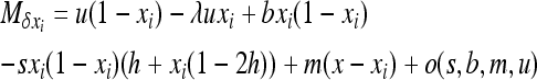
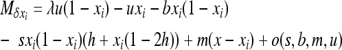
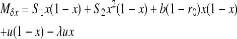
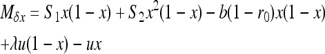
Throughout the article, I considered heterosis only as being caused by the masking of partially recessive deleterious alleles in hybrid individuals. As in Glémin (2010), I considered a single biallelic locus with weak (W = A or T) and strong (S = G or C) alleles. If the S (resp. W) allele is deleterious, the relative fitnesses of WW (resp. SS), WS, and SS (resp. WW) genotypes are 1, 1 − hs, and 1 − s, respectively, where s is the selection coefficient and h the dominance coefficient. The life cycle is as follows: N diploid adults produce gametes after conversion followed by mutation events. Heterozygote individuals produce S alleles with probability 1/2(1 + b) and W alleles with probability 1/2(1 − b), where b is the gBGC coefficient (disparity coefficient sensu Nagylaki 1983a). The W allele then mutates at rate u to the S allele. The reverse mutation occurs at rate v = λu. λ is the mutation bias from S to W alleles, which ranges from 2 to 4.5 in many different organisms (Lynch 2007). Fertilization occurs at random and it is followed by selection, migration, and regulation to N  individuals [“soft selection” model (e.g., Whitlock 2002; Roze and Rousset 2003)]. For clarity, hard selection is not investigated here but could be taken into account using Roze and Rousset's (2003) or Whitlock's (2002) framework (see also discussion). I assume that u and v are much smaller than selection and conversion coefficients (u, v ≪ s, hs, and b). For simplicity, I also assume that the gBGC  intensity is constant. However, strong gBGC events are thought to be associated with short-lived recombination hotspots, at least in humans (McVean et al. 2004; Myers et al. 2005). I thus implicitly assume that gBGC/selection dynamics are shorter than the recombination hotspot life span. The validity of this assumption is discussed in Glémin (2010).

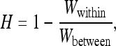
Heterosis can be defined as the increase in fitness of individuals derived from crosses between populations relative to individuals derived from crosses within a population,

(1)

where W_within is the average fitness of individuals produced by random mating within demes and W_between is the average fitness of individuals whose parents are sampled from different demes. Other authors have also defined W_between as the fitness of individuals whose parents are sampled from the whole metapopulation (Whitlock 2002; Roze and Rousset 2004, 2009). The first definition better matches experimental designs while the second one is more mathematically convenient. However, as the number of demes tends toward infinity, the two definitions become equivalent.

Wright's infinite island model with gBGC:

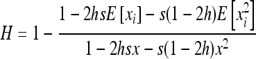
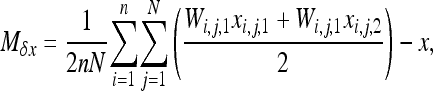
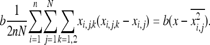
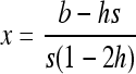
In the infinite island model, heterosis can be expressed as a function of deleterious allele frequencies as

(2)

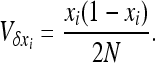
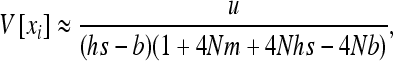
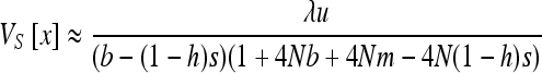
(e.g., Roze and Rousset 2004, 2009), where x_i is the local frequency of the deleterious allele in deme i, E denotes averaging over all demes, and x is the average frequency over the whole metapopulation. We thus have and (2) reduces to

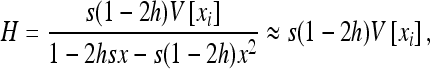(3)

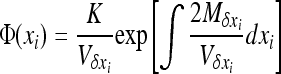
where V denotes the variance of allele frequencies over all demes. The right-hand term is an approximated expression for weak selection and/or for deleterious alleles maintained at low frequencies (e.g., Glémin et al. 2003; Roze and Rousset 2004, 2009). x_i and V[x_i] can be computed using Wright's distribution of allele frequencies in the infinite island model (Wright 1937), which gives the distribution of allele frequencies within a deme, assuming all demes are equivalent and migration is symmetrical, as

(4)

with

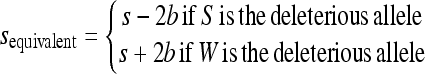
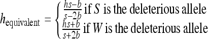
if S is the deleterious allele,

if W is the deleterious allele, and

This leads to

(5a)

if S is the deleterious allele and

(5b)

if W is the deleterious allele. is obtained by assuming that selection, gBGC, migration, and mutation are weak enough to neglect interaction terms between these elementary processes (without migration, see Equations 5a and 5b in Glémin 2010). K is an integration constant, ensuring that 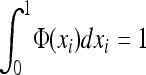, and x can be computed numerically by an iteration procedure until 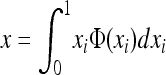(Barton and Rouhani 1993) and using the Kimura et al. (1963) quadrature method (for adaptation to gBGC and selection see Glémin 2010). This was done using a Mathematica script (Wolfram 1996) available on request. V[x] is then given by 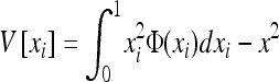. This approach is the same as in Whitlock et al. (2000), including gBGC in addition to selection. There is no general explicit analytical solution for (5a) and (5b); however, approximations can be obtained as developed below.

Analytical approximations:

Weak selection:

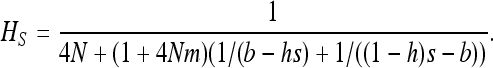
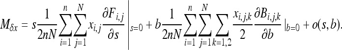
When selection is weak and migration not too small, we can use the approach developed by Roze and Rousset (2003, 2004). They showed that heterosis can also be expressed as

(6)

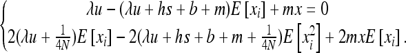
(Roze and Rousset 2004, 2009), where F is the probability of coalescence within the same deme of two genes sampled with replacement from the same deme, and it is equivalent to F_ST in the infinite neutral island model. x can then be computed using diffusion approximations according to Roze and Rousset (2003). Using the direct fitness method (Rousset and Billiard 2000), the infinitesimal expected change in allele frequency in the whole metapopulation is given by

(7a)

(appendix a) if S is the deleterious allele and by

(7b)

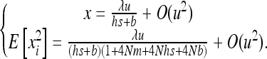
if W is the deleterious allele, with , , and . As I consider only the special case of the infinite island model, , and x can be simply obtained by solving .

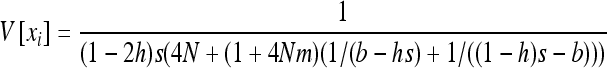
Strong selection:

When selection is strong and/or migration low, the previous method is not very accurate. When ∼Nhs > 5, the method developed by Glémin et al. (2003), adapted from Otha and Kimura's moment method (Ohta and Kimura 1969, 1971), can then be used instead. The aim is to obtain an analytical expression for V[x_i] to incorporate in Equation 3. Basically, the rationale is to obtain a set of linear equations as functions of moments of the distribution, Φ. Let be the infinitesimal expected change of allele frequency in deme i, be its variance, and be the covariance of the change between demes i and j. For any function f(x₁,…, x_i,…), Ohta and Kimura (1969, 1971) showed that

(8a)

which reduces to

(8b)

because (Glémin et al. 2003).

At equilibrium, . By choosing appropriate f functions, expressions can be obtained for each moment of Φ. However, this method leads to an infinite system of equations. To be solved, the system of recurrence equations must be closed, which can be done by linearizing (Glémin et al. 2003) or by arbitrarily assuming that moments vanish beyond a given order (Glémin 2005; Theodorou and Couvet 2006). Here, I used the linearization method (see appendix b). This assumes that selection is strong enough to maintain the average allele frequency at its deterministic equilibrium (as predicted by Glémin 2010). While this approximation for x is very rough, this leads to quite good approximations for the variance, V[x], i.e., the main determinant of heterosis (Glémin et al. 2003).

Multilocus predictions:

To assess the quantitative effect of gBGC, multilocus heterosis can be computed under the assumption of the multiplicative contribution to heterosis of all L loci throughout the genome. Assuming a fraction p of these loci are affected by gBGC, and a given distribution of fitness effects of mutations (DFEM), ψ, we have

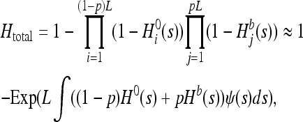(9)

where H⁰ and H^b denote heterosis without and with gBGC, respectively. Assuming half of deleterious mutations are S and the other half are W, H_total = (H_S + H_W)/2. I tested various more or less heterogenous gBGC distributions. Indeed, recombination and conversion are not distributed similarly in all organisms. For instance, recombination is probably not localized in hotspots in Caenorhabditis elegans (Rockman and Kruglyak 2009). I considered gBGC occurred in hotspots spanning p = 3% of the genome with b = 0.0002 on average [according to estimates in humans (Spencer et al. 2006)] or p = 5% and b = 0.0005. I also considered gBGC was homogeneously distributed over the whole genome (p = 100%) with b = 6.10⁻⁶ (that is, 3% × 0.0002) or restricted to very hot hotspots with b = 0.002 in frequency p = 0.3%. I assumed the DFEM was gamma distributed with mean s₀ and shape parameter α,

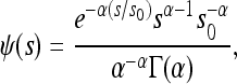(10)

where Γ is the gamma function (Abramowitz and Stegun 1970). I used s₀ = 0.0325 and α = 0.23 [according to estimates in humans (Eyre-Walker et al. 2006)]. Since heterosis strongly depends on dominance levels of mutations, which are poorly known, I explored different dominance levels. Equation 9 cannot be directly integrated using routine functions such as NIntegrate in Mathematica (Wolfram 1996) because the iteration procedure is needed for each s (see above). The gamma distribution (Equation 10) was thus discretized into 100 categories, according to Yang (1994).

RESULTS

Single-locus results and approximate solutions:

For weak selection and not too small migration, very good approximations are obtained by solving Equations 7a and 7b (see Figures 1–3). However, the analytical expressions are complicated and not given here. We can thus get more useful approximations in different conditions.

Figure 1.—

Heterosis as a function of s with and without gBGC. Circles were obtained by numerical integration of Equations 5: open circles, without gBGC; solid circles, with gBGC, b = 0.0002. Other parameters: N = 100, m = 0.01, u = 10⁻⁶, λ = 2, and h = 0.2. Solid lines show weak selection approximation, exact solutions of Equations 7. Dashed lines show strong selection approximations, Equations 12, 14, and 16. (A) W → S mutations; (B) S → W mutations.

Figure 3.—

Heterosis as a function of migration rate (m) with and without gBGC. Solid circles were obtained by numerical integration of Equations 5 and compared to exact solutions of Equations 7. Thick solid line, b = 0; solid line, b = 0.00005; long-dashed line, b = 0.0002; short-dashed line, b = 0.0004; dotted line, b = 0.0005. Other parameters: N = 100, u = 10⁻⁶, λ = 2, h = 0, and s = 0.001.

Figure 2.—

Heterosis as a function of gBGC intensity (b). Solid circles were obtained by numerical integration of Equations 5 and compared to exact solutions of Equations 7. Solid line, s = 0.001; dashed line, s = 0.01; dotted line, s = 0.05. Other parameters: N = 100, m = 0.01, u = 10⁻⁶, λ = 2, and h = 0.2.

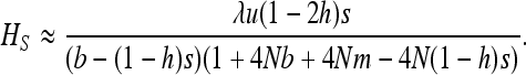
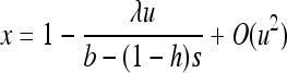
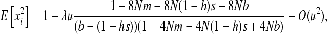
The case of W deleterious alleles is straightforward because selection and gBGC act in the same direction against W alleles. The deleterious allele is maintained at a lower frequency than under mutation/selection equilibrium, and the variance and heterosis are also reduced. For weak selection, neglecting back mutation and terms in x² and more in (7a), and assuming u ≪ s, b leads to

(11)

(see appendix a). For strong selection (see appendix b),

(12)

As expected, gBGC slightly reduces heterosis. When the S allele is deleterious, Glémin (2010) showed that the interaction between selection and gBGC leads to three selection regimes. If gBGC is weak relative to selection (b < hs), the deleterious S allele is maintained at low frequency, but slightly higher than at mutation/selection equilibrium, which leads to the same equations as (11) and (12), while replacing b by −b and λu by u. On the contrary, if gBGC is strong (b > (1 − h)s), the deleterious allele is close to fixation. For weak selection, linearizing (7b) in x around 1 and neglecting direct mutation leads to

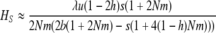(13)

(see appendix a). For strong selection (see appendix b),

(14)

Finally, if gBGC and selection are of similar intensity (hs < b < (1 − h)s), the two forces can maintain the deleterious allele at intermediate frequency. For weak selection, neglecting mutations and solving (7b) gives

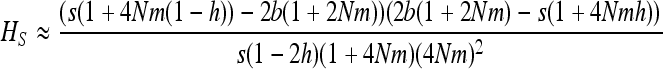(15)

(see appendix a). For strong selection (see appendix b),

(16)

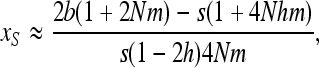
Note that the conditions for maintenance of the deleterious allele at intermediate frequency, and thus (15) being positive, are a bit more restrictive than in an unstructured population, , which vanish to the single-population conditions, hs < b < (1 − h)s, when Nm ≫ 1. This parallels the effect of inbreeding in single populations (Glémin 2010). Analytical approximations and numerical results (Figures 1 and 2) show that gBGC can strongly increase heterosis, mainly under the overdominant-like regime. Equations 15 and 16 also show that under the overdominant-like regime heterosis is mainly independent of mutation rates, contrary to the other regimes (Equations 11–14). At the genome scale, this means that if there are numerous such loci, heterosis can be high, even with low mutation rate. For other loci the total genomic mutation rate, not the number of loci, matters (i.e., few loci with high mutation rates are roughly equivalent to many loci with low mutation rates).

For both weak and strong selection, an analysis of Equations 15 and 16 shows that heterosis is maximal for b = s/2, that is, the gBGC value maximizing the load and inbreeding depression as well (Glémin 2010). For this parameter range, heterosis can be increased by a factor of ∼hs/4u compared with the case without gBGC (see appendixes a and b). This can be very high if the mutation rate is low, i.e., ∼10–1000. However, when gBGC is much higher than the selection, it reduces heterosis because it drives S deleterious alleles to fixation on the metapopulation scale (Figure 2). Conversely, for a given gBGC level, mutations maximizing heterosis are S mutations with effect , that is, mutations with effects between 2b and , or for fully recessive mutations (appendixes a and b). Mutations maximizing heterosis are thus mainly independent of the number of migrants, Nm, contrary to what was observed without gBGC (Whitlock et al. 2000).

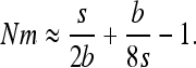
Another surprising consequence of the interaction of gBGC and selection is that heterosis can reach a local maximum for intermediate migrant numbers, especially for highly recessive W → S mutations. In the case of fully recessive alleles, this local maximum is reached for 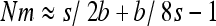(Figure 3 and appendix a). This can be explained because on one hand subdivision increases local drift, which increases heterosis, and on the other hand, subdivision increases local homozygosity, which reduces gBGC and thus heterosis. Because of these two opposing forces, maximum heterosis can thus be reached for intermediate levels of subdivision.

Quantitative patterns:

Single-locus analyses clearly showed that gBGC can affect the heterosis pattern, especially the contribution of different classes of mutations to heterosis. With gBGC, mutations contributing to heterosis are mainly restricted to those between b/(1 − h) and b/h, while the distribution is more homogeneous without gBGC and depends on the population size and migration (Figure 1). Moreover, assuming the DFEM follows a gamma distribution, W → S mutations of intermediate effect also contribute more than others, although they are not the most frequent. These mutations can contribute from a few to 10% of the total amount of heterosis while they represent only <1% of the total arising new mutations (Table 1). On the contrary, without gBGC, mutations with a very weak effect contribute the most to heterosis, simply because they are the most frequent.

TABLE 1.

Total quantitative effects of gBGC on heterosis and contribution of W → S mutations under the “overdominant-like” regime

		No gBGC	p = 1; b = 6.10−6	p = 0.03; b = 0.0002	p = 0.05; b = 0.0005	p = 0.003; b = 0.002
h = 0.1	Nm = 0.5	0.703	0.703a	0.708	0.726	0.711
			11/2.4b	7/0.2	26/0.3	8/0.03
	Nm = 1	0.576	0.575	0.581	0.604	0.585
			9/2.4	6/0.2	26/0.3	8/0.03
	Nm = 5	0.277	0.277	0.281	0.298	0.284
			5/2.4	5/0.2	22/0.3	7/0.03
h = 0.2	Nm = 0.5	0.520	0.519	0.523	0.54	0.526
			9/1.4	5/0.1	20/0.2	6/0.02
	Nm = 1	0.378	0.377	0.382	0.4	0.385
			7/1.4	5/0.1	21/0.2	6/0.02
	Nm = 5	0.137	0.137	0.139	0.149	0.141
			5/1.4	4/0.1	19/0.2	6/0.02
h = 0.3	Nm = 0.5	0.336	0.335	0.338	0.349	0.34
			8/0.8	4/0.06	14/0.1	4/0.01
	Nm = 1	0.221	0.22	0.223	0.233	0.224
			7/0.8	4/0.06	16/0.1	4/0.01
	Nm = 5	0.068	0.067	0.068	0.072	0.069
			6/0.8	4/0.06	17/0.1	4/0.01

^aTotal amount of heterosis: numerical integration of Equation 9 with u = 10⁻⁶, λ = 2, L = 10⁶, and N = 100. Parameters of the DFEM are given in the main text.

^bShilled entries show percentage of heterosis due to W → S mutations for which b/(1 − h) < s < b/h and percentage of such mutations in the whole mutation spectrum.

However, the total amount of heterosis is only slightly affected by gBGC, because it has opposite effects for different kinds of mutations. While it increases heterosis for rather strong S mutations (s > b/(1 − h)), it decreases it for weak ones (s < b/(1 − h)) and for all W mutations. Low gBGC, but widespread throughout the genome, has almost no effect. Only a rather high level of gBGC can significantly increase heterosis, mostly when deleterious mutations are highly recessive (Table 1).

DISCUSSION

Biased gene conversion can greatly affect the fate of selected alleles (Gutz and Leslie 1976; Lamb and Helmi 1982; Nagylaki 1983a,b; Bengtsson 1990). In several organisms, gBGC is a genome-wide biased gene conversion mechanism that can have quantitative fitness consequences. Recently, I showed that gBGC may strongly affect the mutation load, both qualitatively and quantitatively (Glémin 2010). Even rather weak gBGC restricted to a few genomic regions can create a substantial load by driving GC deleterious alleles to high frequency and fixation. I also showed that the interaction between selection and gBGC can generate an overdominant-like regime, maintaining recessive deleterious mutations at intermediate frequency for long periods of time, thus generating inbreeding depression. Here I investigated how gBGC could affect the fate of deleterious alleles in subdivided populations and thus another aspect of fitness, i.e., heterosis, which measures the increase in fitness due to crosses between demes relative to crosses within demes.

Contrary to its effect on the load, gBGC has only a very weak quantitative impact on heterosis, at least for levels in the range of what have been observed in a few species (Table 1). First, while heterosis is expected to be higher when local demes are small and isolated, gBGC intensity is reduced under these conditions because homozygosity is higher. Second, gBGC has an opposite effect on W and S deleterious mutations. However, its effect on S deleterious mutations is much stronger than its effect on W ones; on average, gBGC thus strongly increases the frequency of deleterious mutations and hence the load. However, heterosis depends on segregating mutations. Provided that b > hs, all weakly deleterious mutations affected by gBGC contribute to the load, while only those maintained at intermediate frequencies of ∼b/(1 − h) < s < b/h significantly increase heterosis. Weakly deleterious mutations fixed by gBGC increase the load but do not contribute to heterosis. The quantitative impact of gBGC is thus strongly dependent on the distribution of fitness and dominance effects of mutations. Numerical values explored in Table 1 suggest that in various contexts the quantitative effect of gBGC should be weak. However, a better characterization of these parameters is needed to evaluate the proportion of mutations submitted to the overdominant-like regime.

While gBGC should have a weak quantitative effect on heterosis, it may strongly affect its genetic basis. First, for a given gBGC level, S deleterious mutations corresponding to the overdominant-like regime contribute disproportionally to heterosis. For instance, using selection parameters from human data and several dominance levels, such mutations can cause a few to 10% of heterosis while representing only <1% of the whole spectrum of mutations (see Table 1 for several numerical examples). Interestingly, these mutations cause both heterosis and inbreeding depression (Glémin 2010). On the contrary, without gBGC, these two phenomena are expected to have a different basis, with heterosis being mainly caused by weakly deleterious mutations while inbreeding depression is mainly caused by strongly deleterious ones (Whitlock et al. 2000; Glémin et al. 2003). This variation in the genetic basis of heterosis may also depend on the degree of population structure, as gBGC may have a maximum effect for intermediate migrant numbers, Nm (Figure 3), and the range of mutations belonging to the overdominant-like regime depends on Nm (see Equation 15).

The genetic basis of heterosis has been debated for more than a century. These theoretical results suggest that gBGC should be taken into account as a potential additional factor, especially in species for which gBGC can be strong. This is typically the case for maize, probably the plant most studied for heterosis, and it belongs to the grass family in which gBGC is supposed to be strong (Glémin et al. 2006; Haudry et al. 2008; Escobar et al. 2010). Massive genomic data on maize are now available to study heterosis at the molecular level, both through crossing experiments (Swanson-Wagner et al. 2009) and through population genetics approaches (Gore et al. 2009). The results presented here lead to several predictions, which should now be testable on the basis of these new data. First, genes belonging to highly recombining regions should contribute disproportionally to heterosis compared to those in other genomic regions. This prediction is robust because such regions may have a higher local effective population size (Gordo and Charlesworth 2001) and thus contribute less to heterosis if gBGC is inactive. Second, W/S polymorphism should be involved more frequently than expected and the two alleles should segregate at intermediate frequencies, especially under the “overdominant-like” selection regime. However, it is worth noting that, contrary to their overdominant population behavior, such alleles should give clear dominance/recessive signatures when heterosis is estimated through cross-designs.

Here, I investigated only the case of soft selection. However, the conclusions should be very similar under hard selection. Using the hard selection model given by Roze and Rousset (2003), i.e., there is no local regulation before migration contrary to the life cycle studied here, the results are expected to be very close to those obtained under soft selection, except when deme sizes are very small, as shown by Roze and Rousset (2003, 2004). Whitlock (2002) initially proposed another model of hard selection where the contribution of each deme to the next generation is proportional to the mean relative fitness of the deme. Under this model, selection occurs between unrelated individuals (at the metapopulation scale) and it is thus stronger than under soft selection, where related individuals compete locally. Heterosis is thus expected to be lower; however, the effect of gBGC is similar. Indeed, this model is equivalent to a single inbreeding population, replacing F_IS by F_ST (Whitlock 2002), so that single-population results given in Glémin (2010) can be directly used (results not shown).

In summary, gBGC is likely a negligible process affecting the overall magnitude of heterosis in natural or breeding populations. However, these results strongly suggest that it should be taken into account when dissecting its genetic basis. To do so, quantification of the magnitude and distribution of gBGC throughout genomes in various organisms will be a critical issue for future studies.

APPENDIX A: APPROXIMATION FOR WEAK SELECTION

Derivation of Equations 7:

In the limit of weak selection and weak gBGC, the gBGC and selection model is equivalent to changing parameters as follows:

(A1)

(Glémin 2010). We can thus directly use these expressions in Equation 23 in Roze and Rousset (2003) to get Equations 7a and 7b. We can also derive Equations 7a and 7b by considering additively the effect of selection (Equation 23 in Roze and Rousset 2003) and gBGC as a form of genic selection (Equation 23 with h = and s = 2b in Roze and Rousset 2003).

Finally, a more complete derivation can also be obtained by modification of the equation of Roze and Rousset (2003) by the addition of gBGC. Here I present the case of S deleterious alleles. Consider the Wright island model with n demes of size N. The infinitesimal expected change in the deleterious allele frequency on the whole metapopulation, x, can be expressed as

(A2)

where W_i,j,k (k = 1, 2) is the fitness function defined at the gene lineage level, that is, the expected number of gene copies left by gene lineage k in individual j in population i. Similarly, x_i,j,k is the frequency of the deleterious allele in gene lineage k in individual j in population i. x_i,j,k = 0 or 1 and x_i,j = 0, , or 1. Note that according to this definition the total fitness of the population sums up to 2. One can write W_i,j,k as the product of a selection component, F_i,j(s) (equivalent to W_i,j in Roze and Rousset 2003), and a gBGC component, B_i,j,k:

Taylor's expansion of (A2) in s and b gives

(A3)

The first term, in s, is the same as that in Equation 13 in Roze and Rousset (2003) and leads to their Equation 23. The second term, in b, is expressed as

(A4)

The right-hand term is based on the fact that and 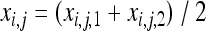. Roze and Rousset (2003) showed that (Equation 16) 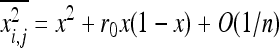, where r₀ is the probability of coalescence of two genes sampled with replacement from the same individual in a metapopulation with an infinite number of demes. Under panmixia, 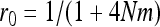. Equation A4 thus becomes 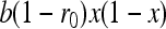, which is equivalent to the expected change in allele frequency under genic selection. These computations lead to Equations 7a and 7b.

Analysis of Equations 7:

For W deleterious mutations, linearizing (7a) in x near 0 and neglecting back mutation gives

(A5)

which leads to (11).

For S deleterious mutations with b < hs, linearizing (7b) in x near 0 and neglecting back mutation gives

(A6)

which leads to Equation 11 with the appropriate change of b by –b and λu by u.

For b > (1 − h)s, linearizing (7b) in x near 1 and neglecting direct mutations gives

(A7)

which leads to (13).

Finally, for the overdominant-like regime, hs < b < (1 − h)s, neglecting both direct and back mutations leads to

(A8)

which leads to (15).

Solving in b (for x_S given by Equation 15) shows that heterosis is maximal for b = s/2, for which , while for b = 0, heterosis is only . Under this condition, we thus have .

Solving (for x_S given by Equation 15) in s shows that mutations maximizing heterosis are S mutationswith . Finally, we can also show that heterosis can reach a local maximum for an intermediate number of migrants by solving 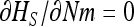in Nm, using Equation 15 for H_S, that is, considering only the overdominant-like selection regime. The full result is very substantial and not given here. Simple approximations can be obtained for fully recessive alleles. Noting β = b/s, Taylor expansion of the solution in β simply gives

APPENDIX B: APPROXIMATION FOR STRONG SELECTION

Using Equation 8b with appropriate f functions, one can get a set of equations of the moments of φ. To solve this system, must be linear in x_i (see Glémin et al. 2003). For W deleterious mutations, linearizing in x_i around 0 and neglecting back mutation give

(B1)

Using and in (8b) leads to

(B2)

Recalling that E[x_i] = x, the solution of (B2) is

(B3)

Since x is in O(u²), 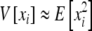, which can be inserted in (3) and gives (12).

Similarly, for S deleterious alleles, for gBGC weaker than selection, b < hs, linearizing in x_i around 0, neglecting back mutations, using the same f functions, and solving the system with the same approximations gives

(B4a)

and

(B4b)

which leads to (12) with the appropriate change of b by −b and λu by u.

For gBGC stronger than selection, b > (1 − h)s, linearizing in x_i around 1, neglecting direct mutations, using the same f functions, and solving the system leads to

(B5a)

and

(B5b)

which leads to

(B5c)

and to Equation 14.

Finally, for the overdominant-like regime, hs < b < (1 − h)s, one can linearize in x_i around the deterministic equilibrium, 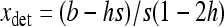(Glémin 2010), and neglect both direct and back mutations. Using the same f functions and solving the system leads to

(B6a)

and

(B6b)

which leads to

(B6c)

and to Equation 16.

References

- Abramowitz, M., and I. A. Stegun, 1970. Handbook of Mathematical Functions. Dover, New York.
- Barton, N. H., and S. Rouhani, 1993. Adaptation and the ‘shifting balance’. Genet. Res. 61 57–74. [Google Scholar]
- Bengtsson, B. O., 1990. The effect of biased conversion on the mutation load. Genet. Res. 55 183–187. [DOI] [PubMed] [Google Scholar]
- Davenport, C. B., 1908. Degeneration, albinism and inbreeding. Science 28 454–455. [DOI] [PubMed] [Google Scholar]
- Duret, L., and N. Galtier, 2009. Biased gene conversion and the evolution of mammalian genomic landscapes. Annu. Rev. Genomics Hum. Genet. 10 285–311. [DOI] [PubMed] [Google Scholar]
- Duvick, D. N., 2001. Biotechnology in the 1930s: the development of hybrid maize. Nat. Rev. Genet. 2 69–74. [DOI] [PubMed] [Google Scholar]
- East, E. M., 1908. Inbreeding in corn. Conn. Agric. Exp. Stn. Rep., 419–428.
- Escobar, J. S., A. Nicot and P. David, 2008. The different sources of variation in inbreeding depression, heterosis and outbreeding depression in a metapopulation of Physa acuta. Genetics 180 1593–1608. [DOI] [PMC free article] [PubMed] [Google Scholar]
- Escobar, J. S., A. Cenci, J. Bolognini, A. Haudry, S. Laurent et al., 2010. An integrative test of the dead-end hypothesis of selfing evolution in Triticeae (Poaceae). Evolution 64 2855–2872. [DOI] [PubMed] [Google Scholar]
- Eyre-Walker, A., M. Woolfit and T. Phelps, 2006. The distribution of fitness effects of new deleterious amino acid mutations in humans. Genetics 173 891–900. [DOI] [PMC free article] [PubMed] [Google Scholar]
- Facon, B., P. Jarne, J. P. Pointier and P. David, 2005. Hybridization and invasiveness in the freshwater snail Melanoides tuberculata: hybrid vigour is more important than increase in genetic variance. J. Evol. Biol. 18 524–535. [DOI] [PubMed] [Google Scholar]
- Galtier, N., and L. Duret, 2007. Adaptation or biased gene conversion? Extending the null hypothesis of molecular evolution. Trends Genet. 23 273–277. [DOI] [PubMed] [Google Scholar]
- Galtier, N., L. Duret, S. Glémin and V. Ranwez, 2009. GC-biased gene conversion promotes the fixation of deleterious amino acid changes in primates. Trends Genet. 25 1–5. [DOI] [PubMed] [Google Scholar]
- Glémin, S., 2005. Lethals in subdivided populations. Genet. Res. 86 41–51. [DOI] [PubMed] [Google Scholar]
- Glémin, S., 2010. Surprising fitness consequences of GC-biased gene conversion: I. Mutation load and inbreeding depression. Genetics 185 939–959. [DOI] [PMC free article] [PubMed] [Google Scholar]
- Glémin, S., J. Ronfort and T. Bataillon, 2003. Patterns of inbreeding depression and architecture of the load in subdivided populations. Genetics 165 2193–2212. [DOI] [PMC free article] [PubMed] [Google Scholar]
- Glémin, S., E. Bazin and D. Charlesworth, 2006. Impact of mating systems on patterns of sequence polymorphism in flowering plants. Proc. R. Soc. Lond. B 273 3011–3019. [DOI] [PMC free article] [PubMed] [Google Scholar]
- Gordo, I., and B. Charlesworth, 2001. Genetic linkage and molecular evolution. Curr. Biol. 11 R684–R686. [DOI] [PubMed] [Google Scholar]
- Gore, M. A., J. M. Chia, R. J. Elshire, Q. Sun, E. S. Ersoz et al., 2009. A first-generation haplotype map of maize. Science 326 1115–1117. [DOI] [PubMed] [Google Scholar]
- Guillaume, F., and N. Perrin, 2006. Joint evolution of dispersal and inbreeding load. Genetics 173 497–509. [DOI] [PMC free article] [PubMed] [Google Scholar]
- Gutz, H., and J. F. Leslie, 1976. Gene conversion: a hitherto overlooked parameter in population genetics. Genetics 83 861–866. [DOI] [PMC free article] [PubMed] [Google Scholar]
- Haudry, A., A. Cenci, C. Guilhaumon, E. Paux, S. Poirier et al., 2008. Mating system and recombination affect molecular evolution in four Triticeae species. Genet. Res. 90 97–109. [DOI] [PubMed] [Google Scholar]
- Hogg, J. T., S. H. Forbes, B. M. Steele and G. Luikart, 2006. Genetic rescue of an insular population of large mammals. Proc. R. Soc. B Biol. Sci. 273 1491–1499. [DOI] [PMC free article] [PubMed] [Google Scholar]
- Hua, J. P., Y. Z. Xing, W. R. Wu, C. G. Xu, X. L. Sun et al., 2003. Single-locus heterotic effects and dominance by dominance interactions can adequately explain the genetic basis of heterosis in an elite rice hybrid. Proc. Natl. Acad. Sci. USA 100 2574–2579. [DOI] [PMC free article] [PubMed] [Google Scholar]
- Kimura, M., T. Maruyama and J. F. Crow, 1963. The mutation load in small populations. Genetics 48 1303–1312. [DOI] [PMC free article] [PubMed] [Google Scholar]
- Lamb, B. C., and S. Helmi, 1982. The extent to which gene conversion can change allele frequencies in populations. Genet. Res. 39 199–217. [Google Scholar]
- Lynch, M., 2007. The Origin of Genome Architecture. Sinauer Associates, Sunderland, MA.
- Marais, G., 2003. Biased gene conversion: implications for genome and sex evolution. Trends Genet. 19 330–338. [DOI] [PubMed] [Google Scholar]
- McVean, G. A., S. R. Myers, S. Hunt, P. Deloukas, D. R. Bentley et al., 2004. The fine-scale structure of recombination rate variation in the human genome. Science 304 581–584. [DOI] [PubMed] [Google Scholar]
- Myers, S., L. Bottolo, C. Freeman, G. McVean and P. Donnelly, 2005. A fine-scale map of recombination rates and hotspots across the human genome. Science 310 321–324. [DOI] [PubMed] [Google Scholar]
- Nagylaki, T., 1983. a Evolution of a finite population under gene conversion. Proc. Natl. Acad. Sci. USA 80 6278–6281. [DOI] [PMC free article] [PubMed] [Google Scholar]
- Nagylaki, T., 1983. b Evolution of a large population under gene conversion. Proc. Natl. Acad. Sci. USA 80 5941–5945. [DOI] [PMC free article] [PubMed] [Google Scholar]
- Ohta, T., and M. Kimura, 1969. Linkage disequilibrium at steady state determined by random genetic drift and recurrent mutation. Genetics 63 229–238. [DOI] [PMC free article] [PubMed] [Google Scholar]
- Ohta, T., and M. Kimura, 1971. Linkage disequilibrium between two segregating nucleotide sites under the steady flux of mutations in a finite population. Genetics 68 571–580. [DOI] [PMC free article] [PubMed] [Google Scholar]
- Reif, J. C., A. E. Melchinger, X. C. Xia, M. L. Warburton, D. A. Hoisington et al., 2003. Genetic distance based on simple sequence repeats and heterosis in tropical maize populations. Crop Sci. 43 1275–1282. [Google Scholar]
- Richards, C. M., 2000. Inbreeding depression and genetic rescue in a plant metapopulation. Am. Nat. 155 283–294. [DOI] [PubMed] [Google Scholar]
- Rockman, M. V., and L. Kruglyak, 2009. Recombinational landscape and population genomics of Caenorhabditis elegans. PLoS Genet. 5 e1000419. [DOI] [PMC free article] [PubMed] [Google Scholar]
- Ronfort, J., and D. Couvet, 1995. A stochastic model of selection on selfing rates in structured populations. Genet. Res. 65 209–222. [Google Scholar]
- Rousset, F., and S. Billiard, 2000. A theoretical basis for measures of kin selection in subdivided populations: finite populations and localized dispersal. J. Evol. Biol. 13 814–825. [Google Scholar]
- Roze, D., and F. Rousset, 2003. Selection and drift in subdivided populations: a straightforward method for deriving diffusion approximations and applications involving dominance, selfing and local extinctions. Genetics 165 2153–2166. [DOI] [PMC free article] [PubMed] [Google Scholar]
- Roze, D., and F. Rousset, 2004. Joint effects of self-fertilization and population structure on mutation load, inbreeding depression and heterosis. Genetics 167 1001–1015. [DOI] [PMC free article] [PubMed] [Google Scholar]
- Roze, D., and F. Rousset, 2009. Strong effects of heterosis on the evolution of dispersal rates. J. Evol. Biol. 22 1221–1233. [DOI] [PubMed] [Google Scholar]
- Semel, Y., J. Nissenbaum, N. Menda, M. Zinder, U. Krieger et al., 2006. Overdominant quantitative trait loci for yield and fitness in tomato. Proc. Natl. Acad. Sci. USA 103 12981–12986. [DOI] [PMC free article] [PubMed] [Google Scholar]
- Shull, G. H., 1911. The genotypes of maize. Am. Nat. 45 234–252. [Google Scholar]
- Shull, G. H., 1914. Duplicate genes for capsule form in Bursa bursa-pastoris. Z. Ind. Abstr. Vererb. 12 97–149. [Google Scholar]
- Spencer, C. C., P. Deloukas, S. Hunt, J. Mullikin, S. Myers et al., 2006. The influence of recombination on human genetic diversity. PLoS Genet. 2 e148. [DOI] [PMC free article] [PubMed] [Google Scholar]
- Swanson-Wagner, R. A., R. DeCook, Y. Jia, T. Bancroft, T. M. Ji et al., 2009. Paternal dominance of trans-eQTL influences gene expression patterns in maize hybrids. Science 326 1118–1120. [DOI] [PubMed] [Google Scholar]
- Theodorou, K., and D. Couvet, 2002. Inbreeding depression and heterosis in a subdivided population: influence of the mating system. Genet. Res. 80 107–116. [DOI] [PubMed] [Google Scholar]
- Theodorou, K., and D. Couvet, 2006. Genetic load in subdivided populations: interactions between the migration rate, the size and the number of subpopulations. Heredity 96 69–78. [DOI] [PubMed] [Google Scholar]
- Whitlock, M. C., 2002. Selection, load, and inbreeding depression in a large metapopulation. Genetics 160 1191–1202. [DOI] [PMC free article] [PubMed] [Google Scholar]
- Whitlock, M. C., P. K. Ingvarsson and T. Hatfield, 2000. Local drift load and the heterosis of interconnected populations. Heredity 84 452–457. [DOI] [PubMed] [Google Scholar]
- Willi, Y., and M. Fischer, 2005. Genetic rescue in interconnected populations of small and large size of the self-incompatible Ranunculus reptans. Heredity 95 437–443. [DOI] [PubMed] [Google Scholar]
- Willi, Y., M. Van Kleunen, S. Dietrich and M. Fischer, 2007. Genetic rescue persists beyond first-generation outbreeding in small populations of a rare plant. Proc. R. Soc. B Biol. Sci. 274 2357–2364. [DOI] [PMC free article] [PubMed] [Google Scholar]
- Wolfram, S., 1996. The Mathematica Book. Cambridge University Press, Cambridge, UK.
- Wright, S., 1937. The distribution of gene frequencies in populations. Proc. Natl. Acad. Sci. USA 23 307–320. [DOI] [PMC free article] [PubMed] [Google Scholar]
- Yang, Z., 1994. Estimating the pattern of nucleotide substitution. J. Mol. Evol. 39 105–111. [DOI] [PubMed] [Google Scholar]
- Yu, S. B., J. X. Li, Y. F. Tan, Y. J. Gao, X. H. Li et al., 1997. Importance of epistasis as the genetic basis of heterosis in an elite rice hybrid. Proc. Natl. Acad. Sci. USA 94 9226–9231. [DOI] [PMC free article] [PubMed] [Google Scholar]