A Simplified Mass-Transfer Model for Visual Pigments in Amphibian Retinal-Cone Outer Segments

Abstract

When radiolabeled precursors and autoradiography are used to investigate turnover of protein components in photoreceptive cone outer segments (COSs), the labeled components—primarily visual pigment molecules (opsins)—are diffusely distributed along the COS. To further assess this COS labeling pattern, we derive a simplified mass-transfer model for quantifying the contributions of advective and diffusive mechanisms to the distribution of opsins within COSs of the frog retina. Two opsin-containing regions of the COS are evaluated: the core axial array of disks and the plasmalemma. Numerical solutions of the mass-transfer model indicate three distinct stages of system evolution. In the first stage, plasmalemma diffusion is dominant. In the second stage, the plasmalemma density reaches a metastable state and transfer between the plasmalemma and disk region occurs, which is followed by an increase in density that is qualitatively similar for both regions. The final stage consists of both regions slowly evolving to the steady-state solution. Our results indicate that autoradiographic and cognate approaches for tracking labeled opsins in the COS cannot be effective methodologies for assessing new disk formation at the base of the COS.

Introduction

In the vertebrate eye, visual processes are initiated by the absorption of photons within specialized photoreceptor cells (rods and/or cones) of the retina (1). Cone cells generally subserve high-acuity color vision under conditions of high luminance (e.g., daylight conditions), whereas rod cells generally subserve low-acuity gray-level vision under conditions of low luminance (e.g., from dusk to dawn) (2). In frogs, rods consist of ∼58% of the receptor population and cones make up the other 42% (3). A light-absorbing organelle, called an outer segment (see Fig. 1), is located at the apical end of each photoreceptor cell and consists of an extended array of oriented, densely packed, paired lamellar membrane elements, called disks, that contain light-absorbing photopigment molecules. Each photopigment molecule has two basic components: an oriented, transmembrane glycoprotein called an opsin (∼38 kDa molecular mass), and a small, light-absorbing, vitamin-A-based chromophore (e.g., 11-cis-retinal, 284.44 Da molecular mass) that binds to the opsin in a stereospecific manner. The overall effect of these structural arrangements is to enhance the directional sensitivity of the outer segment for absorbing and detecting photons.

Figure 1.

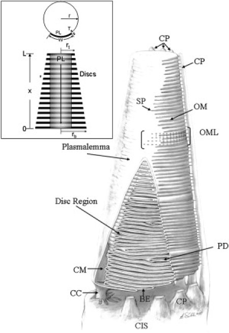
Three-dimensional rendering of COS geometry (conical frustum). This fully continuous system of membranes is divided into two main regions: a central stack of paired lamellar membrane units called disks, and a plasmalemma sheath that partially encloses the disks along one side. The two membranes of each disk are continuous along the closed margin (CM) segment of the disk perimeter; each disk is continuous with the two adjacent disks via the open margin (OM) segments of the perimeter. All four membrane domains are continuous at saddle points (SP), located at the junction of the plasmalemma with open margin segments. Each disk is associated with two saddle points. (The second set of saddle points would be located on the far side of the figure, not visible in this drawing) The COS is continuous with the CIS via the narrow connecting cilium (CC). From multiple points around the perimeter of the CIS, microvillus-like processes (calycal processes (CP)) project distally along the surface of the COS. The OM segments of the disk perimeters are interconnected by a two-dimensional lattice of components (5,21), the radial components of which connect to the CPs. A short stretch of open margin lattice (OML) is indicated. Developing disk precursors (basal evaginations (BE)) are indicated along the base of the COS. Within the disk stack, disks of smaller size (partial disk (PD)) are also present. The space between the base of the COS and the apical surface of the CIS is enlarged for visibility (these two surfaces are normally immediately adjacent to each other). Drawing by Dr. Bradley R. Smith. (Inset) The disk region modeled as a porous medium, with mass transport allowed within individual disks but not permitted axially between adjacent disks. For the membrane recycling component of the model, advective mass flow occurs radially from the disks to the plasmalemma; advective flow within the plasmalemma is directed basally. Diffusion of labeled opsin begins at the base of the COS and proceeds axially, with free diffusion allowed between disk and plasmalemma domains.

Much effort has been devoted to understanding the processes of synthesis, assembly, and turnover of outer-segment components, as well as the dynamics of photopigment movement and diffusion within these multilamellar membrane systems. Many fundamental aspects of the anatomy and physiology of vertebrate visual systems have derived from research on frogs (3), which is one of the reasons that frog cone outer segments (COSs) are the focus of this work. Much of our current understanding is derived from analyses of rod-cell outer segments (ROSs); the corresponding processes in COSs are less well understood, especially in the conically shaped COSs of lower vertebrates. In ROSs, new disks are formed in the basal region of the outer segment. Initially, the basal lamellae appear as small evaginations of the ROS plasmalemma from the medial surface of the connecting cilium, and are analogous to the evagination profiles observed in the basal COS (4). In ROSs, these evaginations expand in diameter until they approximate the diameter of the adjacent rod inner segment (RIS) and are progressively restructured along their margins into bimembranous disks. Eventually, the final link of continuity between the disk and the plasmalemma is lost through membrane fusion, and the disk becomes an independent unit (flattened membranous vesicle) sequestered within the surrounding plasmalemma (4,5). The basal lamellae of COSs resemble the transient basal evaginations of ROSs. The COS lamellae basically retain this initial topology along the length of the COS and display membrane continuity with the plasmalemma at highly curved growth points or saddle points (2,4,5).

The axial array of COS disks also displays a well-defined, truncated conical geometry (conical frustum), in contrast to the typically cylindrical geometry of ROSs. A drawing of the COS structure is shown in Fig. 1. Fig. 2 is an electron microscope autoradiogram of an ROS and a COS with the locations of labeled proteins indicated by the small silver grains. Fig. 3 shows the idealized COS used for our mass-transfer model. This conically tapered COS is consistent with micrographs reported in the literature (2,6–11). In this article, we explore a combined diffusion-advection model for integrating dynamical elements of new disk formation, apical disk displacement, opsin diffusion, and advective recycling of membrane components (opsins and lipids) within the COS.

Figure 2.

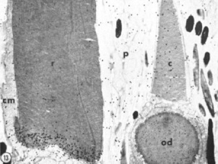
Labeling pattern of a ROS (r) and COS (c) 1 day after injection of labeled amino acids. Electron microscope autoradiogram, ×9600, showing the ciliary matrix (cm), oil droplet (od), and pigment epithelial process (p). Reprinted from Fig. 13 of Bok and Young (10), with permission from Elsevier.

Figure 3.

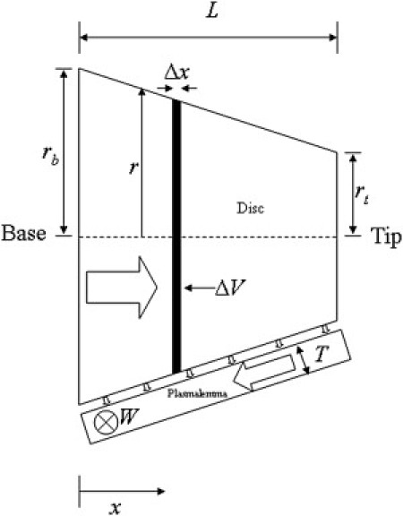
Idealized COS model geometry. The geometric symbols are defined in Table 1. Block arrows indicate direction of advective mass transport.

Autoradiography has provided the foundation for our current understanding of outer segment renewal in ROSs. When live animals are injected with radioactive amino acids or glycoprotein-precursor sugars to label opsins (and other proteins), and subsequently followed by autoradiography, radiolabeling is initially observed within the RIS, in the region of the rough endoplasmic reticulum (myoid) (12). With increasing time from injection, label moves through the Golgi zone and shifts progressively to the apex of the inner segment, near the periciliary ridge complex and the connecting cilium, and later still to the membranous lamellae of the basal ROS, where label accumulates predominantly over a basal group of developing disks (Fig. 2). When animals are examined at later time points, these labeled disks are observed at progressively greater distances from the base of the ROS. Eventually, the band of labeled disks reaches the tip of the ROS, where it is then shed, phagocytized and degraded by cells of the overlying retinal pigment epithelium. Thus, the opsins in ROS disks have a well-defined spatial pattern of turnover. Throughout apical displacement, disks typically retain the diameter established initially near the base of the ROS, thereby establishing the cylindrical geometry of the ROS.

Opsin turnover processes in COSs are less well understood. For example, frog COSs (Rana species) show no corresponding bands of radiolabeled disks (11,12), although in later work, Eckmiller (13) might have detected a small, transient increase in basal COS labeling without definitive banding in Xenopus. In a two-compartment model of mammalian COS labeling using ³H-fucose as the glycoprotein precursor, Anderson et al. (14) demonstrated increased labeling of the basal compartment up to 12 h after fucose injection. ROS-like banding was not observed in these COSs, which are much closer to ROSs in geometry and membrane topology. Like rod cells, cone cells display initial labeling of the rough endoplasmic reticulum and Golgi apparatus within the cone inner segment (CIS), but this initial labeling pattern is not followed by the labeling of membranous lamellae near the base of the COS or by the formation of a labeled band of lamellae that advances toward the COS apex. Instead, label appears to become distributed randomly throughout the length of the COS (Fig. 2). Thus, an early idea was that COS components may be renewed by a molecular replacement mechanism, and/or subject to diffusion throughout most of the COS membrane system via the structural continuity of COS membrane domains. It was later shown that groups of disks are shed from the tips of COSs and phagocytized by the retinal pigment epithelium in a manner analogous to that observed in ROSs (15). Thus, to maintain average COS length and geometry, tip shedding must be balanced by new disk formation. Disk formation appears to occur principally at the base of the COS, incorporating components available in the region of the connecting cilium. Eckmiller (6,16,17) has also suggested that a separate mechanism of disk formation, termed distal invagination, might occur in more apically located regions of the COS, based upon the presence of partial disk profiles and light-cycle-dependent changes in their axial distribution. Whether these profiles represent new disk formation or disk resorption (5) remains to be determined, and they are excluded from the analysis presented here.

An additional approach to interpreting these autoradiographic and electron microscopic results derives from considering the two dominant structural features of COS disks: 1), the continuity of disks with the plasmalemma at saddle points, and the continuity of adjacent disks along their margin segments; and 2), the regular conical geometry of the outer segment. As disks advance toward the tip of the COS, each disk must decrease in both area and perimeter to maintain the overall conical geometry. The likely points for mass transfer from each disk are the two saddle points that provide membrane continuity between each disk and the plasmalemma. Thus, if newly synthesized membrane components are delivered via the connecting cilium to the base of the COS for new disk assembly, then apical displacement of the stack of previously formed disks might lead to the transfer and incorporation of older disk membrane components into newly forming disks via intermediate transit along the plasmalemmal shaft of the COS. We call this transfer process recycling. This concept has been introduced briefly in previous work (5,8,9) and will be fully developed in a companion article (Corless, personal communication), so only a summary is included here.

Given the geometry of a frog COS (length, basal and apical diameters, and number and dimensions of disks), the addition of a new basal disk of area A would be associated with a reduction in total membrane area of the older disks by ∼0.88A (using data from Table 1, 6-h time point). Thus, ∼88% of the membrane components needed to form a new basal disk might be derived from preexisting disks, and only ∼12% from newly synthesized components. Such a mechanism would predict about an eightfold dilution of labeled photopigment molecules within a new basal COS disk. Axial diffusion during new disk formation might further dilute the labeling of a new basal disk.

Table 1.

Structural and physiological parameters used in model calculations

Parameter	Symbol	Value	Table S1 footnote
Mass diffusion coefficient	D	0.5 μm2/s	1
Disk base radius	rb	2.1 μm	2
Disk displacement velocity	u1	0.0001041 μm/s	3
Nonvoid fraction	ϕ	0.43	4
Plasmalemma thickness	T	0.0075 μm	4
Plasmalemma width	W	2.1 μm	5
COS length at light onset	L1	5.92 μm	3 (n = 171)
Disk tip radius at light onset	rt1	1.110 μm	3
COS length 6 h after light onset	L2	8.17 μm	3 (n = 236)
Disk tip radius 6 h after light onset	rt2	0.734 μm	3
COS length 10 h after light onset	L3	9.65 μm	3 (n = 279)
Disk tip radius 10 h after light onset	rt3	0.485 μm	3

A full interpretation of autoradiographic data from COSs would take into account the labeling of soluble proteins as well as membrane proteins (both integral and peripheral). This model is limited by available data and only addresses the membrane phase, focusing on opsins—integral transmembrane proteins that constitute the major protein species (∼70%) within outer segments, and thus will dominate the autoradiographic data. Radiolabeled sugar precursors (e.g., fucose) (14,18) can distinguish some transmembrane proteins (including opsins) from soluble proteins. Future work in COSs, similar to that conducted by Calvert et al. (19) using a diffusible soluble protein in ROSs, will be needed to explore the diffusion characteristics of the major soluble and membrane-associated proteins present within the COSs.

Although diffusion of radiolabeled components within the membrane phase has reasonably been invoked to explain qualitatively the diffuse axial labeling pattern and lack of banding in COSs, there is no systematic model for assessing these patterns quantitatively or for relating them to new disk formation. Thus, our current goals in developing such a model are severalfold:

• 1.To develop an initial 1-D model for the axial diffusion of labeled membrane components transferred to the COS from the CIS via the connecting cilium.
• 2.To model the effects of recycling of disk membrane components on axial diffusion within the COS.
• 3.To understand how axial diffusion and recycling can limit our ability to distinguish the basal site of insertion of labeled membrane components from the site of new disk formation.
• 4.To suggest additional approaches for investigating membrane dynamics, turnover, and renewal within the COS.

Mass transfer between the disk and plasmalemma, as well as mass transfer within the plasmalemma, will be the primary focus of this work. We assume that no advective or diffusional transfer of membrane components occurs directly between adjacent COS disks: all exchanges involve intermediate transfers to the plasmalemma. Structural data strongly suggest that the internal components of closed margin segments would present a barrier to the diffusion of opsins around these regions (20,21), and there is no evidence for a resident population of opsins within these domains (22,23), as judged from comparable ROS structural and labeling data. Open margin segments of disk perimeters display a two-dimensional lattice of components (Fig. 1) that are also positioned to impede or block opsin transit around these high-curvature domains (5,23). Bleaching-recovery studies indicate that the principal route for axial diffusion of opsins among disks is via the plasmalemma: disk to plasmalemma to disk (24–26), as discussed in Corless et al. (22). There is no experimental evidence for direct disk-to-disk transfers of opsins in COSs, although such routes remain a possibility. In our model, we assume that the density profile in both the plasmalemma and disk region is one-dimensional, analogous to heat transfer from fins with small Biot numbers. An additional goal of our model is to treat the disk region as a continuum. The remainder of this work is arranged in several sections. First, the descriptive partial differential equations (PDEs) for the radiolabeled protein density in the disk and plasmalemma regions are derived. The descriptive equations are nondimensionalized, and scaling arguments are applied. A brief discussion of the numerical method for solving the system equations is next, followed by the numerical results and their interpretation.

Materials and Methods

Derivation of radiolabeled opsin density model

In this section, we derive two simple coupled PDEs that give the density of radiolabeled opsins (hereafter referred to as label) in the disk and in the plasmalemma. The density of label in the disk and plasmalemma regions is denoted by numbers 1 and 2, respectively. In deriving this expression, the assumption is made that the density in the disk region may be accurately represented as a continuous function, analogous to a passive scalar quantity in a porous medium.

The disk region is modeled as a right circular conical frustum of height L, base radius r_b, and tip radius r_t. The plasmalemma is modeled as a rectangular duct with a cross sectional area of width W and thickness T. The plasmalemma is oriented in the axial direction external to the disk region. Fig. 3 shows the model geometry and reference coordinate system.

To formulate the model, we start with the COS geometry defined in Fig. 3 and the measured structural and physiological parameters for frog and amphibian COSs listed in Table 1. These parameter values were selected as reasonable and reflective of available data. Also, the process of nondimensionalizing the equations allows for the solution to describe a wide range of parameter values.

Before deriving these two equations, it is necessary to derive an equation for the disk-to-plasmalemma velocity and for the material velocity in the plasmalemma. The Supporting Material contains this derivation and a list of the physical meaning of each symbol; the final results for the disk-to-plasmalemma velocity, v, and the plasmalemma velocity, u₂ (Eq. S5 and Eq. S9 in the Supporting Material), are repeated here:

$$\begin{array}{l}v=\frac{2\pi \varphi u_1\left(r_t-r_b\right)}{LW}\left[r_b+\frac{x}{L}\left(r_t-r_b\right)\right]\hfill \\ u_2=-\frac{\pi \varphi u_1\left(r_t-r_b\right)}{LWT}\left[2r_{b}x+\frac{x^2}{L}\left(r_t-r_b\right)-L\left(r_t+r_b\right)\right]\hfill \end{array}.$$ (1)

A control volume is used for derivation of the mass balance equations (Fig. 4). The prime notation indicates species (radiolabeled opsin) velocity; e.g., $u_2^{\prime }$ is the species velocity in the plasmalemma, whereas u₂ is the bulk velocity. Assuming that the control volume length, Δx, is small, we can retain only the first term of the Taylor series expansion of the product of the flux and cross-sectional area and write for the plasmalemma label density, ρ₂,

$$\begin{array}{l}\frac{\partial {\rho }_2}{\partial t}WT\Delta x=NW\Delta x+WT{\rho }_2{u}_2^{\prime }-WT\left({\rho }_2{u}_2^{\prime }+\frac{\partial \left({\rho }_2{u}_2^{\prime }\right)}{\partial x}\Delta x\right)\to \hfill \\ T\frac{\partial {\rho }_2}{\partial t}=N-T\frac{\partial \left({\rho }_2{u}_2^{\prime }\right)}{\partial x}\hfill \end{array}.$$ (2)

In the above expression, N represents the flux from the disk to the plasmalemma and is defined as positive when mass is flowing from the disk into the plasmalemma. Next, Fick's Law is applied, which relates the species velocity to the bulk velocity via the introduction of a mass diffusivity term:

$${\rho }_2{u}_2^{\prime }=j_2+{\rho }_2{u}_2=-D\frac{\partial {\rho }_2}{\partial x}+{\rho }_2{u}_2.$$ (3)

In this expression, j₂ is the diffusion velocity and D is the constant diffusion coefficient. Next, using Eq. 3, we eliminate the product ${\rho }_2{u}_2^{\prime }$ in Eq. 2 to obtain:

$$T\frac{\partial {\rho }_2}{\partial t}=N-T\frac{\partial \left(-D\frac{\partial {\rho }_2}{\partial x}+{\rho }_2{u}_2\right)}{\partial x}=N+TD\frac{{\partial }^2{\rho }_2}{\partial x^2}-T\frac{\partial \left({\rho }_2{u}_2\right)}{\partial x}.$$ (4)

Figure 4.

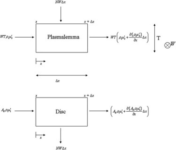
Plasmalemma control volume (upper) and disk control volume (lower).

We now consider N, which is the species flux from the disk region into the plasmalemma. An issue arises in that the diffusion constant, D, is no longer defined for the interface between the disk and plasmalemma regions, so we use a mass-transfer coefficient (h_m). h_m is defined as the ratio between the flux and the difference in concentration at an interface. Experimental data are usually used to assess the value of h_m, although scaling arguments may be used as well. (See Truskey et al. (27) for a more detailed discussion of the mass transfer coefficient.) For the assumption of a one-dimensional density distribution (e.g., Eq. 11) to be valid, the Biot number, Bi = h_mr/D, must be much less than 1. Therefore, the gradient of label along the plasmalemma must be small when compared to the difference in label concentration between the plasmalemma and adjacent disk. Although experimental values for r and D can be assigned (Table 1), the value of h_m has not been measured. If Bi were vanishingly small, we would expect to see axial banding within the COS, which is not the case: experimental data show only diffuse labeling along the COS. Thus, h_m has a finite value. In the Supporting Material, we estimate the value of h_m based upon the labeled-species flux due to diffusion and the best values for the axial disk repeat period (d) and the size and shape of the saddle point. These estimates fall in the range of h_m = 0.0162–0.02523 μm/s. The actual value of h_m remains to be determined experimentally.

Another issue that must be dealt with is the fact that the density of label in the disk area is a bulk (or average) density. Since the disk area has a nonvoid fraction of ϕ, the disk region label density ρ₁ must be scaled by this factor. We assume that the nonvoid fraction ϕ is constant along the COS (see footnote 4 for Table S1, in the Supporting Material). The species flux term becomes

$$N=h_m\left(\frac{{\rho }_1}{\varphi }-{\rho }_2\right)-\frac{{\rho }_{1}v}{\varphi }.$$ (5)

The negative sign in front of the ${\rho }_{1}v/\varphi$ term is necessary to satisfy the condition that the flux is positive when mass is flowing from the disk to the plasmalemma (v is the linear velocity of components flowing from the disk to the plasmalemma and is negative across the domain). Substituting Eq. 5 into Eq. 4 yields the PDE for the label density in the plasmalemma, ρ₂:

$$T\frac{\partial {\rho }_2}{\partial t}=h_m\left(\frac{{\rho }_1}{\varphi }-{\rho }_2\right)-\frac{{\rho }_{1}v}{\varphi }+TD\frac{{\partial }^2{\rho }_2}{\partial x^2}-T\frac{\partial \left({\rho }_2{u}_2\right)}{\partial x}.$$ (6)

Substituting the previously derived values for the disk-to-plasmalemma bulk velocity, v, and the plasmalemma bulk velocity, u₂, evaluating derivatives and rearranging terms yields

$$\begin{array}{l}T\frac{\partial {\rho }_2}{\partial t}=\left[-h_m+\frac{2\pi \varphi u_1\left(r_t-r_b\right)}{LW}\left(r_b+\frac{x}{L}\left(r_t-r_b\right)\right)\right]{\rho }_2\\ +\left[\frac{h_m}{\varphi }-\frac{2\pi u_1\left(r_t-r_b\right)}{LW}\left(r_b+\frac{x}{L}\left(r_t-r_b\right)\right)\right]{\rho }_1\\ +\left(\frac{\pi \varphi u_1\left(r_t-r_b\right)}{LW}\left(2r_{b}x+\frac{x^2}{L}\left(r_t-r_b\right)-L\left(r_t+r_b\right)\right)\right)\frac{\partial {\rho }_2}{\partial x}+TD\frac{{\partial }^2{\rho }_2}{\partial x^2}.\end{array}$$ (7)

Equation 7 requires one initial condition and two boundary conditions. The initial condition chosen is that the plasmalemma label density is initially zero, so that ${\rho }_2\left(x,0\right)=0$. The first boundary condition is that the label density is constant at the end, adjacent to the COS base and equal to a reference value ρ₀ so that ${\rho }_2\left(0,t\right)={\rho }_0$, which specifies that label is being supplied at a rate that maintains the base at constant density. The second boundary condition is that there is no flux of label density at the tip of the cone, so that ${\partial {\rho }_2/\partial x|}_{x=L}=0$, which specifies that mass cannot exit the system from the COS tip (it may only be transported to the plasmalemma). These boundary conditions were chosen to give a baseline test of the model; other boundary conditions may be applied if desired.

The next task is to derive a corresponding equation for the label density distribution in the disk region, ρ₁. A control volume (Fig. 4) is drawn for a portion of the disk region. A mass balance for the disk control volume gives

$$\begin{array}{l}{A}_d\Delta x\frac{\partial {\rho }_1}{\partial t}=A_d{\rho }_1{u}_1^{\prime }-\left(A_d{\rho }_1{u}_1^{\prime }+\frac{\partial \left(A_d{\rho }_1{u}_1^{\prime }\right)}{\partial x}\Delta x\right)-NW\Delta x\to \hfill \\ A_d\frac{\partial {\rho }_1}{\partial t}=-\frac{\partial \left(A_d{\rho }_1{u}_1^{\prime }\right)}{\partial x}-NW\hfill \end{array},$$ (8)

where the area of the disk is $A_d=\pi r^2$, where r is as defined in Eq. S2. In this disk portion of the COS, unlike in the plasmalemma region, axial diffusion is thought to be negligibly small compared to the advective mass transfer, as lateral diffusion is rapid but mass transfer in the disk in the axial direction is impeded at the highly curved membrane bends (24) and is known to be slow in the longitudinal direction (5,25). As a result, the species velocity is effectively equal to the bulk velocity, so that $u_1^{\prime }=u_1=\text{constant}$ and

$$\frac{\partial \left(A_d{\rho }_1{u}_1^{\prime }\right)}{\partial x}=u_1\frac{\partial \left({\rho }_1{A}_d\right)}{\partial x}.$$ (9)

Finally, the flux N from Eq. 5 and Eq. 9 are substituted into Eq. 8 to yield the final PDE for the disk region:

$$A_d\frac{\partial {\rho }_1}{\partial t}=-u_1\frac{\partial \left({\rho }_1{A}_d\right)}{\partial x}-W{h}_m\left(\frac{{\rho }_1}{\varphi }-{\rho }_2\right)+\frac{W{\rho }_{1}v}{\varphi }.$$ (10)

Substituting the known value of $A_d=\pi r^2$ (with r as defined in Eq. S2) and the previously derived value of the disk-to-plasmalemma velocity, v, yields the complete PDE for the disk region:

$$\left[\pi {\left(r_b+\frac{x}{L}\left(r_t-r_b\right)\right)}^2\right]\frac{\partial {\rho }_1}{\partial t}=\left[-\frac{W{h}_m}{\varphi }\right]{\rho }_1+\left[W{h}_m\right]{\rho }_2+\left[-u_1\pi {\left(r_b+\frac{x}{L}\left(r_t-r_b\right)\right)}^2\right]\frac{\partial {\rho }_1}{\partial x}.$$ (11)

The disk label density (Eq. 11) requires one initial condition and one boundary condition. The disk-region initial condition is that the label density is initially zero, so that ${\rho }_1\left(x,0\right)=0$. The boundary condition is that the base is held at a constant label density ϕρ₀ (where ϕ is the nonvoid fraction and ρ₀ is the same reference label density as at the plasmalemma base) so that ${\rho }_1\left(0,t\right)=\varphi {\rho }_0$, specifying that label is being supplied at a rate that maintains the base at constant density. Notice that the equations for the label distribution in the plasmalemma region (Eq. 6) and the disk region (Eq. 10) couple only through the mass-transfer coefficient h_m and through advection from the disk region into the plasmalemma.

Nondimensional partial differential equations and scaling

In this section, we cast the descriptive PDEs for the plasmalemma and disk regions into nondimensional form for scaling analysis (28). We choose the following dimensionless parameters:

$$\begin{array}{l}\text{Dimensionless}\mathrm{len}\text{gth},x^{\ast }=\frac{x}{L}\hfill \\ \text{Dimensionless}\left(\text{characteristic diffusion}\right)\text{time},t^{\text{∗}}=\frac{tD}{L^2}\hfill \\ \text{Dimensionless disk density},{\rho }_1^{\ast }=\frac{{\rho }_1}{{\rho }_0}\hfill \\ \text{Dimensionless plasmalemma density},{\rho }_2^{\ast }=\frac{{\rho }_2}{{\rho }_0}\hfill \end{array}.$$ (12)

Using these dimensionless parameters, the PDEs describing the disk and plasmalemma region become

$$\begin{array}{l}\text{Plasmalemma region},\\ \frac{\partial {\rho }_2^{\ast }}{\partial t^{\ast }}=\left[-\frac{h_m{L}^2}{TD}+\frac{2\pi \varphi u_{1}L\left(r_t-r_b\right)}{WTD}\left(r_b+x^{\ast }\left(r_t-r_b\right)\right)\right]{\rho }_2^{\ast }\\ +\left[\frac{h_m{L}^2}{\varphi TD}-\frac{2\pi u_{1}L\left(r_t-r_b\right)}{WTD}\left(r_b+x^{\ast }\left(r_t-r_b\right)\right)\right]{\rho }_1^{\ast }\\ +\left[\frac{\pi \varphi u_{1}L\left(r_t-r_b\right)}{WTD}\left(2r_b{x}^{\ast }+x^{\ast 2}\left(r_t-r_b\right)-\left(r_t+r_b\right)\right)\right]\frac{\partial {\rho }_2^{\ast }}{\partial x^{\ast }}+\frac{{\partial }^2{\rho }_2^{\ast }}{\partial x^{\ast 2}},\\ {\rho }_2^{\ast }\left(x^{\ast },0\right)=0\left(\text{initial condition}\right),\\ {\rho }_2^{\ast }\left(0,t\right)=1,{\frac{\partial {\rho }_2^{\ast }}{\partial x^{\ast }}|}_{x^{\ast }=1}=0\left(\text{boundary conditions}\right)\end{array}$$ (13a)

$$\begin{array}{l}\text{Disc region},\hfill \\ \left[\frac{\pi D}{L^{2}W{h}_m}{\left(r_b+x^{\ast }\left(r_t-r_b\right)\right)}^2\right]\frac{\partial {\rho }_1^{\ast }}{\partial t^{\ast }}=\left[-\frac{1}{\varphi }\right]{\rho }_1^{\ast }+{\rho }_2^{\ast }\hfill \\ +\left[-\frac{u_1\pi }{LW{h}_m}{\left(r_b+x^{\ast }\left(r_t-r_b\right)\right)}^2\right]\frac{\partial {\rho }_1^{\ast }}{\partial x^{\ast }},\hfill \\ {\rho }_1^{\ast }\left(x^{\ast },0\right)=0\left(\text{initial condition}\right),\hfill \\ {\rho }_1^{\ast }\left(0,t\right)=\varphi \left(\text{boundary condition}\right)\hfill \end{array}.$$ (13b)

Next, we substitute the numerical values of the parameters from Table 1 into Eqs. 13a and 13b to determine whether any of the coefficients are negligible compared to the others. The parameter set corresponding to the onset of light (L₁, r_t1) is chosen (the numerical results, to be discussed later, drive this choice):

$$\begin{array}{l}\text{Plasmalemma region},\hfill \\ \frac{\partial {\rho }_2^{\ast }}{\partial t^{\ast }}=\left[-234+0.207x^{\ast }\right]{\rho }_2^{\ast }+\left[544-0.482x^{\ast }\right]{\rho }_1^{\ast }\hfill \\ +\left[0.336-0.440x^{\ast }+0.104x^{\ast 2}\right]\frac{\partial {\rho }_2^{\ast }}{\partial x^{\ast }}+\frac{{\partial }^2{\rho }_2^{\ast }}{\partial x^{\ast 2}}\hfill \end{array}$$ (14a)

$$\begin{array}{l}\text{Disc region},\hfill \\ \left[3.76-3.55x^{\ast }+0.837x^{\ast 2}\right]\frac{\partial {\rho }_1^{\ast }}{\partial t^{\ast }}=\left[-2.33\right]{\rho }_1^{\ast }+{\rho }_2^{\ast }\hfill \\ +\left[-0.00464+0.00438x^{\ast }-0.00103x^{\ast 2}\right]\frac{\partial {\rho }_1^{\ast }}{\partial x^{\ast }}\hfill \end{array}.$$ (14b)

It is noted that for the coefficients of the ${\rho }_2^{\ast }$ and ${\rho }_1^{\ast }$ terms in Eq. 14 a, the first terms (corresponding to numerical values of −234 and 544) dominate, so that the second terms in these coefficients can also be neglected as a first approximation. The fact that the coefficient leading the $\partial {\rho }_1^{\ast }/\partial x^{\ast }$ term in Eq. 14 b is small suggests that the PDEs may be simplified by eliminating this term as a first approximation as well. The coefficient leading the $\partial {\rho }_2^{\ast }/\partial x^{\ast }$ term in the plasmalemma equation is also small, but it is not significantly less than the next smallest coefficient in the equation (which is 1, leading the $\partial {\rho }_2^{\ast }/\partial t^{\ast }$ and ${\partial }^2{\rho }_2^{\ast }/\partial x^{\ast 2}$ terms). If this coefficient leading the $\partial {\rho }_2^{\ast }/\partial x^{\ast }$ term in the plasmalemma equation is neglected, then the end result is that advection is eliminated from the problem, which greatly simplifies the equations. We do this to test the effect of eliminating advection. The simplified approximate dimensionless equations become:

$$\begin{array}{l}\text{Plasmalemma region},\\ \frac{TD}{h_m{L}^2}\frac{\partial {\rho }_2^{\ast }}{\partial t^{\ast }}=-{\rho }_2^{\ast }+\left[\frac{1}{\varphi }\right]{\rho }_1^{\ast }+\frac{TD}{h_m{L}^2}\frac{{\partial }^2{\rho }_2^{\ast }}{\partial x^{\ast 2}},\\ {\rho }_2^{\ast }\left(x^{\ast },0\right)=0\left(\text{initial condition}\right),\\ {\rho }_2^{\ast }\left(0,t\right)=1,{\frac{\partial {\rho }_2^{\ast }}{\partial x^{\ast }}|}_{x^{\ast }=1}=0\left(\text{boundary conditions}\right)\end{array}$$ (15a)

$$\begin{array}{l}\text{Disc region},\hfill \\ \left[\frac{\pi D}{W{h}_m{L}^2}{\left(r_b+x^{\ast }\left(r_t-r_b\right)\right)}^2\right]\frac{\partial {\rho }_1^{\ast }}{\partial t^{\ast }}=\left[-\frac{1}{\varphi }\right]{\rho }_1^{\ast }+{\rho }_2^{\ast },\hfill \\ {\rho }_1^{\ast }\left(x^{\ast },0\right)=0\left(\text{initial condition}\right),\hfill \\ {\rho }_1^{\ast }\left(0,t\right)=\varphi \left(\text{boundary condition}\right)\hfill \end{array}.$$ (15b)

The initial and boundary conditions remain unchanged. By inspection of Table 1, we see that the extremely small value of advection velocity u₁ that appears in the numerator of the nondimensional groups that were eliminated is the principal reason the advection terms $\partial {\rho }_2^{\ast }/\partial x^{\ast }$ and $\partial {\rho }_1^{\ast }/\partial x^{\ast }$ were small and is also the reason why the second terms in the ${\rho }_2^{\ast }$ and ${\rho }_1^{\ast }$ coefficients were small and could therefore be neglected. An important distinction to make is that the presence of a small parameter such as u₁ in and of itself does not warrant elimination of terms. However, when the scaling procedure is correctly applied, it can be seen after the fact whether or not a small parameter justifies the elimination of certain terms. Physically, this result indicates that diffusion in the plasmalemma and between the disk and plasmalemma is the dominant form of transport. In the Results section, we solve both the full problem (Eqs. 13a and 13b) and the reduced problem (Eqs. 15a and 15b), and we show that the approximation of advection in the disk and plasmalemma, which is negligible compared to the dominant diffusive mechanisms previously mentioned, is well justified for earlier solution times.

Numerical method

As discussed in the Supporting Material, no closed-form solution was found for our model. Therefore, a numerical solution was sought, which still yields great insight and does not require that any simplifications be made to the original system. The nondimensional Eqs. 13a and 13b were approximated using second-order accurate finite differences. The second-order accurate, unconditionally stable Crank-Nicolson Method was used to discretize the time and spatial derivatives (29).

Code implementing the numeric solution was custom-written in both the C and C#.NET languages using Microsoft Visual Studio 2005. Two different software packages were used for solution of the linear algebra system, a commercial software package (Extreme Numerics version 2.1) and a freely available shareware package (LASPack version 1.12.2). The commercial package was implemented in C#.NET and the shareware package was implemented in C. The two different software packages and languages were used for redundancy, with the exact same problem being solved with each package, so that the results could be compared. The results produced by the two software packages were nearly identical, with small variances present due to the different algorithms used by the two packages. A convergence study was conducted to determine the value of the time step ($\Delta t^{\ast }=0.0006$), which was both small enough to provide accurate results and large enough to not require excessive computer resources.

Results and Discussion

Parameter values from Table 1 were used in the numeric code to generate the results presented in this section. As noted earlier, one value to be chosen before calculating numerical results was that of the mass-transfer coefficient, h_m, related to the Biot number as $\text{Bi}=h_{m}r/D$. We chose h_m = 0.025 μm/s, as estimated in the Supporting Material. Thus, our model is consistent with a small but nonnegligible Biot number. We hope that the predictions of our one-dimensional mass-transport model will be interrogated by future experiments and the value of the mass-transfer coefficient determined.

Fig. 5 shows the numerical results obtained after solving the full system (with advection, no assumptions or simplifications) with Eqs. 13a and 13b for six different representative values of physical time, t (6 s, 1 min, 15 min, 30 min, 1 h, and 2 h). Three different parameter sets were considered (Table 1), which represent the differing geometry of the COS depending on the stage of the light cycle (onset of light, 6 h after light onset, and 10 h after light onset). Fig. S1 examines the evolution of COS structural parameters in vivo compared to the model's static values during the 2-h system evolution time for each parameter set. For all three parameter sets, the model accounts for 95–100% of COS volume. Thus, treating COS length and tip radius in the model as constants rather than variables during system evolution will have little effect on the density distributions. Fig. 6 shows a comparison of the numerical solution of the full system (Eqs. 13a and 13b) with that of the simplified system without advection (Eqs. 15a and 15b). A comparison of the numerical solution of the full system (Eqs. 13a and 13b) with the numerical solution obtained by perturbation methods for different times appears in Fig. S2.

Figure 5.

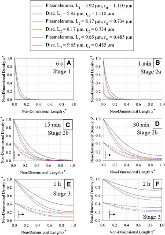
Density distribution (nondimensional) after (A) 6 s, (B) 1 min, (C) 15 min, (D) 30 min, (E) 1 h, and (F) 2 h of system evolution for three different COS starting lengths (Table 1). Three general stages of evolution are described (see text for details). In C–F, the leading edge of new disk formation is indicated by the vertical line and arrow for the shortest starting COS length (L = 5.92 μm).

Figure 6.

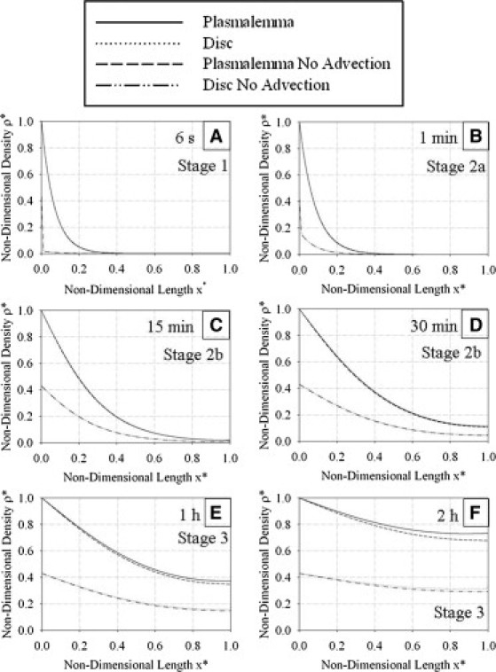
Comparison of solutions with and without advection after (A) 6 s, (B) 1 min, (C) 15 min, (D) 30 min, (E) 1 h, and (F) 2 h of system evolution. Parameters used in the solution represent the onset of the light cycle (L₁, r_t1 in Table 1). Advection does not significantly affect the solution until a time of ∼1 h of system evolution.

There were three principal stages of the mass-transfer process that were evident from the results. These three stages were all qualitatively similar for the three different points of the light cycle considered (onset, 6 h, and 10 h), but due to varying COS geometry, the results in Fig. 5 are quantitatively different. Also, since the nondimensional variables do not contain the cone tip radius, r_t, as a parameter, the solutions are not quantitatively similar. Fig. 5 A shows that Stage 1 involves the density in the plasmalemma diffusing against the fluid flow with the density in the disk region essentially remaining unchanged (except for the local influence of the boundary condition). This is typical of the first stage of the mass-transfer process, where diffusion in the plasmalemma is the dominant mechanism of transfer. Diffusion in the plasmalemma is seen to be fastest for the parameter set that represents the onset of the light cycle (which corresponds to the shortest COS length) and slowest for the parameter set that represents 10 h into the light cycle (which corresponds to the longest COS length).

Stage 2 occurs in two distinct regimes (a and b), and centers around the density front reaching the tip of the COS and mass transfer from the plasmalemma to the disk region being driven by the mass-transfer coefficient term. Recalling the definition of dimensionless time (Eq. 12), the time for the density front to reach the tip of the COS is ∼1.17 min. During the initial part of Stage 2 (Stage 2a, before one unit of characteristic time), the density distribution in the plasmalemma changes little as radiolabeled opsins transfer from the plasmalemma into the disk. This is exemplified by Fig. 5 B, which shows that after 1 min, the plasmalemma region density has changed very little from the distribution at t = 6 s, whereas the disk-region density gradually increases. Stage 2b occurs after one unit of characteristic time when the disk region and plasmalemma region have the same approximate density distribution (shown by Fig. 5 C after 15 min of system evolution and Fig. 5 D after 30 min of system evolution). In this later regime of Stage 2, both the plasmalemma and disk-region densities increase, with their density distributions remaining qualitatively the same (but quantitatively different due to void fraction effect). Once again, we see that diffusion is more rapid at the onset of the light cycle, and slowest at 10 h into the light cycle.

Stage 3, the final stage of the mass-transfer process, is marked by a gradual approach to equilibrium. This stage is exemplified by Fig. 5, E and F. Fig. 5 E, which displays the state of the system after 1 h of evolution, shows that there is now significant nonzero density in all regions of the disk and plasmalemma. Fig. 5 F, which marks 2 h of system evolution, shows that the density distribution is approaching steady-state values, as calculated analytically. All three parameter sets have the same approximate analytical solution, and it is evident from Fig. 5 F that the parameter set that represents the onset of the light cycle will reach steady state first.

Fig. 6 shows a comparison of the numeric solutions of the full system (Eqs. 13a and 13b) and the reduced system (Eqs. 15a and 15b), where scale analysis indicated that advective effects could possibly be neglected as a first approximation. The parameter set corresponding to the onset of the light cycle (with the shortest COS length) was used for this comparison because it represents the quickest diffusion time (Fig. 5) and therefore worst-case scenario. It is evident that the solution without advection is an excellent approximation to the full system for times up to 30 min (Fig. 6, A–D), or ∼26 characteristic diffusion times. Only in the final stage of the mass-transfer process (Fig. 6, E and F) do the two solutions differ. This difference becomes more pronounced as time evolves; Fig. 6 F shows that the density difference in both the disk and plasmalemma is noticeable after 2 h. Note that Fig. 6 E represents ∼51 characteristic diffusion times, and Fig. 6 F represents ∼102 characteristic diffusion times. Therefore, advection should only be neglected in the model during the earlier stages of the mass-transfer process (up to 26 characteristic diffusion times). However, we also found that this requirement may be relaxed for later stages of the light onset process. For example, for the parameter set corresponding to 10 h after the light-onset process (with L₃ = 9.65 μm), we found that the solution without advection was indistinguishable from the full solution (data not shown).

This study has bracketed one set of experimental conditions for using autoradiographic methods to visualize any preferential initial radioactive label at the base of the COS. As shown in Fig. 5 B, the base of the disk core region is preferentially labeled at 1 min, with disk label extending farther along the COS at 15, 30, and 60 min. For example, by 15 min of system evolution, the basal 20% of the COS disk region has significant label. However, at the earliest times (6 s, 1 min, and 15 min), there is very little apically directed advective flow due to new disk formation and displacement. For these three times, the numbers of new disks formed are n = 0.018, 0.18, and 2.7, respectively. (In Fig. 5, C–F, the leading edge of new disk formation is indicated by the vertical line and arrow for the shortest starting COS length (L = 5.92 μm).) However, the disk region immediately apical to these new disks (e.g., above the arrow) is also significantly labeled, with the label necessarily derived by diffusion from the plasmalemma. Even at 1 min of system evolution, with only a fraction of one new disk formed (n = 0.18), the adjacent apical disk of full size would have a label density equal to about one-half that of the new growing disks (Fig. 5 B). Because of the full size of the adjacent disk, it would contribute more signal to an autoradiogram than the new disk fragment located just basal to it.

This investigation indicates that autoradiography of labeled opsin, even at the earliest times, cannot be an effective methodology for assessing new disk formation at the base of the COS. In fact, the method cannot distinguish a static arrangement of disks from the formation of new disks, with or without recycling (discussed in Supporting Material): the label distribution that develops by diffusion along the plasmalemma basically controls the axial labeling pattern that develops in the disk array.

Conclusion

In this article, we present a detailed derivation of a simplified mathematical model for the density distribution of radiolabeled opsin in the amphibian COS. Our model relies on only one free parameter, the mass-transfer coefficient. The descriptive equations were nondimensionalized, and scale analysis showed that advective effects could be neglected as a first approximation for early times so that a simplified system could be obtained. Various analytic solution techniques were attempted, none of which were useful. Through numeric computation, the solution behavior was found to have three distinct stages. Stage 1 was marked by diffusion in the plasmalemma and no mass transfer in the disk region. Stage 2 initially involved the plasmalemma reaching a metastable state, whereas the disk region density increased, followed by a later phase that involved both the plasmalemma and disk regions increasing in density, with their distributions being qualitatively the same. The final stage, Stage 3, involved a slow relaxation to the steady state. These three stages of solution evolution should influence the experimental design of future labeling and transport studies in COSs.

Our work has assessed the limitations of autoradiography using labeled opsin as a method for investigating new disk formation in COSs. The same considerations should apply to other opsin labeling methods, e.g., genetic approaches using green fluorescent protein opsin constructs tracked by fluorescence microscopy. Genetic constructs for labeling COS proteins with much slower diffusion coefficients or which might not undergo significant diffusion, e.g., open-margin and closed-margin components, would have a much greater chance of demonstrating new disk formation and apical disk displacements. COS components that give rise to three-dimensional crystalline domains within the COS, once identified, might also be valuable targets for labeling (8,9). Lastly, future experiments should also refine the range of values for the mass-transfer coefficient, h_m.

References

- 1.Rodieck R.W. Sinauer Associates; Sunderland, MA: 1998. The First Steps in Seeing. [Google Scholar]
- 2.Nilsson S.E.G. The ultrastructure of the receptor outer segments in the retina of the leopard frog (Rana pipiens) J. Ultrastruct. Res. 1965;12:207–231. doi: 10.1016/s0022-5320(65)80016-8. [DOI] [PubMed] [Google Scholar]
- 3.Gordon J., Hood D.C. Anatomy and physiology of the frog retina. In: Fite K.V., editor. The Amphibian Visual System. Academic Press; New York: 1976. pp. 29–42. [Google Scholar]
- 4.Steinberg R.H., Fisher S.K., Anderson D.H. Disc morphogenesis in vertebrate photoreceptors. J. Comp. Neurol. 1980;190:501–508. doi: 10.1002/cne.901900307. [DOI] [PubMed] [Google Scholar]
- 5.Corless J.M., Worniałło E., Fetter R.D. Modulation of disk margin structure during renewal of cone outer segments in the vertebrate retina. J. Comp. Neurol. 1989;287:531–544. doi: 10.1002/cne.902870410. [DOI] [PubMed] [Google Scholar]
- 6.Eckmiller M.S. Cone outer segment morphogenesis: taper change and distal invaginations. J. Cell Biol. 1987;105:2267–2277. doi: 10.1083/jcb.105.5.2267. [DOI] [PMC free article] [PubMed] [Google Scholar]
- 7.Bok D. Retinal photoreceptor-pigment epithelium interactions. Friedenwald lecture. Invest. Ophthalmol. Vis. Sci. 1985;26:1659–1694. [PubMed] [Google Scholar]
- 8.Corless J.M., Worniałło E., Fetter R.D. Three-dimensional membrane crystals in amphibian cone outer segments. 1. Light-dependent crystal formation in frog retinas. J. Struct. Biol. 1994;113:64–86. doi: 10.1006/jsbi.1994.1033. [DOI] [PubMed] [Google Scholar]
- 9.Corless J.M., Worniałło E., Schneider T.G. Three-dimensional membrane crystals in amphibian cone outer segments: 2. Crystal type associated with the saddle point regions of cone disks. Exp. Eye Res. 1995;61:335–349. doi: 10.1016/s0014-4835(05)80128-9. [DOI] [PubMed] [Google Scholar]
- 10.Bok D., Young R.W. The renewal of diffusely distributed protein in the outer segments of rods and cones. Vision Res. 1972;12:161–168. doi: 10.1016/0042-6989(72)90108-3. [DOI] [PubMed] [Google Scholar]
- 11.Young R.W. The renewal of photoreceptor cell outer segments. J. Cell Biol. 1967;33:61–72. doi: 10.1083/jcb.33.1.61. [DOI] [PMC free article] [PubMed] [Google Scholar]
- 12.Young R.W. Visual cells and the concept of renewal. Invest. Ophthalmol. Vis. Sci. 1976;15:700–725. [PubMed] [Google Scholar]
- 13.Eckmiller M.S. Shifting distribution of autoradiographic label in cone outer segments and its implications for renewal. J. Hirnforsch. 1993;34:179–191. [PubMed] [Google Scholar]
- 14.Anderson D.H., Fisher S.K., Breding D.J. A concentration of fucosylated glycoconjugates at the base of cone outer segments: quantitative electron microscope autoradiography. Exp. Eye Res. 1986;42:267–283. doi: 10.1016/0014-4835(86)90061-8. [DOI] [PubMed] [Google Scholar]
- 15.Young R.W. The daily rhythm of shedding and degradation of cone outer segment membranes in the lizard retina. J. Ultrastruct. Res. 1977;61:172–185. doi: 10.1016/s0022-5320(77)80084-1. [DOI] [PubMed] [Google Scholar]
- 16.Eckmiller M.S. Distal invaginations and the renewal of cone outer segments in anuran and monkey retinas. Cell Tissue Res. 1990;260:19–28. doi: 10.1007/BF00297486. [DOI] [PubMed] [Google Scholar]
- 17.Eckmiller M.S. Morphogenesis and renewal of cone outer segments. Prog. Retin. Eye Res. 1997;16:401–441. [Google Scholar]
- 18.Bunt A.H., Klock I.B. Comparative study of 3H-fucose incorporation into vertebrate photoreceptor outer segments. Vision Res. 1980;20:739–747. doi: 10.1016/0042-6989(80)90002-4. [DOI] [PubMed] [Google Scholar]
- 19.Calvert P.D., Schiesser W.E., Pugh E.N. Diffusion of a soluble protein, photoactivatable GFP, through a sensory cilium. J. Gen. Physiol. 2010;135:173–196. doi: 10.1085/jgp.200910322. S1–S8. [DOI] [PMC free article] [PubMed] [Google Scholar]
- 20.Corless J.M., Fetter R.D., Wall-Buford D.L. Structural features of the terminal loop region of frog retinal rod outer segment disk membranes: II. Organization of the terminal loop complex. J. Comp. Neurol. 1987;257:9–23. doi: 10.1002/cne.902570103. [DOI] [PubMed] [Google Scholar]
- 21.Fetter R.D., Corless J.M. Morphological components associated with frog cone outer segment disc margins. Invest. Ophthalmol. Vis. Sci. 1987;28:646–657. [PubMed] [Google Scholar]
- 22.Corless J.M., Fetter R.D., Costello M.J. Structural features of the terminal loop region of frog retinal rod outer segment disk membranes: I. Organization of lipid components. J. Comp. Neurol. 1987;257:1–8. doi: 10.1002/cne.902570102. [DOI] [PubMed] [Google Scholar]
- 23.Molday R.S., Hicks D., Molday L. Peripherin. A rim-specific membrane protein of rod outer segment discs. Invest. Ophthalmol. Vis. Sci. 1987;28:50–61. [PubMed] [Google Scholar]
- 24.Liebman P.A., Entine G. Lateral diffusion of visual pigment in photorecptor disk membranes. Science. 1974;185:457–459. doi: 10.1126/science.185.4149.457. [DOI] [PubMed] [Google Scholar]
- 25.Liebman P.A., Weiner H.L., Drzymala R.E. Lateral diffusion of visual pigment in rod disk membranes. Methods Enzymol. 1982;81:660–668. doi: 10.1016/s0076-6879(82)81091-4. [DOI] [PubMed] [Google Scholar]
- 26.Liebman P.A. Birefringence, dichroism and rod outer segment structure. In: Snyder A.W., Menzel R., editors. Photoreceptor Optics. Springer-Verlag; New York: 1975. [Google Scholar]
- 27.Truskey G.A., Yuan F., Katz D.F. Pearson Prentice Hall; Upper Saddle River, NJ: 2004. Transport Phenomena in Biological Systems. [Google Scholar]
- 28.Lin C.C., Segel L.A. Society for Industrial and Applied Mathematics; Philadelphia, PA: 1988. Mathematics Applied to Deterministic Problems in the Natural Sciences. [Google Scholar]
- 29.Chung T.J. Cambridge University Press; Cambridge, United Kingdom: 2002. Computational Fluid Dynamics. [Google Scholar]
Associated Data
This section collects any data citations, data availability statements, or supplementary materials included in this article.