Powerful SNP-Set Analysis for Case-Control Genome-wide Association Studies

Abstract

GWAS have emerged as popular tools for identifying genetic variants that are associated with disease risk. Standard analysis of a case-control GWAS involves assessing the association between each individual genotyped SNP and disease risk. However, this approach suffers from limited reproducibility and difficulties in detecting multi-SNP and epistatic effects. As an alternative analytical strategy, we propose grouping SNPs together into SNP sets on the basis of proximity to genomic features such as genes or haplotype blocks, then testing the joint effect of each SNP set. Testing of each SNP set proceeds via the logistic kernel-machine-based test, which is based on a statistical framework that allows for flexible modeling of epistatic and nonlinear SNP effects. This flexibility and the ability to naturally adjust for covariate effects are important features of our test that make it appealing in comparison to individual SNP tests and existing multimarker tests. Using simulated data based on the International HapMap Project, we show that SNP-set testing can have improved power over standard individual-SNP analysis under a wide range of settings. In particular, we find that our approach has higher power than individual-SNP analysis when the median correlation between the disease-susceptibility variant and the genotyped SNPs is moderate to high. When the correlation is low, both individual-SNP analysis and the SNP-set analysis tend to have low power. We apply SNP-set analysis to analyze the Cancer Genetic Markers of Susceptibility (CGEMS) breast cancer GWAS discovery-phase data.

Introduction

The identification of SNPs that are associated with risk for developing complex disease is an important goal of modern genetics studies. The hope is that such knowledge can ultimately be used both for understanding the biological mechanisms underlying these diseases and for generating individualized risk profiles that are useful in a public health context. To this end, GWAS have emerged as a popular tool for identifying common genetic variants for complex disease. A standard case-control GWAS for identifying SNPs associated with disease susceptibility involves genotyping a large number of SNPs, on the order of hundreds of thousands, in thousands of individuals with the disease (cases) and thousands of healthy controls, with the goal of identifying individual loci that are associated with the outcome. Such studies have been successfully used to identify SNPs associated with susceptability to diseases such as breast cancer^1,2 (MIM 114480), prostate cancer^3–5 (MIM 176807), and type 2 diabetes^6–8 (MIM 125853).

A typical GWAS consists a discovery phase, in which an initial set of promising susceptibility loci are identified, followed by a validation stage, in which the SNPs identified in the initial discovery phase are replicated in a separate study cohort.⁹ The standard approach for analyzing GWAS in the discovery phase involves individual-SNP analysis. This mode of analysis often involves regressing the phenotype onto each individual typed SNP and generating a parametric p value. The SNPs are then ranked on the basis of their individual p values, and a threshold is set such that all SNPs with a p value less than that threshold will be pushed forward for validation. The threshold can be based on reaching a multiple-comparison-adjusted significance level or a level based on nonanalytical means.

Although the use of individual-SNP analysis has proven useful in identifying many disease-susceptibility variants, this mode of analysis may be limited in some settings because of difficulty in reaching genome-wide significance. More specifically, in order to control the overall type I error rate, the level at which each test is conducted must be adjusted. Because of the large number of considered hypotheses, the threshold for genome-wide signficance can be very extreme and difficult to attain: for a GWAS examining the effects of 500,000 SNPs, each test is conducted at the α = 10⁻⁷ level, which is very stringent.

Additionally, individual-SNP analysis is often limited by poor reproduceability; many of the highly ranked SNPs in the discovery phase are false positives and cannot be validated. This is largely due to the restricted power for detecting SNPs with small effects that are truly associated with the outcome. In particular, individual SNPs that are genotyped on GWAS platforms often show only modest effects. One explanation for this is that the true causal SNP is rarely genotyped but there are typed SNPs that are in linkage disequilibrium (LD) with the causal SNP. In this case, when individual-SNP analysis is used, the typed SNPs in LD with the causal SNP will each show only moderate effects because each typed SNP serves as an imperfect surrogate for the causal SNP. Thus, it could be advantageous to consider the joint effect of multiple SNPs in analysis,¹⁰ because it is probable that several of these markers are in LD with the causal SNP and could capture the true effect more effectively than could individual-SNP analysis. Finally, individual-SNP analysis considers only the marginal effect of each SNP and therefore fails to accommodate epistatic effects. Epistatic interactions between SNPs can contribute to disease susceptibility such that individual SNPs may show little individual effect but their interactions may have a much larger effect. Individual-SNP analysis will not be able to detect such effects, which, more generally, are difficult to find because of the large number of potential interactions.¹¹

As an alternative strategy for analysis, we propose grouping SNPs together into SNP sets along the genome and performing genome-wide tests for individual SNP sets instead of individual SNPs. SNP-set-based analysis borrows information from different but correlated SNPs that are grouped on the basis of prior biological knowledge and hence has the possibility of providing results with improved reproducibility and increased power, especially when individual-SNP effects are moderate, as well as improved interpretability. This mode of analysis proceeds via a two-step procedure. First, SNPs are assigned to SNP sets on the basis of some meaningful biological criteria (genomic features); e.g., genes. Then, tests for the association between each genomic feature and a disease phenotype are performed with the use of a logistic kernel-machine-based multilocus test, across the genome.

SNP-set analysis can prove advantageous over the standard analysis of individual SNPs. By forming SNP sets and testing each SNP set as a unit, we are reducing the number of hypotheses being tested and thus relaxing the stringent conditions for reaching genome-wide significance. Grouping SNPs together properly, we will have improved power in settings where SNPs are individually only moderately significant. In particular, though any single SNP may serve as a poor surrogate for an untyped causal SNP, by considering multiple typed SNPs, we will be better able to capture the true effect of the untyped causal SNP. Furthermore, if there are multiple independent causal SNPs, by considering their joint effects, we will have power to detect their joint activity.

To test each SNP set within a case-control GWAS, we propose a general semiparametric kernel-based testing procedure that is tailored toward high-dimensional genetic data. Specifically, this test will combine the logistic kernel-machine testing approach of Liu et al.¹² with the kernel framework suggested by Kwee et al.¹³ As we will show, the logistic kernel machine has appealing features for SNP-set analyses. The testing framework is powerful and allows for great flexibility in the functional relationship between the SNPs in a SNP set and the outcome. Thus, the method can easily account for complex SNP interactions and nonlinear effects. Combined with the ability to seamlessly adjust for covariate effects and the fast computational efficiency of our method, this flexibility gives the logistic kernel-machine-based test significant advantages over both individual SNP tests and existing multimarker tests.

Broadly speaking, our work advances the field in three important ways. First, we develop SNP-set analysis as an alternative to standard individual-SNP analysis and discuss principled approaches for forming SNP sets based on genomic features. Second, we develop a powerful statistical modeling and testing framework for genetic effects, which has a number of practical advantages over other multimarker tests: our approach is computationally efficient and naturally accommodates covariate adjustment, nonlinear effects, and epistasis. Third, we will demonstrate through thorough numerical studies and data applications that our approach can have substantially improved power over standard individual-SNP testing and, by extension, over the many multimarker tests that individual-SNP testing tends to dominate.

The remainder of this article is organized as follows. In the next section, we describe our proposed SNP-set analysis framework, including how to form SNP sets and how to subsequently test SNP sets. Then we will present simulation results comparing our approach to individual-SNP analysis and two existing multi-SNP tests. Finally, we will apply logistic kernel-machine-based SNP-set analysis to the Cancer Genetic Markers of Susceptibility (CGEMS) breast cancer data from the discovery phase. We will conclude with a brief discussion.

Material and Methods

SNP-set-based analysis borrows information from different but correlated SNPs that are grouped on the basis of prior biological knowledge and hence provides results with improved reproducibility and increased power, especially when individual-SNP effects are moderate. This mode of analysis proceeds via a two step procedure. First, across the genome, SNPs are assigned to a SNP sets on the basis of some meaningful biological criteria such as proximity to genomic features—SNP sets of a single SNP are possible. If we wished to perform genome-wide SNP-set analysis of a GWAS conducted on the Illumina HumanHap500 array by grouping SNPs on the basis of genes, we could generate approximately 18,000 SNP sets, each of which consisted of the SNPs within a single gene. For example, the 14 genotyped SNPs within the ASAH1 (MIM 228000) gene could be assigned to a single SNP set and the four genotyped SNPs within the NAT2 (MIM 612182) gene could be assigned to another SNP set, and so on. After the groupings are made, each of the 18,000 SNP sets is tested with the use of a multilocus test, and the genome-wide significance of the SNP set, e.g., each gene, is calculated. Although a number of tests have been proposed,^14,15 we consider an extension of the logistic kernel-machine test, which was developed in the gene-expression-profiling setting, which we tailor for analysis of GWAS. In this section, we describe possible methods for grouping SNPs in a genome-wide scan into SNP sets and then we present the logistic kernel-machine test for evaluating the significance of each SNP set.

Forming SNP Sets

A key aspect of our proposed approach is the formation of meaningful SNP sets. In principle, a SNP set may be formed via any grouping of SNPs, and our testing approach is still valid in the sense that the type I error rate will always be protected. However, better groupings can be made on the basis of prior biological knowledge and, if done properly, can lead to additional gains in power. In particular, the key advantages of our approach may be found in the ability to reduce the number of multiple comparisons, to harness correlation between SNPs, to measure the joint effect of independent SNPs, and to make a direct inference on a biologically meaningful genomic feature. Some natural ways of forming SNP sets that can capitalize on these advantages include grouping SNPs on the basis of genomic features. We describe below some natural grouping structures.

A natural grouping strategy is to take all SNPs that are located in or near a gene, a fundamental unit of the genome, and group them to form a SNP set. In particular, one can take all SNPs between the start and end of transcription as well as SNPs that are upstream and downstream of the gene, in order to capture regulatory regions, as a single SNP set. In grouping on the basis of known genes, we can significantly reduce the number of multiple comparisons. The SNPs on the Illumina HumanHap 500 array correspond to approximately 17,800 genes in contrast to the original 530,000 SNPs. Because we take the entire gene region, not just exonic regions, we expect to have many typed SNPs that are correlated, and thus the logistic kernel-machine test will have good power to detect a significant SNP-set effect. We could also expect multiple SNPs within a gene to be associated with disease risk, and this grouping structure would allow us to detect this effect. Testing gene-based SNP sets also makes a direct inference on the association between the gene and the case-control status.

An extension of gene-based SNP-set analysis is to group SNPs on the basis of whether they are located within a gene pathway from the Kyoto Encyclopedia of Genes and Genomes (KEGG)¹⁶ or a Gene Ontology Consortium functional category.¹⁷ Making inference on a pathway further reduces the number of multiple comparisons and still allows inference on a biologically meaningful unit. The logistic kernel-machine test will be able to harness local LD to have power and will, additionally, be able to capture true pathway effects when several SNPs in multiple genes are related to the disease.

Although many variants associated with disease have been identified within gene regions, many lie outside of the boundaries of known genes (and hence pathways). To augment coverage of the genome, a possible strategy would be to group SNPs within evolutionarily conserved regions. Increased evolutionary conservation of a genomic region is suggestive of increased importance or functionality.¹⁸ Significance of such a SNP set would potentially indicate that there is a genomic feature present that is related to disease risk, even if the feature is not well understood.

Finally, approaches to forming SNP sets that can achieve full coverage of the genome by placing all SNPs into SNP sets include grouping SNPs via a moving window or via haplotype blocks. For example, one could divide the genome into a fixed number of adjacent regions, purely on the basis of length, and treat all SNPs within a region as a SNP set. Alternatively, one could build SNP sets based on haplotype blocks, such as through Haploview.¹⁹ Both approaches will still allow us to harness local correlation to capture the effect of untyped SNPs.

An important limitation of employing a gene- or pathway-based approach is the omission of intergenic regions. However, use of additional grouping strategies, e.g., conserved regions, can augment coverage, and using the moving window and haplotype block can provide comprehensive coverage of the entire genome. Although we wish to group SNPs that are near one another to harness correlation, this does not allow us to capture multi-SNP or epistatic effects among SNPs in separate SNP sets. Using gene-pathway-based SNP sets could ameliorate this issue, because this looks across individual continuous regions. Groupings based on strategies beyond the ones that we have considered are also possible.

As noted above, we emphasize that although well-formed SNP sets can optimize the power and interpretability of our SNP-set testing strategy, our logistic kernel-machine testing approach is statistically valid irrespective of the grouping scheme. For illustration, we will focus on SNP sets formed on the basis of proximity to each of 18,000 known genes.

Genome-wide SNP-Set Testing

Although we propose our strategy as a genome-wide approach, we will present the testing procedure by focusing on testing a single SNP set.

In this paper, we assume that a population-based case-control GWAS was conducted in which n independent subjects were genotyped. To employ our SNP-set analysis approach, we first group the SNPs into SNP sets across the genome. Then, for a given SNP set containing p SNPs, let z_i1, z_i2, …, z_ip be genotype values for the SNPs in the SNP set for the i^th subject (i = 1,…,n). The case-control status for the i^th subject is denoted by y_i (y_i = 1 for cases, and y_i = 0 for controls). We assume without loss of generality that the SNPs are coded in a trinary fashion, with z_ij = 0, 1, 2 corresponding to homozygotes for the major allele, heterozygotes, and homozygotes for the minor allele, respectively. This corresponds to the commonly employed additive model of allelic effect, but we note that alternative models, such as the dominant and recessive models, are also possible and can be tested within our framework. We further assume that for each individual, an additional set of m demographic, environmental, or other confounding variables is collected. For the i^th subject, we let x_i1, x_i2, …, x_im denote the values of the covariates that we would like to adjust for. The goal of SNP-set analysis is then to test the global null of whether any of the p SNPs are related to the outcome while adjusting for the additional covariates.

In principle, many multilocus testing approaches could be used for evaluating the significance of the SNPs in the SNP set, but to harness correlation and accommodate complex relationships between the SNPs and the outcome and epistatic effects, we propose a new approach of testing the SNP set by modeling each SNP set's effect in a flexible fashion while adjusting for additional covariate effects. At the same time, to overcome the issue of the large number of degrees of freedom, our strategy will employ a test that adaptively estimates the degrees of freedom by accounting for correlation (LD) among the SNPs. Specifically, we will choose to use the logistic kernel-machine regression modeling framework and a corresponding score test.¹²

Logistic Kernel-Machine Model

In evaluating the significance of a SNP set, we need to employ a strategy that allows us to model, and subsequently test, the effects of multiple SNPs that have been grouped in a biologically meaningful fashion. The kernel-machine framework has become very popular for modeling high-dimensional biomedical data because of its ability to allow for complex/nonlinear relationships between the dependent and independent variables^20,21 while adjusting for covariate effects. We consider a logistic kernel-machine regression model for the joint effect of the SNPs in the SNP set and the additional covariates that we would like to adjust for. Under the notation above, for the i^th individual, we have the semiparametric model given by

$$\text{logit}P\left(y_{\text{i}}=1\right)={\alpha }_0+{\alpha }_1{x}_{i1}+\dots +{\alpha }_m{x}_{im}+h\left(z_{i1},z_{i2},\dots z_{ip}\right),$$ (Equation 1)

in which α₀ is an intercept term and α₁, …, α_m are regression coefficients corresponding to the environmental and demographic covariates. The SNPs, z_i1, …, z_ip, influence y_i through the general function h(·), which is an arbitrary function that that has a form defined only by a positive, semidefinite kernel function K(·, ·).

Our primary aim is to adequately model the SNPs and evaluate their effect, so h(·) is the model component in which we have primary interest because it fully determines the relationship between genotypes of the SNPs in the SNP set and disease risk. Leaving h(·) only generally specified permits a modeling framework that accommodates complex relationships between the SNPs and risk as well as epistatic effects.

We omit the mathematical details, but when using the representer theorem,²² we note that h(z_i1, z_i2, …, z_ip) in Equation 1 is equal to $h_i=h\left({\mathbf{Z}}_i\right)={\sum }_{i^{\prime }=1}^n{\gamma }_{i^{\prime }}K\left({\mathbf{Z}}_i,{\mathbf{Z}}_{i^{\prime }}\right)$ for some γ₁, …, γ_n. This shows that h(·) is fully defined by the kernel function K(·, ·). Details on the mathematical relationships and estimation may be found in Liu et al.¹² and Cristianini et al.,²⁰ but the key is that by choosing different kernel functions, we can specify different, possibly complex, bases and corresponding models. For example, if we define K(·, ·) to be the linear kernel such that $K\left({\mathbf{Z}}_i,{\mathbf{Z}}_{i^{\prime }}\right)={\sum }_{j=1}^p{z}_{ij}{z}_{i^{\prime }j}$ then we are implicitly assuming the simple logistic model defined by

$$\text{logit}P\left(y_i=1\right)={\alpha }_0+{\alpha }_1{x}_{i1}+\dots +{\alpha }_m{x}_{im}+{\beta }_1{z}_{i1}+{\beta }_2{z}_{i2}\dots +{\beta }_p{z}_{ip},$$

in which β_j is a regression coefficient corresponding to the j^th SNP. To specify a more complicated model, we need only change our choice of K(·, ·).

From the above, it is apparent that the choice of kernel changes the underlying basis for the nonparametric function governing the relationship between case-control status and the SNPs in the SNP set. Essentially, K(·, ·) is a function that projects the genotype data from the original space to another space and then h(·) is modeled linearly in this new space, such that if one considers h on the original space, it can be highly nonlinear. More intuitively, however, K(Z_i, Z_i′) can be viewed as a function that measures the similarity between two individuals, the i^th and i′^th subject, on the basis of the genotypes of the SNPs in the SNP set. Taking this perspective, many choices for K are possible. Some specific kernel functions that we can consider include the linear, identical-by-state (IBS), and weighted IBS kernels.

The linear kernel is $K\left({\mathbf{Z}}_i,{\mathbf{Z}}_{i^{\prime }}\right)={\sum }_{j=1}^p{z}_{ij}{z}_{i^{\prime }j}$ which is the usual inner product between the covariate vectors for subject i and i′. As described earlier, this kernel assumes a set of basis functions that spans the original covariate space such that one is implying a linear relationship between the logit of the probability of being a case and the genotypes of the SNPs in the SNP set; i.e., the usual multiple-logistic-regression model.

The Gaussian kernel is $K\left({\mathbf{Z}}_i,{\mathbf{Z}}_{i^{\prime }};d\right)=\exp \left\{-{\sum }_{j=1}^p{\left(z_{ij}-z_{i^{\prime }j}\right)}^2/d\right\}$ and assumes the radial basis, which is difficult to characterize with the use of an explicit set of basis functions. The class of models generated by the Gaussian kernel can be very broad and includes the linear model as a special case. Here, d is a parameter that approximately controls curvature of the kernel function, such that larger values of d correspond to smoother h functions.

The IBS kernel is $K\left({\mathbf{Z}}_i,{\mathbf{Z}}_{i^{\prime }}\right)={\sum }_{j=1}^p\left\{2I\left(z_{ij}=z_{i^{\prime }j}\right)+I\left(|z_{ij}-z_{i^{\prime }j}|=1\right)\right\}/2p$. In genetics, a possible metric for evaluating distance between individuals on the basis of genotype information is the number of alleles with IBS sharing by a pair.¹⁵ As shown by Kwee et al.,¹³ this may also be used as a valid kernel function.

The weighted IBS kernel is $K\left({\mathbf{Z}}_i,{\mathbf{Z}}_{i^{\prime }};\mathbf{w}\right)={\sum }_{j=1}^p{w}_j\left\{2I\left(z_{ij}=z_{i^{\prime }j}\right)+I\left(|z_{ij}-z_{i^{\prime }j}|=1\right)\right\}/2p$, in which $w_j=1/\sqrt{q_j}$ and q_j is the minor allele frequency (MAF) for the j^th SNP in the SNP set. The weighted IBS kernel is an extension of the IBS kernel that up-weights for similarity in rare alleles. The idea is that similarity in rare alleles is more informative than similarity in common alleles.

The ability to model data by using the Gaussian and IBS kernels is an advantage of using the kernel-machine framework, because formulating an explicit set of basis functions can be difficult. Alternative kernel functions, such as those discussed in Wei and Schaid²³ and in Mukhopadhyay et al.,²⁴ are possible and can be designed for specific data sets. To be a valid kernel function, K(·, ·) needs to be positive and semidefinite and to satisfy the conditions of Mercer's theorem.²⁰

Logistic Kernel-Machine Test

Here, our focus is on hypothesis testing, for which we need only to estimate α under the null hypothesis that h(Z_i) = 0. Therefore, we omit the technical details on estimating the genetic effect, h(Z), from the SNP set and refer the reader to Liu et al.¹²

The above modeling framework leads naturally to a powerful test for association between the SNPs in the SNP set and the case-control status. Note that the probability that the i^th subject is a case depends on the SNPs only through the function h(Z_i). Thus, in order to test whether there is a true SNP-set effect, we can consider the null hypothesis that

$$H_0:\mathbf{h}\left(\mathbf{z}\right)=0$$ (Equation 2)

against the general alternative. To test this hypothesis, Liu et al.¹² exploit the connection between the kernel-machine framework and generalized linear mixed models (GLMM). Specifically, letting K be the n × n matrix with the (i, i′)^th element equal to K(Z_i, Z_i′), it is straightforward to see that h = K γ, in which h = [h₁, …, h_n]′. We can treat h as a subject-specific random effect, then via the GLMM connection, h follows an arbitrary distribution F with a mean of zero and a variance of τK. Note that τ indexes the effect of the SNPs in the SNP set such that

$$H_0:h\left(\mathbf{Z}\right)=0\iff H_0:\tau =0.$$

Thus, we need only to test whether the indexing parameter τ is significantly different than zero. This can proceed via the variance-component score test of Zhang and Lin²⁵ using the statistic

$$Q=\frac{\left(\mathbf{y}-{\widehat{\mathbf{p}}}_0\right)\prime \mathbf{K}\left(\mathbf{y}-{\widehat{\mathbf{p}}}_0\right)}{2}.$$ (Equation 3)

in which $\text{logit}{\widehat{p}}_{0_i}={\widehat{\alpha }}_0+{\widehat{\alpha }}_1{x}_{i1}+{\widehat{\alpha }}_2{x}_{i2}+\cdots +{\widehat{\alpha }}_m{x}_{im}$. Because this is a score test, ${\widehat{\alpha }}_0$ and ${\widehat{\alpha }}_j$ are estimated under the null model, which does not contain h, so we can use the standard estimate from the logistic-regression model without the genotypes. To compute a p value for significance, we can compare Q to a scaled χ² distribution with scale parameter κ and degrees of freedom ν. Details on calculating κ and ν are found in Appendix A.

The adaptive estimation of the degrees of freedom, ν, constitutes a key advantage of the logistic kernel-machine test. In particular, if the R² between the SNPs in the SNP set increases, then ν decreases such that if all the SNPs are perfectly correlated, $\nu \to 1$. It follows that for a given h(·), higher correlation is likely to lead to higher power, suggesting that the logistic kernel-machine test improves the power for SNP-set testing by harnessing the correlation between SNPs and adaptively estimating ν.

In general, it can be difficult to identify a priori whether it is the minor allele or the major allele that is associated with increased disease risk and, equivalently, whether the minor allele is protective or deleterious. The logistic kernel-machine test is not affected by the directionality of effect, and its power is robust to whether the minor alleles of the causal SNP are protective or deleterious (or a combination of both in settings with multiple causal variants).

The testing framework considered here has similarities to those of Schaid et al.,¹⁰ Mukhopadhyay et al.,²⁴ and Wessel and Schork,¹⁵ which we describe below in that all three approaches are based on genetic distances among subjects. However, the kernel framework allows for improved flexibility in the functional relationship.

Existing Multi-SNP Tests

Although other multi-SNP tests could be used for evaluating the significance of each SNP set, the kernel machine has advantages over each of these. Here, we briefly discuss some alternative tests that fall into several different categories.

The first class of multi-SNP test encompasses the multimarker methods that are based on individual-SNP analysis. In particular, a common approach for evaluation the significance of a set of markers is to apply individual-SNP analysis by testing the individual significance of each SNP, using the most significant p value as the p value for the set of loci, and then correcting for having done multiple tests via Monte Carlo methods²⁶ or by estimating the effective number of tests.^27–29 Alternatively, the test statistics from each of the individual tests can be combined.³⁰ However, such tests still rely strongly on individual-SNP analysis, and when the individual SNPs are not in high LD with the causal variant, they may have low power, because they do not borrow information across SNPs that are frequently correlated. Furthermore, they cannot accommodate complex genetic effects and interactions. Our simulations will verify that the logistic kernel-machine test often has improved power over this class of test.

Omnibus tests for multiple SNPs or haplotypes via multivariate regression^10,31 allow for simultaneous analysis of all SNPs, but studies have shown that such methods often offer little benefit over methods based on individual-SNP analysis,^32,33 because they are based on a large number of degrees of freedom. To reduce the degrees of freedom, a set of multimarker tests that compare pairwise genetic similarity with pairwise trait similarity were proposed by Schaid et al.,¹⁴ Wessel and Schork,¹⁵ and Mukhopadhyay et al.²⁴ All three approaches are attractive; however, as noted by Mukhopadyay et al., an important limitation of Schaid et al.'s approach is that it assumes all variants have the same direction of effect, i.e., all the minor alleles for each SNP increase risk or all minor alleles decrease risk. Although the methods of Wessel and Schork and Mukhopadhyay et al. are robust to directionality, both evaluate significance via computationally expensive permutation which may be impractical for some GWAS settings. None of the three similarity based methods allow for easy covariate adjustment. The logistic kernel-machine test also considers pairwise similarity and shares the attractive nonparametric SNP effects model, but in addition to using a computationally efficient score test and being robust to directionality, the logistic kernel-machine model naturally incorporates covariate effects, an important feature. Beyond adjusting for confounders and population structure, it is often necessary to adjust for highly significant SNPs in GWAS to distinguish between settings where a particular significant marker is the causal SNP (or a SNP in high LD with the causal SNP), versus settings where additional independent markers that are associated with disease are present. A third similarity based approach by Tzeng and Zhang³⁴ can be seen as a special case of the more general logistic kernel-machine test that focuses exclusively on haplotype similarity. The need to phase sample haplotypes from genotype data incurs additional computational expense and variability—particularly for larger SNP sets.

A final class of multimarker tests consists of methods that leverage explicit population-genetics models to pinpoint the causal locus. Many involve reconstructing the sample phylogeny to guide the analysis and infer the causal mutation.^35,36 If the population-genetics model assumed is realistic and correct, such problem-specific methods should have high power. However, it is difficult to validate the assumed models, and most procedures are computationally intensive, such that in real applications the models need to be simplified. Once again, these models usually fail to allow for covariate adjustment. Computational efficiency and ease of covariate adjustment give a practical advantage to the logistic kernel-machine regression test.

Simulations

To evaluate the performance of our SNP-set analysis approach, we study the logistic kernel-machine test in the genetics framework by considering its empirical performance under a variety of settings. For simplicity of implementation, all causal SNPs in our simulations are assumed to increase disease risk, but it is important to note that none of the methods that we consider are affected by the direction of effect.

Simulations Based on the ASAH1 Gene

We first investigate the size and power of the kernel-machine testing framework under a setting in which the SNP set is generated on the basis of the LD structure of a single gene, which will allow us to better understand under which settings our SNP-set analysis approach is most advantageous. We considered the ASAH1, NAT2, and FGFR2 (MIM 176943) genes, but for clarity, we present only the simulation configurations and the results based on the ASAH1 gene. The simulations and results from use of the NAT2 and FGFR2 genes were qualitatively similar.

ASAH1, acid ceramidase 1, is a 28.5-kb-long gene with 86 HapMap SNPs and is located at 8p21.3-p22. Expression is associated with prostate cancer,³⁷ and mutations in the gene are known to be associated with Farber disease³⁸ (MIM 228000). We based our gene-specific simulations on the LD structure of the ASAH1 gene and used HAPGEN³⁹ and the CEU sample (CEPH [Utah residents with ancestry from northern and western Europe]) of the International HapMap Project⁴⁰ to generate SNP genotype data at each of the 86 loci.⁴¹ A total of 14 out of 86 SNPs are genotyped with the use of the Illumina HumanHap500 array. These will be the “typed” SNPs that we use for our simulated analysis.

We first conducted simulations to verify that the logistic kernel-machine test properly controls the type I error rate. To investigate the empirical size of our test, we conducted simulations in which we generated n/2 cases and n/2 controls under the null logistic model in which disease risk does not depend on the genotype:

$$\log \text{it}P\left(y_i=1|{\mathbf{X}}_i\right)={\alpha }_0+\mathbf{\alpha }\prime {\mathbf{X}}_i,$$ (Equation 4)

in which X_i is a vector of covariates. We considered n = 1000, 2000 and also considered the use of the linear, IBS, and weighted IBS kernels. For each choice of n and kernel function, we generated 5000 data sets by using HAPGEN. To ensure that our simulations are realistic, although our simulations generated all 86 HapMap SNPs, we apply our testing approach only to the 14 typed SNPs. Specifically, we group the 14 SNPs as a SNP set based on the ASAH1 gene and then we apply the logistic kernel-machine test to compute a p value evaluating the effect of the SNPs in the SNP set while adjusting for covariates in X. For comparison, we also analyzed the 14 typed SNPs as we would have done under an individual-SNP analysis: we tested the significance of each of the 14 SNPs individually, while again adjusting for covariates in X, and then adjusted the individual p values via a modified Bonferroni correction in which the effective number of tests was computed via two approaches. First, we used the method of Moskvina et al.²⁹ Second, we estimated the effective number of tests as the number of principal components necessary to account for 99% of the variability.⁴² The two approaches were approximately concordant. The smallest p value, corrected for the effective number of tests, was taken as the p value for the entire SNP set. The size for individual-SNP analysis testing was again the proportion of p values less than α = 0.05.

To compute the empirical power for a SNP set, we generated data sets with n/2 cases and n/2 controls under the alternative logistic model:

$$\log \text{it}P\left(y_i=1|{\mathbf{X}}_i\right)={\alpha }_0+\mathbf{\alpha }\prime {\mathbf{X}}_i+{\beta }^c{z}_i^c,$$ (Equation 5)

in which z_i^c is the genotype for the “causal” SNP, β^c is the log genetic odds ratio (OR) for the causal SNP, and X_i are a vector of additional covariates. Note that under each simulation configuration we allow only a single causal SNP. Each of the 86 HapMap SNPs was set to be the “causal” SNP in turn. Setting β^c = 0.2, which corresponds to a genetic OR of 1.22, we again considered sample sizes n = 1000, 2000. For each choice of n, and for each of the 86 causal SNPs, we generated 2000 data sets. We again applied our testing approach to each data set by grouping the 14 typed SNPs and computing a p value for the significance of the SNP set, while adjusting for covariates in X, via the logistic kernel-machine test under a linear kernel. We emphasize that only the 14 typed SNPs were used so the causal SNP is unobserved under most configurations. For each configuration, we then computed the test power as the proportion of p values less than the α level = 0.05. This was compared with the power based on the individual-SNP analysis with the modified Bonferroni correction approach described above.

Simulations Based on Randomly Sampled Genes

We also evaluate the power of our approach under settings in which the LD structure of the simulated SNP sets varied across a wide range of possible genes. Specifically, we generated 20,000 SNP sets by using HAPGEN, in which each SNP set is based on a real gene on chromosome 10. This allows for 670 possible SNP sets. Within each SNP set, we randomly selected one HapMap SNP to be the causal SNP and again generated n/2 cases and n/2 controls based on a model given by Equation 5, with β^c again fixed at 0.2 (OR = 1.22). Again treating the SNPs on the Illumina HumanHap 500K array as the typed SNPs, we tested the significance of the SNP set by using the logistic kernel-machine test under a linear kernel. We also apply the individual-SNP analysis testing procedure described above. Thus, for both our method and the competing individual-SNP analysis test, we computed 20,000 p values for significance.

Comparisons with Alternative Multi-SNP Tests

As discussed previously, in principle, any multi-SNP test can be used to test the significance of a SNP set. However, the kernel-machine test is advantageous in that it adaptively finds the degrees of freedom of the test statistic in order to account for LD between genotyped markers, can permit complex relationships between the SNPs and the outcome, naturally allows for covariate adjustment, and is computationally efficient because no permutation is required. To provide additional empirical results, we compare the logistic kernel-machine test to the similarity-based testing approach of Mukhopadhyay et al.²⁴ and the approach of Wessel and Schork,¹⁵ which has been found to perform well relative to other multi-SNP tests.²³ We assessed the power under five models and the test size under two additional models. For each of the five models examining power, 500 simulations were conducted, and 1000 simulations were conducted under the two models examining the test size. For all seven models, we assumed sample sizes of 500 cases and 500 controls, 1000 permutations were used to compute the p values for the methods of Wessel and Schork and Mukhopadhyay et al., and power and size were computed as the proportion of p values less than 0.05.

We first compare the power of the methods under four alternative models using SNP sets based on the ASAH1 gene. Under model 1, the data sets were simulated under the alternative logistic model based on Equation 5, in which the causal variant was fixed to be rs3810 (the third in the SNP set), one of the 14 typed SNPs, with β^c again fixed at 0.2 (OR = 1.22). Model 2 was similar to model 1, except that we change the causal SNP to be rs7825389 (the 69^th SNP), an untyped SNP. Model 3 was again similar to the earlier models, except that we allow for two causal variants, rs10105871 and rs7825389, which are the 63^rd and 69^th SNPs in the ASAH1 SNP set, respectively. Both SNPs are in the same LD block, and rs10105871 is typed whereas rs7825389 is untyped. The effect size for both causal SNPs was set at 0.2. Model 4 is identical to model 3, but here we have two untyped causal SNPs that are in different LD blocks, rs4377998 and rs7825389, which are the 43^rd and 69^th SNPs, respectively.

Under model 5, we compared the power under the setting considered by Mukhopadhyay et al., in which ten independent markers in Hardy-Weinberg equilibirium with MAF = 0.05 are simulated. Two of the ten markers were causal, with relative risks of 1.25 under an additive model, and all ten markers were considered to be genotyped. No additional covariates are present.

We compare the type I error rate control of the logistic kernel-machine test and the approaches by Wessel and Schork and Mukhopadhyay et al. Specifically, under model 6, we simulated null data sets based on Equation 2 and the ASAH1 gene. We applied both approaches to each of the data sets to estimate p values for the significance of the SNPs in the SNP set, and the size for each approach was estimated as the proportion of p values less than the 0.05 significance level. Model 7 is similar to model 6, but we generate an additional demographic covariate that is correlated with rs3810 (ρ = 0.065), the third SNP in the SNP set.

CGEMS Breast Cancer Data

To demonstrate the applicability and power of our approach on real data, we apply SNP-set analysis to real GWAS data and contrast our results with those found under individual-SNP analysis.

The Cancer Genetic Markers of Susceptibility (CGEMS) breast cancer study¹ was conducted to identify individual SNPs associated with breast cancer risk. To this end, in the discovery phase, 1145 cases with invasive breast cancer and 1142 controls were genotyped at 528,173 loci with the use of an Illumina HumanHap500 array. All subjects were postmenopausal women of European ancestry recruited from the Nurses Health Study. The results of the top SNPs from the discovery phase are given in Table 1. In the initial validation study, the top six SNPs as well as two others in the FGFR2 gene were genotyped in an independent set of 1776 cases and 2072 controls. A SNP within FGFR2 was validated and found to be associated with risk of breast cancer. Note that the SNPs in FGFR2 were not the top-ranked variants and that the variants within FGFR2 do not reach genome-wide significance with the use of either the Bonferroni correction or a false discovery rate (FDR) correction in the initial scan.

Table 1.

Top Results from the Discovery Phase of the CGEMS Breast Cancer GWAS

SNP	Chromosome	Gene	p Value
rs10510126	10		2.0 × 10−6
rs12505080	4		8.0 × 10−6
rs17157903	7	RELN	9.0 × 10−6
rs1219648	10	FGFR2	1.2 × 10−5
rs7696175	4	TLR1, TLR6	1.4 × 10−5
rs2420946	10	FGFR2	1.5 × 10−5
rs2107349	7	AZGP1, AZGP1P2	1.7 × 10−5
rs6497337	16	SYT17	2.0 × 10−5
rs1250255	2	FN1	3.4 × 10−5
rs10804287	2		3.8 × 10−5

To evaluate the performance of SNP-set analysis with the logistic kernel-machine-based test, we applied it to reanalysis of the CGEMS breast cancer data. Specifically, we formed SNP sets by grouping SNPs that lie within the same gene. To ensure that SNPs with possible gene-regulatory roles were also included in the SNP sets, we grouped all SNPs from 20 kb upstream of a gene to 20 kb downstream of a gene. Using these criteria, we were able to assemble a total of 17,774 SNP sets that consisted of 310,219 unique typed SNPs. We tested each of the gene-based SNP sets by using the logistic kernel-machine test under the linear kernel, the IBS kernel, and the weighted IBS kernel. SNPs were coded in the additive mode, and we adjusted for parametric effects of age group, whether the individual had hormone therapy, and the first four principal components of genetic variation to control for population stratification.⁴³

Results

Empirical Size and Power Based on the ASAH1 Gene

The size results for the logistic kernel-machine test and individual-SNP analysis are presented in Table 2. On the basis of our simulations, the logistic kernel-machine test has correct size for the kernels and has sample sizes corrected, and therefore, our overall strategy of logistic kernel-machine-based SNP-set analysis protects the type I error rate. Individual-SNP analysis with modified Bonferroni correction also has correct size. As expected, the average effective number of tests over the 5000 replicates was stable irrespective of sample size: 8.22 for n = 1000 and 8.23 for n = 2000.

Table 2.

Empirical Type I Error Rates at α = 0.05 for the Logistic Kernel-Machine Test and Individual-SNP Analysis when Applied to SNP Sets Simulated from the ASAH1 Gene

		Logististic Kernel-Machine Test
n	Individual-SNP Analysis	Linear Kernel	IBS Kernel	Weighted IBS Kernel
1000	0.049	0.052	0.046	0.055
2000	0.048	0.047	0.053	0.052

We present the empirical power results for simulation based on the ASAH1 gene in the top panel of Figure 1. The power for each testing approach and sample size is shown for each of the 86 HapMap SNPs acting as the causal SNP. On the basis of Figure 1, we can see that both methods have power when the causal SNP is in moderate or high LD with the 14 typed SNPs. In these settings, the power for our logistic kernel-machine SNP-set analysis approach tends to dominate individual-SNP analysis for both considered sample sizes, suggesting that our testing approach is an attractive alternative or auxiliary method to individual-SNP analysis. For settings in which the causal SNP was not in LD with the typed SNPs, the power was approximately at the type I error rate, as we would expect.

Figure 1.

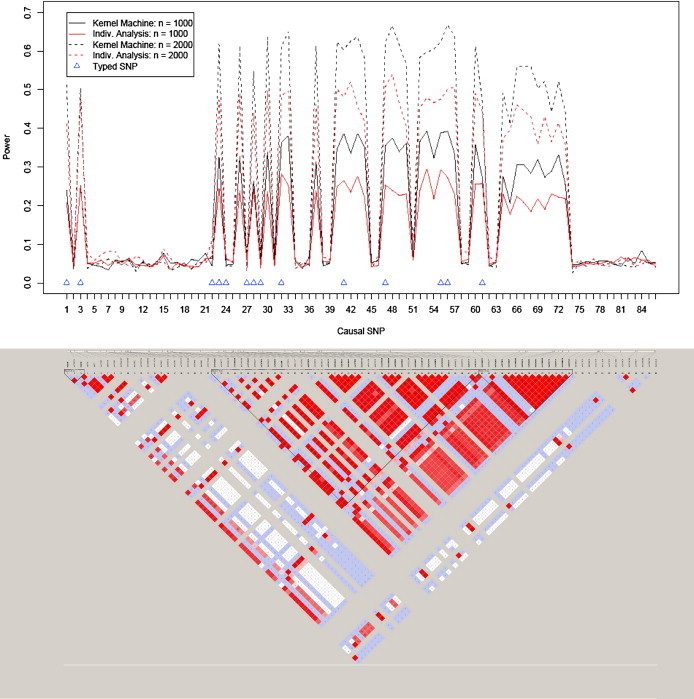
Empirical Power for SNP Sets Based on ASAH1 and LD Plot for the 86 SNPs in the ASAH1 Gene Based on the CEU Sample from the International HapMap Project

The typed SNPs are denoted with a triangle, and the bottom panel shows the LD structure of the SNPs in the ASAH1 gene.

For the purpose of clarifying the optimal conditions for our testing approach, Figure 2 shows the power for each testing approach, and sample size is again presented, but here the causal SNPs on the horizontal axis are ordered by the median R² of the causal SNP with the 14 typed SNPs. The median R² between the causal SNP and the 14 typed SNPs is plotted in the bottom panel. It is evident from the plots that the power for both testing approaches grows as a function of the median R² between the causal SNP and the typed SNPs. On the right side of the plot where the median R² is moderate to high, the kernel-machine-based testing tends to have dramatically improved power over individual-SNP analysis even when the causal SNP is genotyped. When the median R² is low, neither approach has much power. We emphasize that we consider the median R² and not the maximum R² and note that the power for the kernel-machine test is not necessarily the highest for situations in which the causal SNP is typed.

Figure 2.

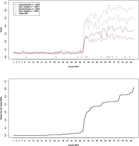
Empirical Power for SNP Sets Based on ASAH1

The SNPs on the x axis are sorted by median R² with the 14 typed SNPs, which are shown in the bottom plot.

We repeated the size and power calculations based on the ASAH1 gene for SNPs coded in a dominant model (results not shown). We also repeated power calculations for SNP sets with LD structure based on the FGFR2 and NAT2 genes. The size was again correct, and power plots are qualitatively similar.

The empirical studies show that logistic kernel-machine-based SNP-set analysis protects the type I error rate. Furthermore, except for the causal SNPs in low LD with the genotyped SNPs (for which neither method has any power beyond the type I error rate and hence any differences in power are random), the kernel-machine-based SNP-set analysis has greater power than individual-SNP analysis.

Empirical Power Based on Randomly Sampled Genes

To summarize our results, we divide the 20,000 simulations into three groups on the basis of p, the number of typed SNPs within the SNP set. Essentially, we computed power after binning the 20,000 simulations on the basis of the SNP-set size and then the median R² between the causal SNP and the typed SNPs. More specifically, we split the simulations into groups in which p ≤ 10, in which 10 < p ≤ 20, and in which 20 < p. Then we further divided each of the three groups into subgroups by sorting the simulated SNP sets on the basis of the median R² between the causal SNP and the typed SNPs and then splitting the group into 50 evenly sized subgroups. Within each subgroup, we estimated the power as the proportion of p values less than α = 0.05. For each of the groups, we plot the kernel-density smoothed power against the median R² for the subgroups in Figure 3. We need to divide the SNP sets on the basis of the number of SNPs because distantly located SNPs are uncorrelated, such that the median R² decreases with increased numbers of typed SNPs.

Figure 3.

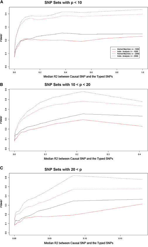
Smoothed Empirical Power Curves as a Function of Median R² between the Causal SNP and the Typed SNP for SNP Sets Based on a Range of Genes

The plots verify the earlier result that we found: the power increases as a function of the median R² between the causal SNP and the typed SNPs. If the causal SNP is uncorrelated with most typed SNPs, then we have little power to detect the SNP-set effect, but if there is any power, then the kernel-machine-based SNP-set analysis method again tends to have higher power than individual-SNP analysis. Both the overall power and the relative power of our approach to individual-SNP analysis increases as the number of typed SNPs increases. This again indicates that our approach may be a better alternative to individual-SNP analysis.

Multi-SNP Test Comparison Results

The results comparing the power and type I error rates of the logistic kernel-machine test and the Wessel and Schork approach are presented in Figure 4. As expected, if the number of independent causal SNPs is increased, the power for both approaches increases. Across the first four models, which compare the empirical power under practical settings based on the ASAH1 gene, the logistic kernel-machine test tends to have higher power than both the Wessel and Schork method, with a gain of approximately 12%–18%, and the approach of Mukhopadhyay et al., which improves little over the type I error rate. Under model 5, which assumes common MAF and no LD among typed SNPs within a gene and two causal SNPs that are genotyped, the logistic kernel-machine test and Mukhopadhyay et al.'s approach perform similarly, and both have considerably higher power than the Wessel and Schork method. Overall, these results suggest that the logistic kernel-machine test has optimal power relative to other multi-SNP tests across different patterns of LD. More interesting are the simulations comparing the type I error rate. When the demographic and environmental covariates were simulated independently of the genotype information, the size for all three tests is correct. However, when we set correlation between the covariates, which is associated with the outcome and the genotypes as being modest (0.065), failing to account for the covariates when using the Wessel and Schork and Mukhopadhyay et al. methods might possibly lead to an apparently inflated type I error rate of 25% and 10%, respectively. This illustrates the importance of evaluating the significance of SNP sets in the presence of possible confounders.

Figure 4.

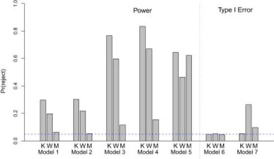
Comparison of the Power and Type I Error of the Logistic Kernel-Machine Test, the Wessel and Schork Method, and Mukhopadhyay et al.'s Approach

Abbreviations are as follows: K, logistic kernel-machine test; W, Wessel and Schork method; M, Mukhopadhyay et al.'s approach. Power and size estimates are based on 500 and 1000 simulations, respectively. The blue line shows the expected type I error rate.

Additional power simulations based on the ASAH1 gene, in which as many as four causal SNPs were used, did not yield qualitatively different results, in that the logistic kernel-machine test tended to have higher power. Because this is unlikely to be a realistic situation, given the rarity of risk-associated common variants and the relatively small regions, these results are omitted.

We note that Mukhopadhyay et al.'s approach has power similar to that of the logistic kernel-machine test under model 5. This is a setting that favors their approach. In particular, the method of Mukhopadhyay et al. is based on an ANOVA model that assumes that the effects of the modeled SNPs are constant and that the residual correlation among kernel-similarity scores is the same across all different pairs of cases or controls considered. Consequently, the method of Mukhopadhyay et al. will have excellent power when these modeling assumptions hold but may lose power when such assumptions are violated, such as under models 1–4. The logistic kernel-machine test does not make the same assumptions as the method of Mukhopadhyay et al.; for example, the effect sizes of the modeled SNPs and MAFs are allowed to vary in our approach.

Given that the power of the logistic kernel machine tends to be comparable or higher, and given the difficulties posed by failure to adjust for demographic and environmental covariates and the additional computation cost incurred by permutation, the logistic kernel-machine test appears to be an attractive approach for testing the significance of SNP sets.

CGEMS Breast Cancer Data Analysis Results

The results of our reanalysis may be found in Table 3. Using our approach and the linear kernel, we see that the SNP set formed of genetic variants close to the FGFR2 gene is now the most highly ranked SNP set, with a p value equal to 7.69 × 10⁻⁷ and an FDR q-value equal to 0.01. At that signficance level, it also reaches genome-wide significance if we apply a Bonferroni correction (α = 0.05/17, 774 = 2.8 × 10⁻⁶) or if we control the FDR. With the use of a Bonferroni correction, FGFR2 again reaches genome-wide significance if we use the IBS kernel, and if we control the FDR at 5%, it reaches significance with the weighted IBS kernel as well.

Table 3.

Top Results from the Logistic Kernel-Machine-Based SNP-Set Analysis of the CGEMS Breast Cancer Study Data

	Linear		IBS		Weighted IBS
Gene	p Value	q-Value	p Value	q-Value	p Value	q-Value
FGFR2	7.69 × 10−7	0.01	2.53 × 10−6	0.03	1.35 × 10−5	0.05
CNGA3	5.59 × 10−6	0.05	4.65 × 10−6	0.03	3.25 × 10−6	0.02
TBK1	1.30 × 10−5	0.07	3.28 × 10−6	0.03	5.48 × 10−6	0.02
VWA3B	1.53 × 10−5	0.07	7.84 × 10−6	0.03	3.99 × 10−6	0.02
PTCD3	5.50 × 10−5	0.20	9.02 × 10−6	0.03	3.78 × 10−6	0.02
XPOT	6.60 × 10−5	0.20	3.48 × 10−5	0.09	4.91 × 10−5	0.11
VAPB	9.79 × 10−5	0.22	4.51 × 10−5	0.10	8.11 × 10−5	0.14
SHC3	1.01 × 10−4	0.22	3.77 × 10−4	0.34	1.61 × 10−3	0.46
SFTPB	1.78 × 10−4	0.31	1.38 × 10−4	0.27	7.62 × 10−5	0.14
SPATA7	1.90 × 10−4	0.31	1.76 × 10−4	0.28	1.39 × 10−4	0.22

Discussion

In this article, we propose logistic kernel-machine-based SNP-set analysis as an approach for the analysis of case-control GWAS. Our approach employs prior biological knowledge to group multiple SNPs that are located near genomic features into SNP sets and then tested as a single unit. Specifically, we choose to model the SNPs in the SNP set by using a flexible, semiparametric modeling framework that is based on kernel machines, and we choose to test the effects of the SNP set via a powerful variance-components test. We illustrate our approach by using both data simulated from the International HapMap Project⁴⁰ and data from the CGEMS breast cancer GWAS of Hunter et al.,¹ and we show that our approach is an attractive alternative or auxiliary approach to individual-SNP analysis.

The logic behind our analysis strategy is that we can borrow information between different SNPs to improve the power to detect true effects. Thus, the choice of grouping can influence the power of our approach. We focused on grouping SNPs on the basis of their proximity to a known gene and noted that this allowed us to reduce multiple comparisons and to harness local LD structure in order to improve the power for capturing untyped SNPs. Using genes as the genomic features of interest allows us to map approximately 310K SNPs to 18K SNP sets. However, it may be that the causal SNP lies far from a known gene, in which case groupings based on genes (and, by extension, pathways) will fail to capture the effect of interest. To augment coverage of gene-desert regions, we can group SNPs on the basis of additional genomic features, such as evolutionarily conserved regions. Such groupings again allow us to harness local correlation. The moving-window approach will be useful for capturing all genotyped SNPs, but direct interpretation of SNP-set analysis results are more difficult, though this may not be important. Groupings via haplotype blocks are attractive because they make explicit use of the LD information. Use of haplotype blocks will allow for comprehensive coverage of the entire genome and will remove the need to explicitly predefine genomic features of interest.

Beyond harnessing local LD structure to boost power, another important feature of our approach is the ability to model the joint effect of multiple, independent, causal signals as well as possible epistatic effects. Practically, however, finding a SNP-set formation strategy that optimizes for this can be difficult. Using a gene or moving-window strategy can certainly capture multi-SNP and epistatic effects among SNPs that are located close to one another on the genome, but identification of such signals among SNPs that are distantly placed will not be possible. A potential strategy is to use existing prior biological knowledge. In particular, if multiple SNPs are expected to affect the disease risk, it is not unreasonable to expect them to lie within genes in the same pathway or in genes with similar function; hence, forming SNP sets on the basis of pathways can potentially capture such effects. Unfortunately, a systematic approach for identifying such grouping structures at the genome-wide level is not obvious. To avoid bias in our testing procedure, any grouping strategy must be made without consideration of the case-control status of the subjects in the data set. Thus, groupings must be made with the use of information from external sources, prior studies, or unsupervised statistical methods. As such, SNP-set formation strategies will improve with advances in our knowledge of the genome and genomic structures.

Although we focused our power simulations on the linear kernel, our simulation results nevertheless suggest that our approach is as powerful as individual-SNP analysis and that our approach can often have improved power over both the individual-SNP analysis strategy and other multi-SNP testing methods. In particular, we are able to show that when the causal SNP is correlated with multiple typed SNPs, our approach has higher power than individual-SNP analysis. In settings where the causal SNP is not correlated with multiple typed SNPs, simulations show that neither individual-SNP analysis nor our approach will be able to detect an effect. Recall that, here, the term individual-SNP analysis refers to correcting the smallest individual p value for the SNPs in the SNP set for multiple comparisons and using the adjusted p value as the p value for the entire SNP set. The minimum uncorrected p value for a SNP set may be smaller than the p value from the logistic kernel-machine test but would lead to a significantly inflated type I error rate. Under several settings, we found that the kernel-machine test tended to have improved power over competing multi-SNP tests while naturally allowing for covariate adjustment to protect the type I error rate when confounders are present.

We noted earlier that the linear kernel corresponds to the usual simple logistic model whereas the IBS and weighted IBS are kernels tailored specifically to genetic data and the quadratic kernel is potentially useful for modeling epistatic effects. In fact, when epistatic effects are present, the IBS kernel can allow for dramatically improved power over the linear kernel. The ability to allow for complex relationships between the SNPs by specifying just a single distance metric is an attractive feature of our approach. In practice, however, one needs to choose a kernel a priori. Although our simulations demonstrated that the size of our test is correct irrespective of the kernel used, the power will be influenced by the choice of kernel. The best way of choosing a kernel to use is unclear, because methods using the data to be tested are likely to overfit and simulations may reflect the process under which the data were simulated. Our experience in simulations and real-data applications suggests using the linear kernel for testing SNP sets in which no epistatic effects are anticipated (such SNP sets based on short regions) and using the IBS kernel otherwise. Our experience is that there is a small loss in power for use of the IBS kernel when the true effect is linear but that there is potentially a considerable loss in power when the true effect is complex and/or epistatic and the linear kernel is applied. Future research is necessary to study the power obtained when using other types of kernels.

Our numerical results lead us to recommend our kernel-machine approach for performing multi-SNP analysis across a range of realistic settings. We have shown that it has more power compared to existing popular approaches. It also has the ability to adjust for covariates. This is particularly attractive because one usually needs to control for possible population stratification and additional confounders in association studies. As noted by Mukhopadhyay et al.,²⁴ the performance of individual multi-SNP tests can depend on a range of factors, including the number of causal SNPs, effect size, and LD structure. Future research is needed for more comprehensive comparisons; e.g., in other settings and with other multi-SNP methods.

For a SNP set that is significantly associated with disease susceptibility, it is of great interest to subsequently perform fine mapping and identify the individual causal variants. One strategy that can be used is to apply a variable-selection procedure to select the “most important” SNPs. For instance, one could use a LASSO penalized logistic regression⁴⁴ to regress the case-control status on the 14 SNPs in the ASAH1 SNP set. LASSO penalized logistic regression will cause some of the regression coefficients to be estimated as exactly zero, dropping the corresponding variables from the model. Such a strategy has been used by others.^45–47 However, existing variable-selection literature does not allow for selection of features within the logistic kernel-machine regression framework in the presence of SNP-SNP interactions. The optimal strategy for quantifying the contributions of individual SNPs remains an area of considerable interest.

In addition to being able to account for complex SNP effects and to adjust for covariates, the key advantage of the logistic kernel-machine test is the ability to adaptively estimate the degrees of freedom. As discussed earlier, when the genotyped SNPs are highly correlated, the degrees of freedom of the test remain approximately constant. As a result, the strength of our method can increase as progress in genotyping technology allows for denser screens.

Appendix A

Approximating the Null Distribution of the Score Statistic for the Logistic Kernel-Machine Test

The score statistic Q defined by Equation 3 tests the null hypothesis that H₀:τ = 0 and is based on the variance-components tests developed by Zhang and Lin²⁵ and Lin⁴⁸ and adapted by Liu et al.¹² Note that this is a boundary case, so the null distribution for Q follows a complex mixture of χ². This can be approximated via the Satterthwaite method⁴⁹ as a scaled chi-square distribution, κχ²_ν, in which the scale parameter, κ, and the degrees of freedom, ν, are calculated via moment matching. Specifically, for ${\mathbf{D}}_0=\text{diag}\left({\widehat{p}}_{0_i}\left(1-{\widehat{p}}_{0_i}\right)\right)$ and P₀ = D₀ – D₀X(X′D₀X)^–1X′D₀, we define μ_Q = tr(P₀K)/2, I_ττ = tr(KP₀KP₀)/2, I_τσ = tr(P₀KP₀)/2, I_σσ = tr(P₀P′₀)/2, and ${\tilde{I}}_{\tau \tau }=I_{\tau \tau }-I_{\tau \sigma }^2/I_{\sigma \sigma }$. Then κ can be estimated as $\kappa ={\tilde{I}}_{\tau \tau }/\left(2{\mu }_Q\right)$ and we can calculate the p value for significance by comparing Q/κ to a chi-square distribution of ν degrees of freedom, χ²_ν, in which $\nu =2{\mathit{\mu }}_Q^2/{\tilde{I}}_{\tau \tau }$. The original derivation of our score test can be found in Lin,⁴⁸ in which the link function in Equation 2 of Lin is assumed to be the logit and the design matrix (Z) is set to be K^1/2. Our score statistic, Q, in Equation 4 is identical to the first term of the score statistic, U, from Equation 8 of Lin (as $\dot{\mathbf{D}}=1$ and Δ^–1W = D because the logit link is a canonical link).

Web Resources

The URLs for data presented herein are as follows:

• HAPGEN program, http://www.stats.ox.ac.uk/marchini/software/gwas/gwas.html

• Online Mendelian Inheritance in Man (OMIM), http://www.ncbi.nlm.nih.gov/Omim/

• R-functions for the logistic SNP-set kernel-machine association test, http://www.bios.unc.edu/∼mwu/software/

References

- 1.Hunter D.J., Kraft P., Jacobs K.B., Cox D.G., Yeager M., Hankinson S.E., Wacholder S., Wang Z., Welch R., Hutchinson A. A genome-wide association study identifies alleles in FGFR2 associated with risk of sporadic postmenopausal breast cancer. Nat. Genet. 2007;39:870–874. doi: 10.1038/ng2075. [DOI] [PMC free article] [PubMed] [Google Scholar]
- 2.Easton D.F., Pooley K.A., Dunning A.M., Pharoah P.D., Thompson D., Ballinger D.G., Struewing J.P., Morrison J., Field H., Luben R., SEARCH collaborators. kConFab. AOCS Management Group Genome-wide association study identifies novel breast cancer susceptibility loci. Nature. 2007;447:1087–1093. doi: 10.1038/nature05887. [DOI] [PMC free article] [PubMed] [Google Scholar]
- 3.Yeager M., Orr N., Hayes R.B., Jacobs K.B., Kraft P., Wacholder S., Minichiello M.J., Fearnhead P., Yu K., Chatterjee N. Genome-wide association study of prostate cancer identifies a second risk locus at 8q24. Nat. Genet. 2007;39:645–649. doi: 10.1038/ng2022. [DOI] [PubMed] [Google Scholar]
- 4.Gudmundsson J., Sulem P., Manolescu A., Amundadottir L.T., Gudbjartsson D., Helgason A., Rafnar T., Bergthorsson J.T., Agnarsson B.A., Baker A. Genome-wide association study identifies a second prostate cancer susceptibility variant at 8q24. Nat. Genet. 2007;39:631–637. doi: 10.1038/ng1999. [DOI] [PubMed] [Google Scholar]
- 5.Thomas G., Jacobs K.B., Yeager M., Kraft P., Wacholder S., Orr N., Yu K., Chatterjee N., Welch R., Hutchinson A. Multiple loci identified in a genome-wide association study of prostate cancer. Nat. Genet. 2008;40:310–315. doi: 10.1038/ng.91. [DOI] [PubMed] [Google Scholar]
- 6.Sladek R., Rocheleau G., Rung J., Dina C., Shen L., Serre D., Boutin P., Vincent D., Belisle A., Hadjadj S. A genome-wide association study identifies novel risk loci for type 2 diabetes. Nature. 2007;445:881–885. doi: 10.1038/nature05616. [DOI] [PubMed] [Google Scholar]
- 7.Scott L.J., Mohlke K.L., Bonnycastle L.L., Willer C.J., Li Y., Duren W.L., Erdos M.R., Stringham H.M., Chines P.S., Jackson A.U. A genome-wide association study of type 2 diabetes in Finns detects multiple susceptibility variants. Science. 2007;316:1341–1345. doi: 10.1126/science.1142382. [DOI] [PMC free article] [PubMed] [Google Scholar]
- 8.Saxena R., Voight B.F., Lyssenko V., Burtt N.P., de Bakker P.I., Chen H., Roix J.J., Kathiresan S., Hirschhorn J.N., Daly M.J., Diabetes Genetics Initiative of Broad Institute of Harvard and MIT, Lund University, and Novartis Institutes of BioMedical Research Genome-wide association analysis identifies loci for type 2 diabetes and triglyceride levels. Science. 2007;316:1331–1336. doi: 10.1126/science.1142358. [DOI] [PubMed] [Google Scholar]
- 9.Kraft P., Cox D.G. Study designs for genome-wide association studies. Adv. Genet. 2008;60:465–504. doi: 10.1016/S0065-2660(07)00417-8. [DOI] [PubMed] [Google Scholar]
- 10.Schaid D.J., Rowland C.M., Tines D.E., Jacobson R.M., Poland G.A. Score tests for association between traits and haplotypes when linkage phase is ambiguous. Am. J. Hum. Genet. 2002;70:425–434. doi: 10.1086/338688. [DOI] [PMC free article] [PubMed] [Google Scholar]
- 11.Hunter D.J., Kraft P. Drinking from the fire hose–statistical issues in genomewide association studies. N. Engl. J. Med. 2007;357:436–439. doi: 10.1056/NEJMp078120. [DOI] [PubMed] [Google Scholar]
- 12.Liu D., Ghosh D., Lin X. Estimation and testing for the effect of a genetic pathway on a disease outcome using logistic kernel machine regression via logistic mixed models. BMC Bioinformatics. 2008;9:292. doi: 10.1186/1471-2105-9-292. [DOI] [PMC free article] [PubMed] [Google Scholar]
- 13.Kwee L.C., Liu D., Lin X., Ghosh D., Epstein M.P. A powerful and flexible multilocus association test for quantitative traits. Am. J. Hum. Genet. 2008;82:386–397. doi: 10.1016/j.ajhg.2007.10.010. [DOI] [PMC free article] [PubMed] [Google Scholar]
- 14.Schaid D.J., McDonnell S.K., Hebbring S.J., Cunningham J.M., Thibodeau S.N. Nonparametric tests of association of multiple genes with human disease. Am. J. Hum. Genet. 2005;76:780–793. doi: 10.1086/429838. [DOI] [PMC free article] [PubMed] [Google Scholar]
- 15.Wessel J., Schork N.J. Generalized genomic distance-based regression methodology for multilocus association analysis. Am. J. Hum. Genet. 2006;79:792–806. doi: 10.1086/508346. [DOI] [PMC free article] [PubMed] [Google Scholar]
- 16.Kanehisa M., Goto S. KEGG: Kyoto encyclopedia of genes and genomes. Nucleic Acids Res. 2000;28:27–30. doi: 10.1093/nar/28.1.27. [DOI] [PMC free article] [PubMed] [Google Scholar]
- 17.Ashburner M., Ball C.A., Blake J.A., Botstein D., Butler H., Cherry J.M., Davis A.P., Dolinski K., Dwight S.S., Eppig J.T., The Gene Ontology Consortium Gene ontology: tool for the unification of biology. Nat. Genet. 2000;25:25–29. doi: 10.1038/75556. [DOI] [PMC free article] [PubMed] [Google Scholar]
- 18.McAuliffe J.D., Pachter L., Jordan M.I. Multiple-sequence functional annotation and the generalized hidden Markov phylogeny. Bioinformatics. 2004;20:1850–1860. doi: 10.1093/bioinformatics/bth153. [DOI] [PubMed] [Google Scholar]
- 19.Barrett J.C., Fry B., Maller J., Daly M.J. Haploview: analysis and visualization of LD and haplotype maps. Bioinformatics. 2005;21:263–265. doi: 10.1093/bioinformatics/bth457. [DOI] [PubMed] [Google Scholar]
- 20.Cristianini N., Shawe-Taylor J. Cambridge University Press; Cambridge, UK: 2000. An Introduction to Support Vector Machines and Other Kernel-Based Learning Methods. [Google Scholar]
- 21.Brown M.P., Grundy W.N., Lin D., Cristianini N., Sugnet C.W., Furey T.S., Ares M., Jr., Haussler D. Knowledge-based analysis of microarray gene expression data by using support vector machines. Proc. Natl. Acad. Sci. USA. 2000;97:262–267. doi: 10.1073/pnas.97.1.262. [DOI] [PMC free article] [PubMed] [Google Scholar]
- 22.Kimeldorf G.S., Wahba G. Some results on Tchebycheffian spline functions. J. Math. Anal. Appl. 1971;33:82–95. [Google Scholar]
- 23.Lin W.Y., Schaid D.J. Power comparisons between similarity-based multilocus association methods, logistic regression, and score tests for haplotypes. Genet. Epidemiol. 2009;33:183–197. doi: 10.1002/gepi.20364. [DOI] [PMC free article] [PubMed] [Google Scholar]
- 24.Mukhopadhyay I., Feingold E., Weeks D., Thalamuthu A. Association tests using kernel-based measures of multi-locus genotype similarity between individuals. Genet. Epidemiol. 2010;34:213–221. doi: 10.1002/gepi.20451. [DOI] [PMC free article] [PubMed] [Google Scholar]
- 25.Zhang D., Lin X. Hypothesis testing in semiparametric additive mixed models. Biostatistics. 2003;4:57–74. doi: 10.1093/biostatistics/4.1.57. [DOI] [PubMed] [Google Scholar]
- 26.Lin D.Y. An efficient Monte Carlo approach to assessing statistical significance in genomic studies. Bioinformatics. 2005;21:781–787. doi: 10.1093/bioinformatics/bti053. [DOI] [PubMed] [Google Scholar]
- 27.Cheverud J.M. A simple correction for multiple comparisons in interval mapping genome scans. Heredity. 2001;87:52–58. doi: 10.1046/j.1365-2540.2001.00901.x. [DOI] [PubMed] [Google Scholar]
- 28.Nyholt D.R. A simple correction for multiple testing for single-nucleotide polymorphisms in linkage disequilibrium with each other. Am. J. Hum. Genet. 2004;74:765–769. doi: 10.1086/383251. [DOI] [PMC free article] [PubMed] [Google Scholar]
- 29.Moskvina V., Schmidt K.M. On multiple-testing correction in genome-wide association studies. Genet. Epidemiol. 2008;32:567–573. doi: 10.1002/gepi.20331. [DOI] [PubMed] [Google Scholar]
- 30.Hoh J., Ott J. Mathematical multi-locus approaches to localizing complex human trait genes. Nat. Rev. Genet. 2003;4:701–709. doi: 10.1038/nrg1155. [DOI] [PubMed] [Google Scholar]
- 31.Zaykin D.V., Westfall P.H., Young S.S., Karnoub M.A., Wagner M.J., Ehm M.G., Inc G. Testing association of statistically inferred haplotypes with discrete and continuous traits in samples of unrelated individuals. Hum. Hered. 2002;53:79–91. doi: 10.1159/000057986. [DOI] [PubMed] [Google Scholar]
- 32.Chapman J.M., Cooper J.D., Todd J.A., Clayton D.G. Detecting disease associations due to linkage disequilibrium using haplotype tags: a class of tests and the determinants of statistical power. Hum. Hered. 2003;56:18–31. doi: 10.1159/000073729. [DOI] [PubMed] [Google Scholar]
- 33.Roeder K., Bacanu S.A., Sonpar V., Zhang X., Devlin B. Analysis of single-locus tests to detect gene/disease associations. Genet. Epidemiol. 2005;28:207–219. doi: 10.1002/gepi.20050. [DOI] [PubMed] [Google Scholar]
- 34.Tzeng J.Y., Zhang D. Haplotype-based association analysis via variance-components score test. Am. J. Hum. Genet. 2007;81:927–938. doi: 10.1086/521558. [DOI] [PMC free article] [PubMed] [Google Scholar]
- 35.Minichiello M.J., Durbin R. Mapping trait loci by use of inferred ancestral recombination graphs. Am. J. Hum. Genet. 2006;79:910–922. doi: 10.1086/508901. [DOI] [PMC free article] [PubMed] [Google Scholar]
- 36.Tachmazidou I., Verzilli C.J., De Iorio M. Genetic association mapping via evolution-based clustering of haplotypes. PLoS Genet. 2007;3:e111. doi: 10.1371/journal.pgen.0030111. [DOI] [PMC free article] [PubMed] [Google Scholar]
- 37.Saad A.F., Meacham W.D., Bai A., Anelli V., Elojeimy S., Mahdy A.E., Turner L.S., Cheng J., Bielawska A., Bielawski J. The functional effects of acid ceramidase overexpression in prostate cancer progression and resistance to chemotherapy. Cancer Biol. Ther. 2007;6:1455–1460. doi: 10.4161/cbt.6.9.4623. [DOI] [PubMed] [Google Scholar]
- 38.Li C.M., Park J.H., He X., Levy B., Chen F., Arai K., Adler D.A., Disteche C.M., Koch J., Sandhoff K., Schuchman E.H. The human acid ceramidase gene (ASAH): structure, chromosomal location, mutation analysis, and expression. Genomics. 1999;62:223–231. doi: 10.1006/geno.1999.5940. [DOI] [PubMed] [Google Scholar]
- 39.Spencer C., Su Z., Donnelly P., Marchini J. Designing genome-wide association studies: sample size, power, imputation, and the choice of genotyping chip. PLoS Genet. 2009;5:e1000477. doi: 10.1371/journal.pgen.1000477. [DOI] [PMC free article] [PubMed] [Google Scholar]
- 40.Altschuler D., Brooks L., Chakravarti A., Collins F., Daly M., Donnelly P., International HapMap Consortium A haplotype map of the human genome. Nature. 2005;437:1299–1320. doi: 10.1038/nature04226. [DOI] [PMC free article] [PubMed] [Google Scholar]
- 41.Marchini J., Howie B., Myers S., McVean G., Donnelly P. A new multipoint method for genome-wide association studies by imputation of genotypes. Nat. Genet. 2007;39:906–913. doi: 10.1038/ng2088. [DOI] [PubMed] [Google Scholar]
- 42.Gao X., Starmer J., Martin E.R. A multiple testing correction method for genetic association studies using correlated single nucleotide polymorphisms. Genet. Epidemiol. 2008;32:361–369. doi: 10.1002/gepi.20310. [DOI] [PubMed] [Google Scholar]
- 43.Price A.L., Patterson N.J., Plenge R.M., Weinblatt M.E., Shadick N.A., Reich D. Principal components analysis corrects for stratification in genome-wide association studies. Nat. Genet. 2006;38:904–909. doi: 10.1038/ng1847. [DOI] [PubMed] [Google Scholar]
- 44.Tibshirani R. Regression shrinkage and selection via the lasso. J. Roy. Statist. Soc., B. 1996;58:267–288. [Google Scholar]
- 45.Devlin B., Roeder K., Wasserman L. Analysis of multilocus models of association. Genet. Epidemiol. 2003;25:36–47. doi: 10.1002/gepi.10237. [DOI] [PubMed] [Google Scholar]
- 46.Croiseau, P., and Cordell, H. (2009). Analysis of North American Rheumatoid Arthritis Consortium data using a penalized logistic regression approach. BMC Proceedings (BioMed Central Ltd) 3, S61. [DOI] [PMC free article] [PubMed]
- 47.Szymczak S., Biernacka J.M., Cordell H.J., González-Recio O., König I.R., Zhang H., Sun Y.V. Machine learning in genome-wide association studies. Genet. Epidemiol. 2009;33(Suppl 1):S51–S57. doi: 10.1002/gepi.20473. [DOI] [PubMed] [Google Scholar]
- 48.Lin X. Variance component testing in generalised linear models with random effects. Biometrika. 1997;84:309–326. [Google Scholar]
- 49.Satterthwaite F. An approximate distribution of estimates of variance components. Biom. Bull. 1946;2:110–114. [PubMed] [Google Scholar]