The evolvability of programmable hardware

Abstract

In biological systems, individual phenotypes are typically adopted by multiple genotypes. Examples include protein structure phenotypes, where each structure can be adopted by a myriad individual amino acid sequence genotypes. These genotypes form vast connected ‘neutral networks’ in genotype space. The size of such neutral networks endows biological systems not only with robustness to genetic change, but also with the ability to evolve a vast number of novel phenotypes that occur near any one neutral network. Whether technological systems can be designed to have similar properties is poorly understood. Here we ask this question for a class of programmable electronic circuits that compute digital logic functions. The functional flexibility of such circuits is important in many applications, including applications of evolutionary principles to circuit design. The functions they compute are at the heart of all digital computation. We explore a vast space of 10⁴⁵ logic circuits (‘genotypes’) and 10¹⁹ logic functions (‘phenotypes’). We demonstrate that circuits that compute the same logic function are connected in large neutral networks that span circuit space. Their robustness or fault-tolerance varies very widely. The vicinity of each neutral network contains circuits with a broad range of novel functions. Two circuits computing different functions can usually be converted into one another via few changes in their architecture. These observations show that properties important for the evolvability of biological systems exist in a commercially important class of electronic circuitry. They also point to generic ways to generate fault-tolerant, adaptable and evolvable electronic circuitry.

1. Introduction

Biological systems are shaped by mutation and natural selection. At various levels of organization, they exhibit robustness to perturbations. That is, they are able to survive an onslaught of disruptive agents, such as hostile environments and random mutations of their genetic material. In addition, they show a remarkable ability to adapt and evolve novel properties through such random mutations [1]. In other words, biological systems are evolvable. In contrast, man-made systems are often a product of rational design, rather than biological evolution. They are often not as robust as biological systems [2], particularly to perturbations that have not been anticipated during the design stage. In other words, they are often fragile: the modification or removal of components often results in catastrophic failure. As a result, their ability to acquire novel and useful features through random change is limited. Nevertheless, there have been many attempts to design systems that exhibit high levels of robustness [3–8].

Biological systems on different levels of organization share properties important for both their robustness and their ability to evolve novel features. Biological macromolecules, such as proteins and RNA, serve to illustrate these properties. Their genotypes (amino acid or nucleotide sequences) exist in vast genotype spaces. In such a space, genotypes are neighbours if they differ in one system component (amino acids or nucleotides). A genotype's neighbourhood consists of all its neighbours. Genotypes form phenotypes, three-dimensional conformations of molecules with specific biological functions. Typically, any one phenotype can be formed by many different genotypes [9,10]. These genotypes span one or more vast genotype networks or neutral networks [9,10], connected sets of genotypes that span genotype space and that have the same phenotype. Each genotype typically has multiple neighbours with the same phenotype. Genotypes are thus typically to some extent robust to mutations changing individual system components. The existence of such genotype networks means that two molecules (genotypes G₁ and G₂) can have identical phenotypes but very different genotypes. At the same time, molecules in the neighbourhood of G₁ and G₂ can adopt very different novel phenotypes. This means that (i) small mutational changes can gradually transform G₁ into G₂, yet leave the phenotype unchanged, while (ii) mutations that occur during this transformation can uncover novel phenotypes. These properties exist in molecules such as proteins [11–13] and RNA [9,14,15], regulatory circuits [16,17] and metabolic networks [18]. We here ask whether man-made systems such as electronic circuits can display similar organizational principles, or whether there are fundamental differences between their organization and that of biological systems. The answers may help design complex yet robust man-made systems with specific functions, while facilitating their functional versatility.

Like biological systems, man-made systems are subject to two different kinds of change: (i) change in their external environment, such as changing temperature, pressure or chemical composition and (ii) change in their internal system components—the analogue of mutations. Robustness to the latter kind of change is of particular importance in biological systems, because it can facilitate innovation [1]. We will thus focus on such internal change.

Since the classic work of von Neumann [19] and McCulloch [20] on the construction of reliable systems from unreliable components, the design of man-made ‘fault-tolerant’ systems that are robust to internal change has received much attention [5–8,21,22]. Such past efforts are not limited to questions about robust system design. They also show that man-made systems such as digital circuits can be designed to adapt and evolve their function [8,23–28]. More generally, the similarities and differences between the organization of biological networks and man-made systems have been a subject of great interest [1,2,29,30].

Evolutionary principles have been applied in computer science to solve large and complex optimization and design problems, using techniques broadly classified as evolutionary computation [31,32]. These techniques implement various aspects of evolution, such as random variation, reproduction and selection in silico, to identify novel solutions to complex problems. In evolvable hardware, such techniques are applied to electronic circuits and devices. These techniques can automatically generate designs of digital circuits, as well as electronic circuits that are robust to noise and faults [8]. Hardware may be evolved intrinsically, on hardware itself, or extrinsically, using computer simulations [33]. Intrinsic evolution of hardware is often done using field-programmable gate arrays (FPGAs) [34–38].

FPGAs are silicon-based programmable digital logic circuits built from transistors. They generally consist of a two-dimensional array of ‘logic gates’, hardware units that compute elementary logic functions (e.g. OR, AND, NAND, etc.) Importantly, both the functions each gate computes, and how the gates are interconnected can be altered, hence the name ‘field-programmable’. This ability to dynamically reconfigure a circuit means that a single FPGA can serve very different computational purposes. The inputs to the entire array are binary variables, usually represented as zeroes and ones. The same holds for the array output. In other words, FPGAs compute Boolean logic functions (figure 1a,b). Which logic function a particular array computes depends on its internal gates and on its wiring. FPGAs often have a feed-forward architecture, where a gate's input can be connected to the output of any preceding gate in the array. FPGAs are widely used in various fields such as image processing, digital signal processing and high-performance computing applications, such as fast Fourier transforms [39].

Figure 1.

(Opposite.) Digital logic circuits and circuit space. (a) The standard symbols for logic gates along with the functions they represent. (b) An example of a digital logic circuit comprising four (2 × 2) gates, akin to a field-programmable gate array. The circuit comprises four logic gates, represented by the symbols shown in (a). Each of the gates has two inputs and one output. The entire array has n_I = 4 input ports and n_O = 4 output ports; the array maps a Boolean function having four input variables to four output variables. The connections between the various columns or ‘levels’ in the array are ‘feed-forward’; i.e. the inputs to each element in a column of the array can come only from the outputs of any of the elements from previous columns. There are four outputs from the array, which can be mapped to any of the four gate outputs. (c) The concept of neighbours in circuit space. The panel shows six circuits with 2 × 2 logic gates and two inputs and two outputs per circuit. The figure shows a circuit C₁ (thick ellipse) and some of its neighbours in circuit space, that is circuits that differ from it in one of the four possible kinds of elementary circuit change. For example, C₂ differs from C₁ in internal wiring, C₃ differs in the logic function computed by one of the four gates, C₅ differs in an input mapping to one of the gates and C₆, which differs in the output mapping. The circuit C₄ differs from C₁ in two elementary changes and is therefore not its neighbour in circuit space; however, it is a neighbour of C₃ and C₅. The differences between C₁ and the other circuits are shown by shaded grey boxes.

Several reasons make FPGAs attractive for our purpose. First, while usually implemented in hardware, they are conducive to computational modelling. Second, they can be built to allow a vast number of configurations that compute different functions. Third, the functions they compute are universally important in digital computation [28,39,40]. Fourth, the computational abilities of any one FPGA can be evaluated rapidly. This property facilitates our analysis below, which requires examination of vast numbers of such circuits.

In this contribution, we will systematically explore a vast set or ‘space’ of FPGA configurations or circuits, and the logic functions these circuits compute. This circuit space is an analogue to the genotype space of biological systems. Each circuit in this space corresponds to a single genotype. A circuit is completely specified through the identity of all its individual logic gates, as well as through their interconnections. The function that any one circuit computes is an analogue to a biological phenotype. Since every circuit computes exactly one function, these definitions specify a mapping from circuits (genotypes) to functions (phenotypes). We will call two circuits to be neighbours if their configuration differs minimally, either through a change in the identity of a single gate, or through an elementary change in their wiring (figure 1c). We can thus think of the circuit space as a graph, where adjacent nodes correspond to neighbouring circuits. With these concepts in mind, we will ask questions such as the following. How ‘robust’ is a typical circuit to changes in the wiring/configuration? Do neutral networks exist in this configuration space? Can circuits with significantly different configuration compute the same function? Does the organization of circuit space facilitate or hinder the adoption of novel phenotypes (logic function computations) through small numbers of gate changes?

2. Results

2.1. Circuit spaces and logic functions

The circuits we discuss in detail have n_I = 4 input and n_O = 4 output bits, as well as m columns of logic gates, each of which contain n gates. That is, a circuit consists of m × n total gates. We allow the five most commonly different kinds of two-input logic gates, that is OR, AND, XOR, NAND, NOR (figure 1a). Even for small numbers of input bits, output bits and internal gates, these specifications allow a very large number of circuits. Column 2 of the electronic supplementary material table S1 shows the size of the circuit space (number of possible circuits; see electronic supplementary material) for different circuit sizes. Even the smallest size circuit we consider (3 × 3 = 9 gates) has an astronomical number of more than 10²⁴ circuit configurations, a number that rises to more than 10¹¹⁶, for circuits with 6 × 6 gates. To represent the circuits, we use a representation based on the Cartesian genetic programming approach, developed by [41,42]; see §4.1).

As mentioned earlier, a circuit space can be viewed as a graph. Two circuits (nodes) are neighbours or connected by an edge, if they vary only by an elementary change in configuration (figure 1c). Such elementary changes affect the identity of a single logic gate (circuit C₃ in figure 1c), a change in one of the inputs to a gate (C₂), or a (single) change in the array input mappings (C₅) or output mappings (C₆). We define the shortest distance between two different circuits as the number of edges (elementary changes) in the shortest path separating them. Circuit configurations can be represented as vectors of integers that describe the inputs to each of the logic gates, the logic function computed by each gate, as well as the circuit output (see the electronic supplementary material). For a circuit of size m × n with n_O outputs, the size of this representation is 3mn + n_O, which is also the maximal distance (diameter) of the circuit space. For example, the maximal circuit distance of 4 × 4 circuits with four outputs is given by 52 elementary changes.

Below, we highlight our observations for circuits of size 4 × 4, since this number strikes a balance between circuit complexity and computational tractability. However, we will also explore how our observations depend on circuit size, by examining a broader class of circuits whose sizes range from 3 × 3 to 6 × 6 gates. We note that the complexity of the systems we study, both in terms of circuit numbers and functions, is comparable to that of genotypes and phenotypes in complex biological systems [9,11,15].

2.2. Some logic functions are frequent, others rare in circuit space

In analogy to biological systems, we define a logic function's circuit set or neutral set as the set of circuits that compute this function. Any one circuit set can consist of one or more connected neutral networks, which we define as connected subsets computing the same function. Since the circuit space for our focal circuits is very large (approx. 10⁴⁵), an exhaustive analysis is impossible. We thus sample circuits from this space at random and uniformly, that is, with equal probability. To assess the size distribution of circuit sets for different logic functions, we sampled a large number of 2 × 10⁷ circuits from the genotype space at random (see the electronic supplementary material) and recorded the function each circuit computed. Figure 2a shows a rank histogram for the logic functions a 4 × 4 circuit computes. For this plot, we assigned each function a rank based on the number of circuits in our sample that compute it. The most frequent function is assigned rank 1. The vertical axis of the figure indicates the frequency of the function, defined as the number of times the function arose divided by the sample size (2 × 10⁷). We see that a small number of functions are computed by many circuits, whereas many functions are computed by only few circuits in the sample. Electronic supplementary material, figure S1 shows analogous histograms for circuits of other sizes.

Figure 2.

(a) Frequency of various logic functions across all sampled 4 × 4 circuits. Note that both axes have a logarithmic scale; the ‘tail’ in the panel indicates that the vast majority of functions have a very low frequency; they appear only once in the circuits sampled. The distribution resembles a Zipf distribution [70]. Similar distributions have been observed earlier for RNA [9]. (b) Very different circuits can compute the same function. Shown are the distributions of the maximum distance from a starting circuit (as a fraction of circuit space diameter), at the end of a random walk of 2000 steps. (c) Functions with larger circuit sets can be computed by more distant circuits. The vertical axis indicates the maximum distance from the starting circuit at the end of a random walk of 2000 steps (as a fraction of circuit space diameter). The horizontal axis indicates the frequency of the logic function. The sizes of the circles are proportional to the number of data points with a given distance D and frequency.

For the majority of the following analyses, we consider a set of 1000 logic functions, and a representative circuit computing each function. These 1000 functions include 750 of the functions with the highest frequency, and 250 functions selected at random. The latter comprise mostly functions that occurred only once in our sample, because such functions dominate our sample. An analysis of circuits computing these functions helps understand generic properties of circuit space. To compare these generic properties with properties of individual functions, we analyse circuits computing two specific functions, the right-shift and the circular left-shift function (see the electronic supplementary material) below. We chose these two functions, because they are broadly important in a wide range of applications [43], such as image processing [44] and cryptography [45]. We note that neither function appeared in our samples of 2 × 10⁷ circuits of any size. We generated 100 distinct random circuits computing the right-shift and circular left-shift functions as described in the electronic supplementary material, and analysed properties of these sets of circuits below.

2.3. Circuits computing the same function form large connected networks

The different circuits computing a particular function might comprise a fragmented collection of circuits, where it is impossible to reach one circuit from another through small function-preserving changes. Conversely, all the circuits might lie on a single neutral network. In this case, it would be possible to navigate between circuits through small function-preserving changes. Since the entire circuit set for each function may be very large, we cannot exhaustively identify all its circuits and their connectivity in circuit space. However, we can analyse whether it is possible to reach one circuit from other circuits in the same circuit set through a number of elementary changes that leave the computed function unchanged. To examine the connectedness of circuit sets, we attempted to connect two circuits in a neutral set by means of a function-preserving random walk, as described in the electronic supplementary material. We did so for the circuit sets of the 1000 functions mentioned above. More precisely, in this analysis we focused on those functions for which our sample of 2 × 10⁷ circuits had contained more than one circuit per function. We found for each such function that all of the circuits computing the function lie on the same neutral network. In a similar fashion, we also examined the connectedness of the neutral sets of the right-shift and circular left-shift functions. Again, we found that the sets of 100 circuits that compute the right- and circular left-shift functions each belonged to the same neutral network, for 3 × 3, 4 × 4 and 5 × 5 circuits. For larger circuits (6 × 6), the amount of computation to ascertain circuit connectedness became intractable.

Overall, these analyses indicate that a large number of circuits computing the same function are accessible from one another through a series of function-preserving changes to a circuit. Even for the relatively ‘rare’ right-shift and circular left-shift functions, circuit sets are highly connected.

2.4. Very different circuits can compute the same function

The above analysis shows that neutral networks exist and connect most circuits computing a given function. We now ask how far neutral networks extend through circuit space. As mentioned above, the distance between two circuits in circuit space corresponds to the number of elementary changes required to transform one circuit to another. Within a neutral network, the maximal distance between two circuits measures how different two circuits that compute the same function can be in their organization. To estimate this maximum distance, we performed a random walk that started from a particular circuit, and subjected it to a series of small circuit changes (figure 1c) that were required to preserve the computed function. Figure 2b shows the distribution of the distance D from the starting 4 × 4 circuit, at the end of 2000 steps of a function-preserving random walk for 1000 circuits discussed above, which compute 1000 different functions. Almost 80 per cent of these random walks reach a maximal distance of circuit space diameter (D = 1). The mean distance reached by all random walks is given by D = 0.978. This means that the neutral networks of 4 × 4 circuits typically span approximately 98 per cent of the circuit space's diameter. The inset in figure 2b shows the mean and standard deviation for the other circuit sizes we considered. In all examined cases, neutral networks span a very large fraction of circuit space. Figure 2c shows the association of the maximal circuit distance (D), computed as described above, with the frequency of the logic function, for the 1000 circuits discussed above. The figure shows that the maximal distance of circuits computing the same function is generally high, regardless of the function's frequency. This maximal distance increases modestly for functions with higher frequency. In other words, functions with larger circuit sets (horizontal axis) can be computed by circuits that show greater differences in their architecture (vertical axis). Electronic supplementary material, figure S2 reveals the same pattern for circuits of other sizes. These patterns are consistent with our observation that most circuits in a circuit set belong to the same neutral network.

A vivid example of the large diameter of neutral networks is given in the electronic supplementary material, figure S3a, which shows the distribution of circuit distance after a function-preserving random walk of 2000 steps for 3 × 3 circuits computing the circular left-shift function. For 87 of the 100 circuits, this distance was equal to the circuit space's diameter. Larger circuits show the same phenomenon, as indicated by the numbers in the inset. As an example, electronic supplementary material, figure S3b shows two 3 × 3 circuits that both compute the circular left-shift function. Careful examination shows that these two circuits are maximally different. They differ in every gate, input mapping, internal wiring and output mapping, yet belong to the same neutral network. Electronic supplementary material, figure S4 shows analogous observations for circuits computing the right-shift function.

2.5. Larger circuits are more robust to configuration changes and gate failure

Neighbouring circuits in circuit space that compute the same function are neutral neighbours. We define the robustness of a circuit as the fraction of its neighbours that are neutral neighbours. This quantity is an analogue of mutational robustness in biological systems [1,15], as well as of fault-tolerance in engineering [46,47]. Figure 3a shows that the robustness of circuits computing different functions is generally high. Typically, more than half of a circuit's neighbours are neutral neighbours. Figure 3a also illustrates that circuits computing frequent functions (with large circuit sets) tend to have higher robustness, although this association is not strong. For example, function frequency and robustness of circuits computing a function show a weak positive Spearman rank correlation of r = 0.32 (p < 10⁻³⁰⁰; n = 1000) for the 4 × 4 circuits shown in the figure. Similar observations hold for circuits of other sizes (electronic supplementary material, figure S5). We also observed that different circuits computing the same function have a broad distribution of robustness, with some circuits being much more robust than others. Figure 3b shows this distribution for circuits of different size that compute the circular left-shift function. This broad distribution of robustness exists for a wide variety of functions (also see the electronic supplementary material). Some but not all of this robustness is caused by changes in gates that do not participate in a computation, because circuits are also robust when we consider only changes in gates that do contribute to a computation (electronic supplementary material, figure S6). We also analysed the robustness of circuits towards a single gate failure and observed similar trends (see figure 3c and electronic supplementary material). To illustrate how different the robustness of two circuits can be, electronic supplementary material, figure S7 shows two examples of a 3 × 3 circuit, one with low robustness of R = 0.272, another with high robustness of R = 0.753. Electronic supplementary material, figure S8 shows that the mean robustness of circuits generally increases with circuit size, for a wide range of functions with varying circuit set sizes.

Figure 3.

(a) Robustness of circuits is typically high. Circuits computing frequent functions have higher robustness, but this association is not strong. (b) Larger circuits computing circular left-shift are more robust. Note that the distribution of robustness is quite broad. (c) Circuits computing functions with higher frequency are more robust to gate failure. The distributions of robustness to gate failure, for 4 × 4 circuits computing functions of different frequencies are shown. The 1000 4 × 4 circuits have been grouped into seven bins based on the frequency of the logic functions they compute. The errors bars indicate 1 s.d.

2.6. Many new functions are accessible in the neighbourhood of ‘evolving’ circuits

In a biological system where a phenotype has a large genotype network, genotypes can change substantially without changing this phenotype. However, the phenotypes in different neighbourhoods of a genotype network can be quite different. In biological systems, this feature facilitates the exploration of new phenotypes [15,16]. If it exists in technological systems, this feature has implications on the diversity of functions that can be executed with a given amount of configuration (circuit) change, but also for the ease with which evolvable hardware can acquire new functions.

To determine whether the circuits we study have this feature, let us first define a circuit's neighbourhood as comprising all its neighbours, circuits that differ from it by a single elementary change. We explored different neighbourhoods on a neutral network through function-preserving random walks that start with a circuit C₀. During each step (circuit) of such a random walk, we first recorded the novel functions encountered in the circuit's neighbourhood. For this analysis, we defined a function as novel if it is computed by some neighbour of a circuit C_k in step k, but was not found in the neighbourhood of any previous circuit (C_i, i < k), during the random walk. Figure 4a shows the cumulative number of novel functions that becomes accessible during the random walk. This number is large and ever-increasing. The property we observe here is a typical characteristic of neutral networks in circuit space, and not a peculiarity of the neutral network of one function. For instance, electronic supplementary material, figure S9 shows the cumulative number of novel functions encountered in a function-preserving random walk for eight different circuits computing functions with widely varying frequencies.

Figure 4.

(a) Many novel functions are encountered in a circuit's neighbourhood during a function-preserving random walk. The data are based on a 4 × 4 circuit computing a function with frequency f = 5.1 × 10⁻⁵, the highest observed frequency in our sample. The horizontal axis represents the number of steps of the random walk, while the vertical axis shows the cumulative number of novel functions encountered in the neighbourhood. The evolutionary dynamics of such a random walker is identical to that of a population of circuits Nμ < 1, where N is the population size and μ is the mutation rate, the rate at which a circuit's configuration changes per circuit and generation. Such a population is monomorphic most of the time, and would visit every circuit in a neutral network with equal probability. (b) The fraction of unique functions in a neighbourhood is very high, even at small distances from the starting circuit. The horizontal axis represents the number of steps of the random walk, while the vertical axis shows the fraction u of unique functions found in the neighbourhood of C_i, at the ith step of the random walk, relative to the starting circuit C₀. (c,d) The distribution of minimal distances between neutral networks. (c) Pairs of networks computing right-shift and circular left-shift functions. (d) Pairs of networks computing other functions. See text for details.

In a next, complementary analysis, we determined the fraction of functions that are computed in the neighbourhood of a circuit during the random walk, but that are not found in the neighbourhood of the starting circuit. Specifically, we determined the fraction u, of functions that are computed by neighbours of one circuit (C_i), but not the starting circuit, C₀, as . Here, ₀ and _i represent the sets of different functions computed by circuits in the neighbourhood of the circuits C₀ and C_i, respectively, and || denotes the number of functions in the set . Figure 4b shows a steep increase in this fraction at the beginning of the random walk. Even after as few as six changes of the starting circuit C₀, over two-thirds of the functions found in the neighbourhood are new, that is, they do not occur in the neighbourhood of C₀. Beyond the distance of one circuit space diameter of 52 changes, more than 80 per cent of functions are new. This property also holds for the neutral networks of functions with a wide range of frequencies as illustrated in the electronic supplementary material, figure S10. It is clear from these observations that a large number of different functions can be computed by the neighbours of a circuit encountered during a function-preserving random walk, even at small distances from the starting circuit.

2.7. Different neutral sets are often nearby in circuit space

We next asked how far one must travel in circuit space from one neutral set to find another neutral set whose members compute a specific function. To this end, we estimated the minimal distance between circuits computing different functions (see the electronic supplementary material). On the one hand, if this distance is typically large, then it would be rather difficult to reach a circuit computing a new function from another circuit through a small series of changes to the circuit's configuration. On the other hand, if this distance is generally small, then it would typically be possible to find a specific new function through a relatively small number of elementary changes to a given circuit.

We first estimated the minimum distance for 1000 pairs of random circuits, where one circuit computed the right-shift function, and the other computed the circular left-shift function. Figure 4c shows the distribution of the resulting distances. This distribution has a mean of D = 0.13 and is skewed towards small distances. The smallest distance in this distribution was D = 0.058, corresponding to three elementary changes. In other words, it is possible to change a circuit computing the right-shift function to one computing the circular left-shift function (and vice versa) via merely three changes. We also determined the minimal distances between circuits for 5000 function pairs with low frequency in our sample (see the electronic supplementary material). Figure 4d indicates the distribution of these minimal distances. The median of this distribution is D = 0.19, implying that most distances are smaller than one-fifth of the diameter of the circuit space. This corresponds to a vanishingly small fraction of the circuit space, much less than 10⁻¹⁶. For comparison, the median distance of randomly chosen circuits is given by D = 0.85. The minimum distances we observed are thus typically quite small, especially considering that the maximum distance between any two circuits within a neutral set is often as high as the circuit space's diameter. These observations imply that a large number of new functions are accessible by making few elementary changes to any one circuit.

3. Discussion

We studied here a computational model of digital electronic circuits with various sizes. These circuits form an enormous circuit space that contains an astronomical number of circuits with different internal architecture. Circuits in this space can compute very large numbers of logic functions. Circuits computing any one function typically form large connected neutral networks that span circuit space. In other words, one can navigate from one circuit on the network to another through a series of small function-preserving changes in circuit configuration. Some functions have larger neutral networks than others. Typical member circuits of a neutral network have many neighbours that compute the same function. They are therefore robust or fault-tolerant to small changes in their architecture. A circuit that changes its architecture randomly while preserving its function explores a neutral network through a random walk. In its neighbourhood, such a random walker encounters ever-increasing numbers of novel functions. Different neutral networks are typically close-by in circuit space. That is, a few steps away from a neutral network are typically sufficient to generate a circuit that can compute an arbitrary new function.

Analogous properties have earlier been identified in biological systems on various levels of organization, such as proteins [11–13] and RNA [9,14,15], regulatory networks [16,17] and metabolic networks [18]. These properties are important for the robustness of biological systems to genetic change, and for their ability to acquire new functions (phenotypes) through random change of system parts. Our work shows that technological systems can be designed to take advantage of such properties, an observation that has multiple implications for designing evolvable hardware, as we will discuss below.

A number of limitations of our work are worth highlighting. In applications, physical factors such as temperature and voltage also play a role: there are even many fine differences between two silicon chips, such that circuits evolved on one silicon chip are not guaranteed to work on another [34]. Second, there are differences between computer simulation of a circuit and its implementation in hardware. For example, issues such as power consumption, robustness to temperature variations and trade-offs between functional flexibility and performance play a role in choosing an electronic circuit for a given task. There are also subtle aspects of semiconductor physics that circuits evolved on hardware may exploit, but that are usually avoided by designers and not considered in software simulations [34]. Our work does not address these issues. Third, some properties of our (or any other) study system may depend on the choice of representation for a circuit's architecture. An exploration of this dependency is beyond the scope of this work. Fourth, we do not know how our observations scale to much larger circuits comprising thousands to millions of gates. Fifth, because of the astronomical numbers of circuits and functions, one needs to resort to sampling to understand circuit space. The last concern is not limiting if one is interested in generic properties of this space, as we are.

Past work suggested that neutral, that is, function-preserving change is important for the ability to evolve new functions in digital logic circuitry, software and Boolean function landscapes [27,37,41,42,48–56]. Harvey & Thompson [37] have evolved circuit configurations for a tone-recognition task on hardware (FPGAs). They have also illustrated the existence of neutral networks for the specific circuit they consider. Neutrality has also been studied in cellular signalling circuits represented as Boolean networks [57]. This work illustrates various similarities of a signalling circuit's genotype–phenotype map with corresponding maps of other systems. Our work goes beyond these contributions by systematically exploring circuit space and characterizing generic features of this space, the circuits it contains and the functions they compute. It thus allows us to demonstrate the generic fault-tolerance and evolvability of an important class of technological systems.

One such general statement regards circuit robustness. The design of robust circuits using evolutionary principles has received much attention recently [4,8,22,47]. For instance, Keymeulen and collaborators evolved electronic circuits to compute the XNOR logic function. By forcing their circuits to operate in the presence of failure of individual circuit elements, they evolved circuits that were increasingly tolerant against these faults. Similarly, Hartmann & Haddow [8] used evolutionary algorithms to identify circuits that are tolerant to faults such as random gate failures and noise. These studies focus on specific circuit functions. Our work shows that the ability to design robust and fault-tolerant circuitry is a generic property and holds for many different functions. Circuits computing the same function are typically quite robust to change, but this robustness shows a broad distribution among different circuits. This means that for any one function it is possible to identify circuits that are vastly more fault-tolerant than others, as our example of circuits differing in their robustness by nearly threefold illustrated (electronic supplementary material, figure S7). Such robustness originates in the distributed architecture of a circuit and it does not require additional components such as redundant gates [22,58]. A circuit that is much more robust or fault-tolerant than another circuit thus need not have higher complexity, as measured by its number of logic gates. A related insight emerges from the observation that circuits of the same function form neutral networks in circuit space. It means that evolutionary approaches will be generally useful to identify highly robust circuits. The reason is that sufficiently large populations of circuits that evolve on a neutral network are known to accumulate in regions of the network characterized by high robustness [59,60].

A second general insight regards a circuit's ability to compute new functions. In some evolvable hardware applications, circuits that can easily change to compute new functions are highly desirable. For example, YaMoR is a modular robot composed of mechanically homogeneous modules, each of which contains a reconfigurable circuit that allows on-board self-reconfiguration [33,61]. In general, modular robots are capable of dynamically reconfiguring their structure. They are helpful in navigating unknown environments without human intervention and perform versatile tasks, such as those required during space exploration, deep sea mining, or urban search and rescue operations, essentially to navigate extreme environments inaccessible to humans [62], where the ability to reconfigure navigation circuitry would be useful. Its reconfigurable circuits endow the robots with the ability to learn. The classes of circuits we study would be especially amenable to this task, especially when it is tackled with evolutionary principles. This is because they encounter a rich diversity of novel functions in the neighbourhood of a changing circuit, even if this circuit preserves its function while undergoing random configuration change. Circuit configurations that can access more novel functions in their vicinity may be especially useful in designing systems with adaptive behaviour. Our observation that neutral networks of different functions are located close together in circuit space is also relevant in this regard. Another potential application of such adaptive hardware could be in self-repairing circuitry [63,64], where the ability of reconfiguration can be exploited to fix faults and failures. The existence of large connected neutral networks is also likely to facilitate repairs to maintain function, despite the failure of one or more parts.

The reconfiguration of FPGAs comes with an overhead, which primarily involves the reconfiguration time and reconfiguration data storage space [65]. These two reconfiguration costs are directly related to the extent of reconfiguration required. FPGAs are amenable to partial reconfiguration, where only some of their internal architecture is changed. Such partial reconfiguration can reduce the time required for reprogramming and speed up reconfiguration [66,67]. An FPGA design like ours, with its closeness of different neutral networks, can serve to minimize the number of changes necessary to compute a new function. It thus minimizes reconfiguration costs, and also permits an uninterrupted operation of the circuit, which is not possible in the case of a complete reconfiguration.

A third general observation follows from the fact that important circuit features depend on circuit complexity, as measured by the number of gates. For example, more complex circuits tend to be more robust. Electronic supplementary material, figure S11 illustrates two circuits that compute the same function. While the smaller four-gate circuit is sufficient to compute the function, it lacks robustness. The larger 16-gate circuit is much more robust. In addition, the neutral networks of larger circuits may extend farther through genotype space. Large circuits that are evolving also tend to encounter more novel functions in their neighbourhoods. Furthermore, simpler circuits may not be able to compute some logic functions. A case in point is again the space of four-gate circuits. This space comprises 4.67 × 10⁸ circuits. These circuits can compute only 4.05 × 10⁶ different functions, a small fraction of the possible 1.8 × 10¹⁹ Boolean functions with four inputs and four outputs. There are no four-gate circuits that compute the right-shift or the circular left-shift functions. These considerations show that robustness and evolvability of programmable hardware have a price: increasing system complexity.

A fourth observation regards the role of non-functional gates, system parts that are not involved in the computation a given circuit carries out. In biological systems, analogies of such parts exist. For example, many amino acids in a protein, many regulatory interactions in a gene regulation circuit and many metabolic reactions in a metabolic reaction network may appear as ‘non-functional’ or ‘dispensable’ [16,18,68,69]. One might be tempted to call such system parts to be ‘junk’ parts. However, we now know that such parts play a crucial role for evolvability, and it is precisely their ability to vary freely in some environments that allows biological systems to evolve novel phenotypes. For example, in laboratory evolution experiments, proteins with new function evolve often through changes that do not affect the protein's principal function [68]. Unused parts in our circuits have precisely the same role, and they should thus not be named junk. These observations also agree with our analysis of circuit complexity. Circuits of a minimal size may have the merit of computing a function in an elegant and simple way. At the same time, they would be utterly unevolvable. This is why evolvability comes at the price of high complexity.

A choice of circuit size is only one of many choices one has to make in designing reconfigurable hardware. We have explored a particular class of circuits with a limited number of logic gates and feed-forward connections. Many other choices are possible. Some of them may facilitate fault-tolerance and adaptability, others may impair it. The exploration of such system classes, as well as completely different technological systems with complex architectures and diverse functionality provides a fertile ground for future research.

4. Methods

4.1. Representation of FPGAs

We employ a simple vector representation of an FPGA that involves the use of three integers per gate to identify the two inputs and the gate's logic function. To this list we append a list of outputs from the array. The length of this representation is therefore 3mn + n_O, for an FPGA of size m × n with n_O outputs, i.e. computing an n_O-bit Boolean function. This is also the diameter of the circuit space. The array inputs are numbered from 1, … , n_I, while the output of each gate is numbered sequentially, from n_I + 1, … , n_I + mn. We consider five gates, viz. OR, AND, XOR, NAND, NOR, which are the most commonly used two-input logic gates. These five gates are represented by integers from 1 to 5. The list of outputs merely indicates which of the mn gate outputs (numbered n_I + 1, … , n_I + mn) are mapped to each of the FPGA array output bits. This representation is similar to the one that is conventionally used in Cartesian genetic programming [25]. The following is a vector representation of the circuit shown in the top panel of the electronic supplementary material, figure S3b: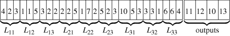

where L_ij represents a logic gate in the array in column i and row j. This vector representation also enables us to easily compute the distance between two circuits—it is the number of ‘bits’ in the representation that differ between the two circuits, or the Hamming distance between the two vectors. Neighbours of a circuit represent elementary changes to the wiring of the FPGA. Specifically, the neighbours of a circuit differ exactly in one of the bits of the vector representation (a Hamming distance of one).

4.2. Random sampling of circuits

We consider circuits of size m × n that map n_I inputs to n_O outputs. Each of the mn logic gates can compute one of the five logic functions (n_G = 5), which are listed in figure 1a. The circuits we study can be represented by a vector of length 3mn + n_O (see the electronic supplementary material). We generate a random circuit by selecting input mappings, gate configurations and output mappings at random, with uniform probability among the set of all possible choices. That is, to each digit in the representation, we assign a value based on an integer drawn from the discrete uniform distribution of all permissible values. This ensures that each circuit in the space is equally likely to appear during sampling. Specifically, we first choose an input mapping from 2n uniformly distributed random integers in [1,n_I]; mappings that do not use all the n_I inputs are not permissible. Second, we choose the logic function of each gate via a random integer in [1,n_G]. For a circuit of size m × n, we choose the mn gates function independently. Third, we choose the two inputs of each gate such that for an element in column c, the permissible inputs correspond to integers in [1,n(c − 1)], and are chosen uniformly from this set.

4.3. Fraction of neutral neighbours

We consider two circuits to be neighbours of one another if they differ by an elementary configuration change, i.e. the change in logic function computed by one of the gates of the array, or the change in an input to one of the elements of the array, or a single change in the mapping of inputs or outputs (figure 1c). The vector representation that we have described earlier facilitates the enumeration of neighbours of a particular circuit—each neighbour of a circuit differs in exactly one digit of the representation.

Every circuit has a large number of neighbours; for example, there are mn(n_G − 1) neighbours for an m × n circuit, which vary only in the configuration of one of the mn gates. This large number arises from the fact that each of the mn gates can be varied, one at a time, to any of the remaining n_G − 1 possible gate configurations. There are many additional neighbouring circuits that differ in wiring or input–output mappings. To identify the fraction of a circuit's neutral neighbours, that is, neighbours that compute the same function, we simply enumerated all neighbours and determined the function each neighbour computed. We performed this analysis for 1000 circuits, each computing one of the 1000 logic functions we considered.

To estimate a circuit's robustness to gate failure, we generated neighbours of the circuit that differ from it by the failure of a single gate. We define a failed gate as a gate that produces an output value of zero for any possible input. A circuit of size m × n has mn circuit variants with a single gate failure. We computed the fraction of these variants that computed the same function as the circuit, despite their failed gate.

Details on methods for the estimation of the connectedness of two circuits in circuit space and the computation of the minimal distance between two neutral networks are described in the electronic supplementary material.

References

- 1.Wagner A. 2005. Robustness and evolvability in living systems. Princeton, NJ: Princeton University Press [Google Scholar]
- 2.Kitano H. 2005. Scientific and technical challenges for systems biology. In Systems biology (eds Alberghina L., Westerhoff H. V.), pp. 373–385 Topics in Current Genetics, vol. 13 Berlin/Heidelberg, Germany: Springer; 10.1007/b137124 (doi:10.1007/b137124) [DOI] [Google Scholar]
- 3.Ray T. S. 1991. Is it alive or is it GA? In Proc. of the 1991 Int. Conf. on Genetic Algorithms (eds Belew R. K., Booker L. B.), pp. 527–534 CA, USA: Morgan Kaufmann [Google Scholar]
- 4.Thompson A. 1996. Evolutionary techniques for fault tolerance. In Proc. UKACC Int. Conf. on Control 1996 (CONTROL’96) (eds Higuchi T., Iwata M., Liu W.), pp. 693–698 IEE Conference Publication no. 427 [Google Scholar]
- 5.Tempesti G., Mange D., Stauffer A. 1997. A robust multiplexer-based FPGA inspired by biological systems. J. Syst. Archit. 43, 719–733 10.1016/S1383-7621(94)00312-2 (doi:10.1016/S1383-7621(94)00312-2) [DOI] [Google Scholar]
- 6.Millet P., Heudin J.-C. 1998. Fault tolerance of a large-scale mind architecture using a genetic algorithm. In Evolvable systems: from biology to hardware, pp. 356–363 Berlin/Heidelberg, Germany: Springer [Google Scholar]
- 7.Bradley D. W., Tyrrell A. M. 2000. Immunotronics: hardware fault tolerance inspired by the immune system. In ICES ‘00: Proc. of the 3rd Int. Conf. on Evolvable Systems, pp. 11–20 London, UK: Springer [Google Scholar]
- 8.Hartmann M., Haddow P. 2004. Evolution of fault-tolerant and noise-robust digital designs. IEE Proc. Comput. Digital Tech. 151, 287–294 10.1049/ip-cdt:20040014 (doi:10.1049/ip-cdt:20040014) [DOI] [Google Scholar]
- 9.Schuster P., Fontana W., Stadler P. F., Hofacker I. L. 1994. From sequences to shapes and back: a case study in RNA secondary structures. Proc. R. Soc. Lond. B 255, 279–284 10.1098/rspb.1994.0040 (doi:10.1098/rspb.1994.0040) [DOI] [PubMed] [Google Scholar]
- 10.Wagner A. 2008. Neutralism and selectionism: a network-based reconciliation. Nat. Rev. Genet. 9, 965–974 10.1038/nrg2473 (doi:10.1038/nrg2473) [DOI] [PubMed] [Google Scholar]
- 11.Lipman D. J., Wilbur W. J. 1991. Modelling neutral and selective evolution of protein folding. Proc. R. Soc. Lond. B 245, 7–11 10.1098/rspb.1991.0081 (doi:10.1098/rspb.1991.0081) [DOI] [PubMed] [Google Scholar]
- 12.Babajide A., Hofacker I. L., Sippl M. J., Stadler P. F. 1997. Neutral networks in protein space: a computational study based on knowledge-based potentials of mean force. Fold Des. 2, 261–269 [DOI] [PubMed] [Google Scholar]
- 13.Ferrada E., Wagner A. 2008. Protein robustness promotes evolutionary innovations on large evolutionary time-scales. Proc. R. Soc. B 275, 1595–1602 10.1098/rspb.2007.1617 (doi:10.1098/rspb.2007.1617) [DOI] [PMC free article] [PubMed] [Google Scholar]
- 14.Huynen M. A. 1996. Exploring phenotype space through neutral evolution. J. Mol. Evol. 43, 165–169 [DOI] [PubMed] [Google Scholar]
- 15.Wagner A. 2008. Robustness and evolvability: a paradox resolved. Proc. R. Soc. B 275, 91–100 10.1098/rspb.2007.1137 (doi:10.1098/rspb.2007.1137) [DOI] [PMC free article] [PubMed] [Google Scholar]
- 16.Ciliberti S., Martin O. C., Wagner A. 2007. Innovation and robustness in complex regulatory gene networks. Proc. Natl Acad. Sci. USA 104, 13 591–13 596 10.1073/pnas.0705396104 (doi:10.1073/pnas.0705396104) [DOI] [PMC free article] [PubMed] [Google Scholar]
- 17.Munteanu A., Solé R. V. 2008. Neutrality and robustness in evo-devo: emergence of lateral inhibition. PLoS Comput. Biol. 4, e1000 226. 10.1371/journal.pcbi.1000226 (doi:10.1371/journal.pcbi.1000226) [DOI] [PMC free article] [PubMed] [Google Scholar]
- 18.Rodrigues J. F. M., Wagner A. 2009. Evolutionary plasticity and innovations in complex metabolic reaction networks. PLoS Comput. Biol. 5, e1000 613. 10.1371/journal.pcbi.1000613 (doi:10.1371/journal.pcbi.1000613) [DOI] [PMC free article] [PubMed] [Google Scholar]
- 19.von Neumann J. 1956. Probabilistic logics and synthesis of reliable organisms from unreliable components. In Automata studies (eds Shannon C., McCarthy J.), pp. 43–98 Princeton, NJ: Princeton University Press [Google Scholar]
- 20.McCulloch W. S. 1960. The reliability of biological systems. In Self-organizing systems (eds Yovits M. C., Cameron S.), pp. 264–281 New York, NY: Pergamon Press [Google Scholar]
- 21.Coren I., Krishna C. 2007. Fault-tolerant systems. CA, USA: Morgan Kauffman [Google Scholar]
- 22.Macia J., Solé R. V. 2009. Distributed robustness in cellular networks: insights from synthetic evolved circuits. J. R. Soc. Interface 6, 393–400 10.1098/rsif.2008.0236 (doi:10.1098/rsif.2008.0236) [DOI] [PMC free article] [PubMed] [Google Scholar]
- 23.Koza J. 1992. Genetic programming. Oxford, Oxfordshire: Oxford University Press [Google Scholar]
- 24.Haddow P., Tufte G. 2000. An evolvable hardware FPGA for adaptive hardware. In Proc. of the 2000 Congress on Evolutionary Computation, La Jolla, CA, 16–19 July 2000, vol. 1, pp. 553–560 Washington, DC: IEEE 10.1109/CEC.2000.870345 (doi:10.1109/CEC.2000.870345) [DOI] [Google Scholar]
- 25.Miller J. F., Job D., Vassilev V. K. 2000. Principles in the evolutionary design of digital circuits—Part II. Genetic programming and evolvable machines 1, 259–288 10.1023/A:1010066330916 (doi:10.1023/A:1010066330916) [DOI] [Google Scholar]
- 26.Yu T., Miller J. 2001. Neutrality and the evolvability of Boolean function landscape. In Genetic programming (eds Miller J., Tomassini M., Lanzi P. L., Ryan C., Tettamanzi A. G. B., Langdon W. B.), vol. 2038 of Lecture Notes in Computer Science, chap. 16, pp. 204–217 Berlin/Heidelberg, Germany: Springer; 10.1007/3-540-45355-5_16 (doi:10.1007/3-540-45355-5_16) [DOI] [Google Scholar]
- 27.Banzhaf W., Leier A. 2006. Evolution on neutral networks in genetic programming. In Genetic programming theory and practice III, vol. 9, pp. 207–221 USA: Springer. [Google Scholar]
- 28.Greenwood G. 2007. Introduction to evolvable hardware. New York, NY: IEEE Press [Google Scholar]
- 29.Ferrer-Cancho R., Janssen C., Solé R. V. 2001. Topology of technology graphs: small world patterns in electronic circuits. Phys. Rev. E. 64, 046119. [DOI] [PubMed] [Google Scholar]
- 30.Solé R. V., Ferrer-Cancho R., Montoya J. M., Valverde S. 2002. Selection, tinkering, and emergence in complex networks. Complex 8, 20–33 10.1002/cplx.10055 (doi:10.1002/cplx.10055) [DOI] [Google Scholar]
- 31.Holland J. 1992. Adaptation in natural and artificial systems. Cambridge, UK: MIT Press [Google Scholar]
- 32.Mitchell M. 1996. An introduction to genetic algorithms. Cambridge, UK: MIT Press [Google Scholar]
- 33.Upegui A., Sanchez E. 2008. Reconfigurable computing, chap. Evolvable FPGAs, pp. 725–752 San Diego, CA: Morgan Kaufmann [Google Scholar]
- 34.Thompson A. 1995. Evolving electronic robot controllers that exploit hardware resources. In Advances in artificial life: Proc. 3rd Eur. Conf. on Artificial Life (ECAL95) (eds Morán F., Moreno A., Merelo J. J., Chacon P.), vol. 929 of LNAI, pp. 640–656 Berlin, Germany: Springer [Google Scholar]
- 35.Thompson A. 1996. Silicon evolution. In GECCO ‘96: Proc. of the 1st Annual Conf. on Genetic Programming, pp. 444–452 Cambridge, MA, USA: MIT Press [Google Scholar]
- 36.Thompson A. 1997. An evolved circuit, intrinsic in silicon, entwined with physics. In First Int. Conf. on Evolvable systems: from biology to hardware, ICES96, Tsukuba, Japan, 7–8 October 1996 (eds Higuchi T., Iwata M., Liu W.), pp. 390–405 Berlin/Heidelberg, Germany: Springer. [Google Scholar]
- 37.Harvey I., Thompson A. 1996. Through the labyrinth evolution finds a way: a silicon ridge. In ICES '96: Proc. of the 1st Int. Conf. on Evolvable Systems, Tsukuba, Japan, 7–8 October 1996 (eds Higuchi T., Iwata M., Lei W.), pp. 406–422 London, UK: Springer. [Google Scholar]
- 38.Hollingworth G., Smith S., Tyrell A. 2000. The intrinsic evolution of virtex devices through internet reconfigurable logic. In ICES '00: Proc. of the Third Int. Conf. on Evolvable Systems, Edinburgh, UK, 17–19 April 2000 (eds Miller J., Thompson A., Thompson P., Fogarty T. C.), pp. 72–79 London, UK: Springer. [Google Scholar]
- 39.Meyer-Baese U. 2007. Digital signal processing with field programmable gate arrays. Berlin, Germany: Springer [Google Scholar]
- 40.Balch M. 2003. Complete digital design. New York, NY: McGraw-Hill [Google Scholar]
- 41.Miller J. F. 1999. An empirical study of the efficiency of learning Boolean functions using a Cartesian genetic programming approach. In Proc. of the Genetic and Evolutionary Computation Conference, vol. 2 (eds Banzhaf W., Daida J., Eiben A. E., Garzon M. H., Honavar V., Jakiela M., Smith R. E.), pp. 1135–1142 FL, USA: Morgan Kaufmann [Google Scholar]
- 42.Miller J. F., Thomson P. 2000. Cartesian genetic programming. In EuroGP (eds Poli R., Banzhaf W., Langdon W. B., Miller J. F., Nordin P., Fogarty T. C.), vol. 1802 of Lecture Notes in Computer Science, pp. 121–132 Springer [Google Scholar]
- 43.Irvine K. 2007. Assembly language for Intel-based computers. Upper Saddle River, NJ: Pearson Prentice Hall [Google Scholar]
- 44.Fisher R. 1997. Hypermedia image processing reference. New York, NY: Wiley [Google Scholar]
- 45.Stallings W. 2006. Cryptography and network security. Upper Saddle River, NJ: Pearson/Prentice Hall [Google Scholar]
- 46.White R., Miles F. 1996. Principles of fault tolerance. In Proc. of the 11th Annual Applied Power Electronics Conf. and Exposition. APEC '96, San Jose, CA, 3–7 March 2006, vol. 1, pp. 18–25 Washington, DC: IEEE 10.1109/APEC.1996.500416 (doi:10.1109/APEC.1996.500416) [DOI] [Google Scholar]
- 47.Keymeulen D., Zebulum R., Jin Y., Stoica A. 2000. Fault-tolerant evolvable hardware using field-programmable transistor arrays. IEEE Trans. Reliability 49, 305–316 10.1109/24.914547 (doi:10.1109/24.914547) [DOI] [Google Scholar]
- 48.Banzhaf W. 1994. Genotype–phenotype-mapping and neutral variation–a case study in genetic programming. In PPSN III: Proc. Int. Conf. on Evolutionary Computation. The Third Conference on Parallel Problem Solving from Nature (eds Yu T., Riolo R., Worzel B.), pp. 322–332 London, UK: Springer [Google Scholar]
- 49.Ebner M. 1999. On the search space of genetic programming and its relation to nature's search space. In Proc. 1999 Congress on Evolutionary Computation, 1999. CEC '99, Washington, DC, 6–9 July 1999, vol. 2. Washington, DC: IEEE; 10.1109/CEC.1999.782609 (doi:10.1109/CEC.1999.782609) [DOI] [Google Scholar]
- 50.Ebner M., Langguth P., Albert J., Shackleton M., Shipman R. 2001. On neutral networks and evolvability. In Proc. of the 2001 Congress on Evolutionary Computation, Seoul, South Korea, 27–30 May 2001, vol. 1, pp. 1–8 Washington, DC: IEEE 10.1109/CEC.2001.934363 (doi:10.1109/CEC.2001.934363) [DOI] [Google Scholar]
- 51.Ebner M., Shackleton M., Shipman R. 2001. How neutral networks influence evolvability. Complexity 7, 19–33 10.1002/cplx.10021 (doi:10.1002/cplx.10021) [DOI] [Google Scholar]
- 52.Vassilev V. K., Miller J. F. 2000. The advantages of landscape neutrality in digital circuit evolution. In ICES '00: Proc. of the 3rd Int. Conf. on Evolvable Systems, pp. 252–263 London, UK: Springer [Google Scholar]
- 53.Yu T., Miller J. 2002. Finding needles in haystacks is not hard with neutrality. In Genetic programming (eds Foster J. A., Lutton E., Miller J., Ryan C., Tettamanzi A.), vol. 2278 of Lecture Notes in Computer Science, chap. 2, pp. 46–54 Berlin/Heidelberg, Germany: Springer; 10.1007/3-540-45984-7_2 (doi:10.1007/3-540-45984-7_2) [DOI] [Google Scholar]
- 54.Yu T., Miller J. F. 2006. Through the interaction of neutral and adaptive mutations, evolutionary search finds a way. Artif. Life 12, 525–551 10.1162/artl.2006.12.4.525 (doi:10.1162/artl.2006.12.4.525) [DOI] [PubMed] [Google Scholar]
- 55.Collins M. 2006. Finding needles in haystacks is harder with neutrality. Genetic Programm. Evol. Mach. 7, 131–144 10.1007/s10710-006-9001-y (doi:10.1007/s10710-006-9001-y) [DOI] [Google Scholar]
- 56.Miller J. F., Smith S. L. 2006. Redundancy and computational efficiency in cartesian genetic programming. IEEE Trans. Evol. Comput. 10, 167–174 10.1109/TEVC.2006.871253 (doi:10.1109/TEVC.2006.871253) [DOI] [Google Scholar]
- 57.Fernández P., Solé R. V. 2007. Neutral fitness landscapes in signalling networks. J. R. Soc. Interface 4, 41–47 10.1098/rsif.2006.0152 (doi:10.1098/rsif.2006.0152) [DOI] [PMC free article] [PubMed] [Google Scholar]
- 58.Wagner A. 2005. Distributed robustness versus redundancy as causes of mutational robustness. Bioessays 27, 176–188 10.1002/bies.20170 (doi:10.1002/bies.20170) [DOI] [PubMed] [Google Scholar]
- 59.van Nimwegen E., Crutchfield J. P., Huynen M. 1999. Neutral evolution of mutational robustness. Proc. Natl Acad. Sci. USA 96, 9716–9720 [DOI] [PMC free article] [PubMed] [Google Scholar]
- 60.Forster R., Adami C., Wilke C. O. 2006. Selection for mutational robustness in finite populations. J. Theoret. Biol. 243, 181–190 10.1016/j.jtbi.2006.06.020 (doi:10.1016/j.jtbi.2006.06.020) [DOI] [PubMed] [Google Scholar]
- 61.Moeckel R., Jaquier C., Drapel K., Upegui A., Ijspeert A. 2005. YaMoR and Bluemove—an autonomous modular robot with bluetooth interface for exploring adaptive locomotion. In Proc. of the 8th Int. Conf. on Climbing and Walking Robots, London, UK, 12–15 September 2005 (eds Tokhi M. O., Virk G. S., Hossain M. A.), pp. 685–692 London, UK: Springer [Google Scholar]
- 62.Marbach D., Ijspeert A. 2005. Online optimization of modular robot locomotion. In Proc. of the IEEE Int. Conf. on Mechatronics and Automation (ICMA 2005), Niagra Falls, Canada, 29 July–1 August 2005, pp. 248–253 Washington, DC: IEEE [Google Scholar]
- 63.Emmert J., Stroud C., Skaggs B., Abramovici M. 2000. Dynamic fault tolerance in FPGAs via partial reconfiguration. In FCCM '00: Proc. of the 2000 IEEE Symposium on Field-Programmable Custom Computing Machines, pp. 165–174 Washington, DC, USA: IEEE Computer Society [Google Scholar]
- 64.Habermann S., Kothe R., Vierhaus H. T. 2006. Built-in self repair by reconfiguration of FPGAs. In IOLTS 2006: Proc. of the 12th IEEE Int. On-Line Testing Symposium, Lake Como, Italy, 10–12 July 2006, pp. 187–188 Washington, DC: IEEE Computer Society Press 10.1109/IOLTS.2006.13 (doi:10.1109/IOLTS.2006.13) [DOI] [Google Scholar]
- 65.Chen W., Wang Y., Wang X., Peng C. 2008. A new placement approach to minimizing FPGA reconfiguration data. In Int. Conf. on Embedded Software and Systems, 2008. ICESS '08, Chengdu, China, 29–31 July 2008, pp. 169–174 Washington, DC: IEEE Computer Society Press; 10.1109/ICESS.2008.20 (doi:10.1109/ICESS.2008.20) [DOI] [Google Scholar]
- 66.Shirazi N., Benyamin D., Luk W., Cheung P. Y. K., Guo S. 2001. Quantitative analysis of FPGA-based database searching. J. VLSI Signal Process. Syst. 28, 85–96 10.1023/A:1008163222529 (doi:10.1023/A:1008163222529) [DOI] [Google Scholar]
- 67.Torresen J., Glette K. 2007. Improving flexibility in on-line evolvable systems. In Evolvable systems: from biology to hardware, Seventh Int. Conf., ICES 2007, Wuhan, China, 12–15 September 2005 (eds Kang L., Liu Y., Zeng S.), pp. 391–402 London, UK: Springer 10.1007/978-3-540-74626-3 (doi:10.1007/978-3-540-74626-3) [DOI] [Google Scholar]
- 68.Aharoni A., Gaidukov L., Khersonsky O., Gould S. M., Roodveldt C., Tawfik D. S. 2005. The ‘evolvability’ of promiscuous protein functions. Nat. Genet. 37, 73–76 10.1038/ng1482 (doi:10.1038/ng1482) [DOI] [PubMed] [Google Scholar]
- 69.Bloom J. D., Silberg J. J., Wilke C. O., Drummond D. A., Adami C., Arnold F. H. 2005. Thermodynamic prediction of protein neutrality. Proc. Natl Acad. Sci. USA 102, 606–611 10.1073/pnas.0406744102 (doi:10.1073/pnas.0406744102) [DOI] [PMC free article] [PubMed] [Google Scholar]
- 70.Zipf G. K. 1972. Human behaviour and the principle of least effort. An introduction to human ecology. New York, NY: Hafner [Google Scholar]