Clustering 16S rRNA for OTU prediction: a method of unsupervised Bayesian clustering

Abstract

Motivation: With the advancements of next-generation sequencing technology, it is now possible to study samples directly obtained from the environment. Particularly, 16S rRNA gene sequences have been frequently used to profile the diversity of organisms in a sample. However, such studies are still taxed to determine both the number of operational taxonomic units (OTUs) and their relative abundance in a sample.

Results: To address these challenges, we propose an unsupervised Bayesian clustering method termed Clustering 16S rRNA for OTU Prediction (CROP). CROP can find clusters based on the natural organization of data without setting a hard cut-off threshold (3%/5%) as required by hierarchical clustering methods. By applying our method to several datasets, we demonstrate that CROP is robust against sequencing errors and that it produces more accurate results than conventional hierarchical clustering methods.

Availability and Implementation: Source code freely available at the following URL: http://code.google.com/p/crop-tingchenlab/, implemented in C++ and supported on Linux and MS Windows.

Contact: tingchen@usc.edu

Supplementary information: Supplementary data are available at Bioinformatics online.

1 INTRODUCTION

In recent years, the development of next-generation sequencing technology has made it possible to directly sequence a huge amount of high-quality DNA/RNA fragments extracted from environmental samples in an acceptable time period (Eisen, 2007; Rothberg and Leamon, 2008). Meanwhile, analytical tools have been developed, including multiple sequence alignments (DeSantis et al., 2006; Katoh et al., 2005), pairwise alignments (global/local) (Needleman and Wunsch, 1970) and clustering (Schloss and Handelsman, 2005; Schloss et al., 2009; Sun et al., 2009), by which we are able to address the fundamental problems in Metagenomics, in particular, the distribution, abundance and co-occurrence of microorganisms in given environmental samples. Recent studies have shown that such information may indicate environmental changes or disease conditions (Grice et al., 2009; Marco, 2010).

16S rRNA gene sequences are widely used to infer the phylogenetic relationship between organisms. That is, by comparing two 16S rRNA gene sequences, biologists can determine whether they belong to the same genus using a conventional threshold of 5% dissimilarity, or the same species using a conventional threshold of 3% dissimilarity, although the validity of using these thresholds has not been proven. By combining sequence comparison with hierarchical clustering methods, programs such as DOTUR (Schloss and Handelsman, 2005) and its current version mothur (Schloss et al., 2009), and ESPRIT (Sun et al., 2009) can partition 16S rRNA sequence data into clusters. Then, by using a predefined dissimilarity threshold, these methods can, in turn, report sequence clusters satisfying certain criteria (complete/average/single-linkage). In hierarchical clustering, the complete linkage and the average linkage methods are more widely used than the single linkage method (Quince et al., 2009).

However, a common problem with these clustering methods is the sensitivity of the results to the dissimilarity threshold such that even a slight change can result in very different clusters. Furthermore, the inevitable sequencing errors, as well as the unknown structure of microorganisms underlying an environmental sample, make it very difficult to find the optimal threshold for hierarchical clustering. For these reasons, the otherwise simple choice of 5 and 3% thresholds becomes problematic (Huse et al., 2010; Marco, 2010) and may result in the overestimation of operational taxonomic units (OTUs). Quince et al. (2009) showed that hierarchical clustering methods overestimated the number of OTUs in a given sample when sequencing errors occurred, potentially leading to faulty conclusions. Sun et al. (2009) also explained that distance calculated from multiple alignment was, in general, larger than those calculated from pairwise alignments and thus might also result in overestimation of the number of OTUs.

In addition to the aforementioned reasons, Schloss listed and analyzed many other factors that may result in overestimation of hierarchical clustering (Schloss, 2010). Many groups have taken steps to address these problems. For example, mothur included a single linkage preclustering module to merge similar sequences before clustering (Schloss et al., 2009), and PyroNoise (Quince et al., 2009) was developed to remove sequencing errors to alleviate the overestimation of the number of OTUs.

The large size of datasets currently being produced by the next-generation sequencing machines accounts for still another challenge in clustering 16S rRNA sequences. In the process of hierarchical clustering, it is necessary to calculate a distance matrix by comparing all pairs of sequences in order to find the proper clusters to merge (Johnson, 1967). As a result, the computational complexity is at least quadratic, O(N²), in terms of the number of sequences (N). Thus, for large-scale datasets, traditional hierarchical clustering methods quickly arrive at a bottleneck in terms of computational time and memory usage. Although ESPRIT (Sun et al., 2009) has improved these factors by using an approximated k-mer distance to reduce the burden of calculating pairwise alignments and by parallelizing the pairwise alignment process on a computer cluster and clustering sequences on-the-fly, its algorithm can only support complete linkage instead of average linkage clustering.

In this paper, we therefore propose an unsupervised Bayesian clustering method termed Clustering 16S rRNA for OTU Prediction (CROP), which specifically addresses the problems of OTU overestimation, computational efficiency and memory requirement. This Bayesian method, if modeled properly, can infer the optimal clustering results without setting a simple equal dissimilarity threshold for every cluster. Previously, similar ideas which use probability models for clustering have been applied to classify protein subgroups. Proponents of this approach (Brown, 2008; Marttinen et al., 2006) considered every column of a multiple alignment to be a sample from an underlying multinomial distribution, therefore, the product of the probability mass function of all columns could form a likelihood function. However, because the sequences of 16S rRNA genes are usually much longer than the protein domains, this model is computationally impractical for long sequences and large datasets. Another probabilistic approach called Markov Clustering (Enright et al., 2002) used random walk and matrix transformations on a given distance matrix to form clusters to detect protein families. However, this approach currently cannot be applied directly to 16S rRNA sequence clustering, since the clustering results at different similarity levels are desirable as they correspond to different phylogenetic levels. Thus, applying a probabilistic approach to the clustering of 16S rRNA sequences requires the identification of parameter subspaces in which the optimal clustering results correspond to the partitions of the dataset at the desired phylogenetic level. Markov Clustering only has an inflation parameter to tune. The direct relationship between the inflation parameter and similarity levels is hard to establish.

To address above-mentioned problems, we use the Gaussian mixture model to describe the data (Section 2). The key concept of our method replaces the mean value of a Gaussian distribution and instead uses a ‘center’ sequence to characterize a specific cluster. Thus, if we consider the sequences as data points in a high-dimensional space and we calculate the pairwise distances as the distance between two data points, then the probability that a sequence belongs to a cluster becomes a function of the distance between the sequence and the center. The nature of Gaussian distributions can handle sequencing errors as well as sequence variations. However, by restricting the parameter space of the standard deviations of the Gaussian distributions, we could limit our probabilistic search to the parameter subspace in which the clustering results reflect the desired partitions of the datasets and, hence, the accurate number of underlying OTUs (Section 2). Based on this model, we can define the likelihood of the data and use a Markov Chain Monte Carlo (MCMC) approach to sample from the posterior distribution of the parameters to obtain the optimal clustering. The optimal result, which maximizes the posterior probability, will give all the quantities of interest, including the number of clusters, their relative abundance levels and the sequences in each cluster. Richardson and Green (1997) and Stephens (2000) have proposed MCMC methods to study the mixture model with an unknown number of components. In this application, we used a Markov birth–death process to build the Markov Chain with appropriate stationary distribution, as proposed by Stephens (2000). That is, in each step, a new cluster would be created, or an existing one would be deleted, according to which operation is more likely to increase the posterior probability. To enhance computational efficiency, we further introduced a hierarchical approach by splitting the data into small blocks, running Bayesian Clustering on each block independently, and then later merging these clustering results. We also introduced several criteria to reduce the burden of calculating Gaussian density functions, thereby accelerating the MCMC process (Section 2).

2 METHODS

2.1 Gaussian mixture model

We apply a Gaussian mixture model to 16S rRNA sequence data in which sequences x = (x₁,…, x_N) are assumed to be independently drawn from a mixture density with k clusters, where k is an unknown parameter,

where μ = (μ₁,…, μ_k) and σ² = (σ₁²,…, σ_k²) are parameters for the centers and the variances, respectively, μ_i and σ_i² are specific to cluster i, and π = (π₁,…, π_k) are the non-negative mixture proportions which sum up to 1.

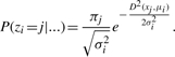
We introduce the missing data z = (z₁,…, z_N) in which z_i specifies a mixture cluster to the observation of x_i. Suppose that each z_i is a realization of a discrete random variable Z_i and that all Z_is (i = 1,…, N) are independent and identically distributed with the following probability mass function (pmf),

Conditional on the latent variable Z = (Z₁,…, Z_N) the data {x₁,…, x_N} are assumed to be independently observed from the density:

In our studies, we consider the situation in which the density f(x_i; μ_j, σ_j²) is a modified univariate Gaussian probability density function (pdf) with μ_j as the center of the cluster and σ_j² as the variance:

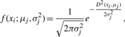where D(x_i, μ_j) denotes the distance between the sequence x_i and the center of the j-th cluster μ_j. We follow common approaches to assume a hierarchical model for the priors (with standard conjugacy):

where μ_i is chosen randomly from x₁,…, x_N without replacement. The final form of the prior probability is

and that of the posterior probability is

2.2 The birth–death process

To compute the parameters (π, μ, σ²) which maximize P(π, μ, σ²|x), we apply the MCMC method to construct an ergodic Markov Chain with the posterior distribution P(π, μ, σ²|x) as its stationary distribution. We design a Markov birth–death process as follows.

When the process is at a certain step t_i, and the number of existing clusters is k, the next step may be a ‘birth’ with a probability P_B/(P_B+P_D), or a ‘death’ with a probability P_D/(P_B+P_D), where P_B and P_D are the probability of a ‘birth’ and a ‘death’, respectively. P_B is given as a constant in our study, and P_D is defined as:

where d_i is the probability for a cluster to ‘die’. The way to compute d_i is shown in a later section.

Births: the (k+1)-th cluster is born with a new center μ_k+1 randomly chosen from x₁,…, x_N and μ_k+1≠μ_i (i = 1,…, k). The choice of μ_k+1 is based on the density:

where (μ_t, σ_t²) are the parameters of the cluster to which x_i is currently being assigned. Hence, μ_k+1 is preferred over those x_i's which are far away from the center of the cluster to which they currently belong. For other parameters of the new cluster, the priors are given as follows:

Then the existing parameters need to be updated (i = 1,…, k) by:

Deaths: an existing cluster dies independently of others with a probability

where L_−i indicates the likelihood without the i-th cluster and L indicates the likelihood with the i-th cluster:

Let N_c be the number of clusters. We use the Poisson distribution as its prior to simplify the form of d_i, as suggested by Stephens (2000):

Then we have a simplified form for the death probability d_i for each cluster:

We update π_j (j = 1,…, i−1, i+1,…, k) to reflect the death effect of the i-th cluster

For more details about the birth–death process, refer to (Stephens, 2000).

2.3 MCMC sampling

We update the parameters for the hierarchical mixture model in each step:

1. Update z by

   
2. Update π by

   

   where (n₁,…, n_k) are the numbers of data points belonging to individual mixture clusters. In other words, for j = 1,…, k,

   
3. Update σ² using the general approach as follows:

   

   Richardson and Stephens suggested another hierarchical level over β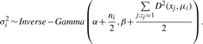

   

   where g and h are hyperparameters. However, as Richardson and Green (1997) mentioned, when applying the mixture model to the Bayesian classification, such update procedure would result in some clusters with a large variance, and its heavy tail would have a negative influence on the clustering result. This is because most methods assume that variances of clusters are similar to one another. Also, as mentioned before, restricting the variances is fundamental to obtain clustering results at different phylogenetic levels.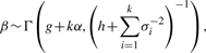
   In our method, we nested σ² by upper bound U and lower bound L. That is to say, if σ_i² < L or σ_i² > U, we would restart the updating procedure of σ_j² as indicated below:

   

   where β^′ is a given constant satisfying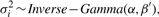

   

4. Update μ:

   Since μ is a vector of sequences chosen from data instead of a common numerical vector, we sample the center for each cluster in the following way.

For the j-th cluster, there are n_j sequences. Each n_j sequence is a potential candidate to be the center of this cluster. Let these sequences be X_j = {x_j1,…, x_jnj}. The likelihood of this cluster is defined as

where μ_j is the center of the cluster, σ_j² is the variance, and f is the Gaussian probability density function. Thus, for two candidate centers μ_j and μ_j^′, we have

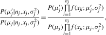which suggests a brute force method to sample the center sequence. Assume that

and then for each x_ji ∈ X_j, let δ_i denote the probability of choosing x_ji as the new center of this cluster

So we can define

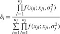and then sample a new center for each cluster.

2.4 Prior setting

Based on the priors suggested by Richardson and Green (1997) and Stephens (2000), with some minor modifications, we set

where R = Max–Min is the range of the data.

L and U, as the lower and upper bounds for variances, are determined by the different levels of accuracy to be achieved. For the dissimilarity threshold at roughly 3%, we suggest setting L = 1 and U = 2.25 (mentioned as clustering at ∼3% in later sections) so that the standard deviations of the Gaussian distributions in the mixture model will range from 1 to 1.5. For the threshold at 5%, we suggest setting L = 2.25 and U = 6.25 (mentioned as clustering at ∼5% in later sections) so that the standard deviations of Gaussian distributions in the mixture model will range from 1.5 to 2.5. It is the nature of Gaussian distribution that 95% of its density falls into the interval [μ − 2σ, μ + 2σ]. As such, the choice of Us, as noted above, virtually guarantees that at least 95% of the sequences in a given cluster will be <3% (if U = 2.25) or 5% (if U = 6.25) dissimilar from the center sequence in the cluster. At the same time, the choice of Ls, as noted above, helps to maintain the assumption that all Gaussian distributions in a mixture model will have similar variances. Under these circumstances, the settings suggested above for both Ls and Us should give results comparable with those of conventional hierarchical clustering methods that used 3 and 5% dissimilarity cutoffs, respectively. Although our approach is still associated with previously mentioned controversial 3 and 5% thresholds, it produces clusters with different standard deviations and its probabilistic nature fits better with real data. The settings of Ls and Us, as noted above, were used for all downstream analysis. Users can define their own Ls and Us in CROP.

2.5 Pairwise alignment and distance

The Needleman–Wunsch algorithm (Needleman and Wunsch, 1970) was used for pairwise alignment. However, we do not perform the dynamic programming on the whole matrix, only on a band near the diagonal with a width of 5% of the sequence length at each side. By doing this, we mainly focus on those sequence pairs with >90% similarity. The Quickdist algorithm (Sogin et al., 2006), which considers consecutive gaps in an alignment as one gap, is used to calculate the pairwise distance from the alignment results. Every distance is calculated as a percentage number in our approach. That is to say, a distance of 5.2 indicates 5.2% dissimilarity.

2.6 Computation

The most time-consuming part of Bayesian clustering is the pairwise alignment. The second most time-consuming part of the process involves updating centers, which is O(N²/k) (where N is the number of sequences and k is the number of clusters), whereas calculating the Gaussian probability density functions for all iterations and sequences is also a costive step. In order to improve the computational efficiency of Bayesian clustering, we introduce three operations, as noted below:

1. When the calculated dissimilarity D(x_i, x_j) between two sequences x_i and x_j is >15%, we set the Gaussian probability density function involving this distance to be 0. That is to say, we consider

   

   if D(x_i, x_j)≥ 15%.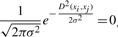
2. If the standard deviation of a cluster is σ_(t) and in next iteration, the updated value σ_(t+1) satisfies 0.9σ_(t) ≤ σ_(t+1) ≤ 1.1σ_(t), then for this cluster, we consider

   

   where μ is the center of this cluster and x is a sequence in this cluster.

3. Update all cluster centers if the current iteration gives birth to a new cluster; otherwise, we do not update centers. In addition, we do not update cluster centers for those clusters consisting of fewer than five sequences.

The first and second operations dramatically reduce the computational time for calculating the Gaussian pdfs, while the third operation avoids unnecessary updating of cluster centers. In practice, these operations do not compromise the accuracy of the results.

3 RESULTS

3.1 CROP work flow

Figure 1 shows a flowchart of CROP. First, the dataset is randomly split into blocks of 100–1000 sequences each. Generally, a smaller block size is preferred for longer sequences, such as full-length 16S rRNA gene sequences, while a larger block size is preferred for shorter sequences, such as one single hyper-variable region. Then, an independent Bayesian clustering is applied to each block. A distance matrix is generated for each block using the pairwise alignment algorithm. We run 20*(block size) iterations of MCMC, considering the first 10*(block size) iterations as burn-in. From all the iterations after burn-in, we choose the one with the largest posterior probability and report it as our clustering result for this block.

Fig. 1.

CROP workflow.

At the next level of the hierarchical approach, every cluster in each block is treated as one sequence with the center sequence as the representative, and all these center sequences are pooled and further split into blocks. However, a slightly different distance matrix is computed for each block. The matrix is a ‘center sequences against clusters’ matrix, in which the (i, j) entry indicates the distance between the i-th center sequence and the j-th cluster. We calculate this distance by the average distance between the i-th center sequence and C randomly chosen sequences from the j-th cluster (C = 20 is set for clusters with >20 sequences):

Finally, using this distance matrix, we apply a weighted Bayesian clustering on these clusters such that the weight is proportional to the size of the cluster, and this process will continue until one of the conditions noted below is satisfied.

1. The number of the clusters is >90% of the number of sequences. (This means most sequences are forming a cluster by themselves. Thus, split and merge process will not be able to reduce the dimension of the data efficiently any more.)

2. The number of the clusters is smaller than a predetermined threshold.

3. The process has been running for N times, where N is a predetermined threshold.

After the previous process, we will run one more round of Bayesian clustering on all the remaining clusters, and this result will constitute the final report. However, as a probabilistic approach, CROP may get slightly different results in different runs. Thus, in later sections, 10 runs were performed for all experiments, and the result with the highest posterior probability was chosen if not specified.

3.2 Estimating the number of OTUs

We first validated our method using a dataset described by Huse et al. (2007), which consisted of amplicons of V6 regions from 43 16S rRNA templates which were at least 3% different from each other. The sequenced reads were further categorized into two datasets. The first one (A) contained only those reads that were within 3% of one of the 43 templates, and the second dataset (B) contained all the reads. These two datasets consisted of 191 387 and 202 340 reads, respectively. To obtain the ground truth, we ran hierarchical clustering (using ESPRIT) on 43 template sequences. Then we compared CROP, ESPRIT and mothur (with and without the single linkage preclustering) using datasets (A) and (B) to obtain the number of OTUs. Default parameters were used for ESPRIT and mothur. For mothur, we used the same pairwise alignment program as implemented in ESPRIT to calculate a phylip format distance matrix and then specified the average linkage in clustering.

We ran the three programs on dataset (A) and the results were compared in Figure 2A. CROP identified 43 clusters when clustering at ∼3% (by using variance interval [1, 2.25], if unspecified). In 10 runs, CROP averaged 43.5±0.5 clusters, among which the result with 43 clusters gave the largest posterior probability. When clustering at ∼5% (by using variance interval [2.25, 6.25], if unspecified), CROP produced 42 clusters. In 10 runs, CROP averaged 43±0.8 clusters, among which the result with 42 clusters gave the largest posterior probability. Both results were in exact agreement with the ground truth.

Fig. 2.

Comparison of the number of OTUs predicted by CROP, ESPRIT and mothur (with and without single linkage preclustering) using two sequencing datasets generated from 43 16S rRNA templates (by Huse et al., 2007). Dataset (A) contains reads that are within 3% of the templates, and Dataset (B) contains all the raw reads.

To judge the accuracy of the predicted clusters, we compared cluster center sequences with the template sequences and assigned the cluster center with its most similar template sequence. We found that each template sequences, both at 3 and 5% thresholds, was uniquely assigned by a cluster center in ∼3 and ∼5% results, respectively, indicating 100% accuracy.

Then, we ran the three programs on the dataset (B). CROP identified 65 clusters when clustering at ∼3%. In 10 runs, CROP averaged 67.7±2.4 clusters. When clustering at ∼5%, the number of clusters decreased to 45, and averaged 45±1 in 10 runs. We also mapped the resulting center sequences to their nearest template sequences to access the accuracy of the results. In the ∼5% result, 43 out of 45 cluster centers were <5% dissimilar from their nearest template sequences, while the remaining 2 cluster centers were >10% dissimilar from their nearest templates. These two clusters were quite small, containing < 10 sequences. Similar observations were found for the ∼3% results where 43 out of 65 cluster centers were < 3% dissimilar from their nearest template sequences and each of the 43 template sequences is uniquely mapped by one of these 43 cluster centers, while the remaining 22 cluster centers were > 7% from their nearest template sequences and all of them are small (with < 10 sequences).

In comparison, CROP outperformed both ESPRIT and mothur, both of which overestimated the number of OTUs. As expected, mothur did a better job than ESPRIT when using the average linkage algorithm and the single linkage preclustering significantly improved the performance of the hierarchical clustering. However, in general, CROP is still more robust in dealing with sequencing errors and produces more accurate clustering results.

3.3 Validation results using a dataset of 90 artificial bacteria clones

We also obtained Quince's dataset (Quince et al., 2009) that consisted of 34 308 reads (12 360 unique reads) sequenced from V5 and V6 regions of 90 different clones of bacteria. This dataset contains very similar species (< 3% difference) and thus is appropriate for testing CROP's effectiveness on distinguishing closely related species. We applied CROP to this dataset using various intervals for the standard deviations of the Gaussian distributions. In addition to ∼3 and ∼5%, interval [0.2,0.5] was, for example, used to compare with the 1% dissimilarity threshold in hierarchical clustering, and interval [0.5,1] was, for example, used to compare with the 2% dissimilarity threshold in hierarchical clustering. The results were compared with the ground truth, as well as with those obtained from mothur (Schloss et al., 2009) with and without the single linkage preclustering (only unique reads used), and PyroNoise (Quince et al., 2009) followed by mothur. (The dataset was preprocessed with PyroNoise in order to reduce the noise in original data to improve the performance of hierarchical clustering in this case.) The input for mothur is the distance matrix we calculated using the pairwise alignment instead of the default multiple alignment. We chose the average linkage over the complete linkage in mothur, as the average linkage had been shown to produce better results by Quince et al. (2009).

As shown in Figure 3, mothur (preclustering) and PyroNoise (plus mothur) overestimated the number of OTUs. By mapping the cluster center sequences in CROP's result to the clusters in the result of PyroNoise's (plus mothur), we found that CROP achieved a result similar to that of PyroNoise's (plus mothur) at the regions with ≥ 2% dissimilarity in terms of the number of clusters and cluster contents detected. However, as the threshold decreased, especially at ≤1% dissimilarity regions, CROP did overestimate the number of OTUs because the sequencing error rate was around 1%. The single linkage preclustering slightly improved the performance of the hierarchical clustering. Although the improvement was not as significant as the previous case, it did reduce the number of sequences to be clustered from 12 360 to 5370, and thus could be still helpful in dealing with large datasets. In general, CROP achieved a performance similar to that of PyroNoise (plus mothur) at 5 and 3% and did so using significantly less computational time and without modeling the sequencing errors. PyroNoise alone used more than 1 day on cluster computers with 128 CPUs to process these datasets as reported by the study, while CROP completed the work within 3 h using a single CPU.

Fig. 3.

Comparison of the number of OTUs found by CROP, PyroNoise (plus mothur) and mothur, in which the results for CROP are shown both as a straight dashed line indicating the number of OTUs when using different parameters and as an approximated average lineage-through-time curve (CROP Assumption).

3.4 Estimating abundance levels of clusters using the human skin microbiome dataset

In this application, we applied CROP to the human skin microbiome data by Grice et al. (2009). We first chose a skin site, the axillary vault (AV) of patient HV5 consisting of 1130 nearly full-length 16S rRNA sequences. Then we used the ribosomal database project (RDP) classifier (Cole et al., 2009) to infer the taxonomy for each sequence. These results were considered to be the ground truth in this experiment. According to this ground truth, we found that the original result (Grice et al., 2009) underestimated the abundance of the genus Propionibacteria. Then we applied CROP to cluster this dataset at ∼5%. To compare our clustering results with the ground truth, we assigned genera to each cluster by searching the center sequence in the RDP database. CROP identified 34 clusters. Figure 4A shows that our results are very similar to the ground truth and that among the 33 detected genera in the ground truth, 32 are uniquely mapped by 32 clusters in our results. The only difference between our results and the ground truth occurs in the class Actinobacteria, where four sequences belonging to the genus Williamsia are assigned to the genus Mycobacterium and Corynebacterium (Fig. 4B). All three of these genera are in the same suborder Corynebacterineae. In comparison, mothur (using the average linkage) produces 47 clusters, overestimating the number of genera by 43%.

Fig. 4.

The clustering results (by CROP) of the human microbial sequencing data at the AV skin location: (A) ∼5% results and the ground truth and (B) more detailed results inside the ‘Other Actinobacteria’.

3.5 Comparing different microbial communities using the human skin microbiome dataset

Finally, we applied CROP to three human skin microbiome datasets: sebaceous (including glabella, alar crease, external auditory canal, occiput, manubirum and back), moist (including nare, AV, antecubital fossa, interdigital web space, inguinal crease, gluteal crease, popliteal fossa, plantar heel and umbilicus) and dry (including volar forearm, hypothenar palm and buttock). After clustering, every cluster center was searched against the RDP database to determine the taxonomy of this cluster. The results are shown in Supplementary Figure 1. Betaproteobacteria is shown to dominate the dry locations, while Corynebacteria and Propionibacteria, both belonging to Actinobacteria, are shown to dominate the moist and sebaceous locations, respectively.

To study the species similarity and difference between different skin locations, while also to validate CROP at species level using real environmental data, we merged all sequences, clustered them using CROP at ∼3%, and computed the Jaccard index value and the Theta index value (Grice et al., 2009) to see if we got consistent species-level result with previous studies. The Jaccard index value measures the sample membership by the proportion of shared OTUs between the two samples. The Theta index value measures the sample structure by taking OTU abundance levels into consideration. Basically, the similarity of the two samples tends to increase as both Jaccard and Theta index values increase. These results show that the Jaccard index values of the two skin locations with the same environmental conditions (dry, moist or sebaceous) were not significantly different from those with different environmental conditions (P = 0.53, two-sided t-test); however, the Theta index values did show significant differences (P = 2.33 × 10⁻²⁵, two-sided t-test). These results suggest that the environmental conditions might not significantly affect the composition of the bacterial communities located on the human skin, but they could instead affect the relative abundance levels. The pairwise Theta index values between skin locations are shown in Figure 5B. Using these pairwise Theta index values as a distance measure, we clustered these 18 skin locations using hierarchical clustering (Fig. 5A). The figure shows that skin locations are not clustered together strictly following their environmental conditions. For example, the antecubital fossa and the interdigital web space, both moist, are more similar to the volar forearm and the hypothenar palm, both dry, than to each other. Thus, it appears most likely that a spatial relationship dominates the environmental conditions in these cases, as all four skin locations are found on the human forearms. It might therefore be concluded that environments and locations on the human body co-determine the human microbiome distribution, a theory which agrees with what was found in another human skin microbiome study (Costello et al., 2009).

Fig. 5.

The Theta index values and the phylogenetic tree constructed based on these values. (A) Phylogenetic tree of 18 human skin locations with their environmental conditions annotated in brackets. (B) Theta index values shown as a heatmap.

Rarefaction curves for each of the three types of skin locations are drawn in Figure 6, showing that the sebaceous locations are less diverse than the moist or dry locations with respect to the number of OTUs. These conclusions are consistent with a previous study (Grice et al., 2009). Results from mothur (with preclustering, pairwise alignment and the average linkage) are also shown in Figure 6 for comparison. Hierarchical clustering still overestimates the number of OTUs.

Fig. 6.

The rarefaction curves for all three human skin types.

4 DISCUSSION

CROP provides a clustering tool that automatically determines the best clustering result for 16S rRNA sequences at different phylogenetic levels. Yet, at the same time, it is able to manage large datasets and to overcome sequencing errors. Our study shows that CROP gives accurate clustering results, both in terms of the number of clusters and their abundance levels, for various types of 16S rRNA datasets. In contrast, the standard hierarchical clustering strategy, even with the preclustering process and the average linkage method, still frequently overestimates the number of OTUs in the presence of sequencing errors, resulting in an underestimation of the abundance level of the underlying OTUs. In addition, we demonstrate by using the human skin dataset that the results produced by CROP can provide compelling biological insights into different microbial communities.

REFERENCES

- Brown DP. Efficient functional clustering of protein sequences using the Dirichlet process. Bioinformatics. 2008;24:1765–1771. doi: 10.1093/bioinformatics/btn244. [DOI] [PubMed] [Google Scholar]
- Cole JR, et al. The ribosomal database project: improved alignments and new tools for rRNA analysis. Nucleic Acids Res. 2009;37:D141–145. doi: 10.1093/nar/gkn879. [DOI] [PMC free article] [PubMed] [Google Scholar]
- Costello EK, et al. Bacterial community variation in human body habitats across space and time. Science. 2009;326:1694–1697. doi: 10.1126/science.1177486. [DOI] [PMC free article] [PubMed] [Google Scholar]
- DeSantis TZ, Jr, et al. NAST: a multiple sequence alignment server for comparative analysis of 16S rRNA genes. Nucleic Acids Res. 2006;34:W394–W399. doi: 10.1093/nar/gkl244. [DOI] [PMC free article] [PubMed] [Google Scholar]
- Eisen JA. Environmental shotgun sequencing: its potential and challenges for studying the hidden world of microbes. PLoS Biol. 2007;5:e82. doi: 10.1371/journal.pbio.0050082. [DOI] [PMC free article] [PubMed] [Google Scholar]
- Enright AJ, et al. An efficient algorithm for large-scale detection of protein families. Nucleic Acids Res. 2002;30:1575–1584. doi: 10.1093/nar/30.7.1575. [DOI] [PMC free article] [PubMed] [Google Scholar]
- Grice EA, et al. Topographical and temporal diversity of the human skin microbiome. Science. 2009;324:1190–1192. doi: 10.1126/science.1171700. [DOI] [PMC free article] [PubMed] [Google Scholar]
- Huse SM, et al. Accuracy and quality of massively parallel DNA pyrosequencing. Genome Biol. 2007;8:R143. doi: 10.1186/gb-2007-8-7-r143. [DOI] [PMC free article] [PubMed] [Google Scholar]
- Huse SM, et al. Ironing out the wrinkles in the rare biosphere through improved OTU clustering. Environ. Microbiol. 2010;12:1889–1898. doi: 10.1111/j.1462-2920.2010.02193.x. [DOI] [PMC free article] [PubMed] [Google Scholar]
- Johnson SC. Hierarchical clustering schemes. Psychometrika. 1967;32:241–254. doi: 10.1007/BF02289588. [DOI] [PubMed] [Google Scholar]
- Katoh K, et al. MAFFT version 5: improvement in accuracy of multiple sequence alignment. Nucleic Acids Res. 2005;33:511–518. doi: 10.1093/nar/gki198. [DOI] [PMC free article] [PubMed] [Google Scholar]
- Marco D. Metagenomics: Theory, Methods and Applications. Norwich: Caister Academic Press; 2010. [Google Scholar]
- Marttinen P, et al. Bayesian search of functionally divergent protein subgroups and their function specific residues. Bioinformatics. 2006;22:2466–2474. doi: 10.1093/bioinformatics/btl411. [DOI] [PubMed] [Google Scholar]
- Needleman SB, Wunsch CD. A general method applicable to the search for similarities in the amino acid sequence of two proteins. J. Mol. Biol. 1970;48:443–453. doi: 10.1016/0022-2836(70)90057-4. [DOI] [PubMed] [Google Scholar]
- Quince C, et al. Accurate determination of microbial diversity from 454 pyrosequencing data. Nat. Methods. 2009;6:639–641. doi: 10.1038/nmeth.1361. [DOI] [PubMed] [Google Scholar]
- Richardson S, Green PJ. On Bayesian analysis of mixtures with an unknown number of components. J.R. Stat.Soc. Ser. B (Methodol.) 1997;59:731–792. [Google Scholar]
- Rothberg JM, Leamon JH. The development and impact of 454 sequencing. Nat. Biotechnol. 2008;26:1117–1124. doi: 10.1038/nbt1485. [DOI] [PubMed] [Google Scholar]
- Schloss PD. The effects of alignment quality, distance calculation method, sequence filtering, and region on the analysis of 16S rRNA gene-based studies. PLoS Comput. Biol. 2010;6:e1000844. doi: 10.1371/journal.pcbi.1000844. [DOI] [PMC free article] [PubMed] [Google Scholar]
- Schloss PD, Handelsman J. Introducing DOTUR, a computer program for defining operational taxonomic units and estimating species richness. Appl. Environ. Microbiol. 2005;71:1501–1506. doi: 10.1128/AEM.71.3.1501-1506.2005. [DOI] [PMC free article] [PubMed] [Google Scholar]
- Schloss PD, et al. Introducing mothur: open-source, platform-independent, community-supported software for describing and comparing microbial communities. Appl. Environ. Microbiol. 2009;75:7537–7541. doi: 10.1128/AEM.01541-09. [DOI] [PMC free article] [PubMed] [Google Scholar]
- Sogin ML, et al. Microbial diversity in the deep sea and the underexplored “rare biosphere”. Proc. Natl Acad. Sci. USA. 2006;103:12115–12120. doi: 10.1073/pnas.0605127103. [DOI] [PMC free article] [PubMed] [Google Scholar]
- Stephens M. Bayesian analysis of mixture models with an unknown number of components - an alternative to reversible jump methods. Ann. Stat. 2000;28:40–74. [Google Scholar]
- Sun Y, et al. ESPRIT: estimating species richness using large collections of 16S rRNA pyrosequences. Nucleic Acids Res. 2009;37:e76. doi: 10.1093/nar/gkp285. [DOI] [PMC free article] [PubMed] [Google Scholar]
Associated Data
This section collects any data citations, data availability statements, or supplementary materials included in this article.