Measuring Retroactivity from Noise in Gene Regulatory Networks

Abstract

Synthetic gene regulatory networks show significant stochastic fluctuations in expression levels due to the low copy number of transcription factors. When a synthetic gene network is allowed to regulate a downstream network, the response time of the regulating transcription factors increases. This effect has been termed “retroactivity”. In this article, we describe a method for estimating the retroactivity of a given system by measuring the stochastic noise in the transcription factor expression. We show that the noise in the output signal of the network can be affected significantly when the output is connected to a downstream module. More specifically, the output signal noise can show significantly longer correlations. We define retroactivity by the change in the correlation time. This measure of retroactivity corresponds well to the deterministic retroactivity described in another study. We provide an estimation method for measuring retroactivity from the gene expression noise by investigating its autocorrelation function. When retroactivity is defined using the decay (correlation) times from the gene expression autocorrelation functions, it is found not to depend on whether the module output is defined as either the free transcription factor or the total of the bound and free transcription factor. The frequency domain response, however, depends strongly on which output variable is considered. The proposed estimation method for measuring retroactivity, based on the gene expression noise, can serve as a practical method for characterizing interface conditions between two synthetic modules and eventually provide a step toward large-scale circuit design for synthetic biology.

Introduction

In synthetic biology, independent or modular units are crucial to the design process when building a gene network from individually characterized modules (1–5). A module-based approach can provide an efficient information exchange due to the reusability of previously-designed and experimentally-tested modules. The approach can also provide predictable design of global behavior based on each individually characterized module. Because of these merits, synthetic biologists have been promoting the idea of modularity in diverse directions, for example: bioinformatics (6), software engineering (7), experiments, and theoretical approaches.

Del Vecchio et al. (8) introduced a measure called “retroactivity” that allows one to determine the influence a downstream module has on the characteristics of an upstream module. The higher the retroactivity, the greater the influence from the downstream module and the less modular the functional upstream units. More specifically, they considered a gene network (which we call a circuit) whose outputs are transcription factors (TFs) that can regulate specific promoters on a downstream module (see Fig. 1). They showed that the upstream module output responds much more slowly when it regulates a downstream module than for the case when the output is isolated (8), and that this slowdown in the output kinetics can affect the dynamics of the upstream module.

Figure 1.

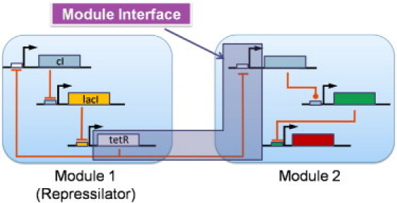
Module interface process: Module 1, representing the repressilator (22), regulates Module 2. One of the transcription factors of the repressilator, TetR, is chosen as an output of Module 1 and TetR-specific promoters in Module 2 as an input of Module 2. The interface process between the two modules represents tetR transcription, translation, and its regulation on the promoters in Module 2.

In this article, we focus on an operational method for measuring the retroactivity by using the stochastic nature of gene circuits. Gene expression is known to show significant stochastic fluctuations (9–16) (for review (17–20)), which often contains useful information that is not available by simply observing the mean values (21). Because the noise can be considered an outcome of continuous perturbations (generated from both intrinsic and extrinsic sources), it can be used to obtain the systems dynamical response to the perturbations. In this article, we investigate the measurable changes in the statistics of the noise due to connections between gene circuit components and propose a practical method to measure retroactivity to quantify the level of modularity in circuit components.

Materials and Methods

Gene expression models and autocorrelation functions

In this section, we present a stochastic model of gene expression for transcription factors (TFs), taking into account retroactivity due to binding-unbinding interactions between the TFs and their specific promoter region. We aim to describe the dynamics of the processes in the slow timescale, where we assume the binding-unbinding processes of the TFs to be in equilibrium. In the slow timescale, the dynamics can be described by a slow variable, the total number X_tot of TFs. To derive the autocorrelation function, we consider the dynamical response of the noise component of X_tot: δX_tot. Because our simulations show that its autocorrelation can be approximated as a pure exponential function (when the extrinsic noise is not considered), we assume that δX_tot shows a single response time T and model the process by the following Langevin equation,

$$\frac{d\delta X_{tot}}{dt}=-{\gamma }_I\delta X_{tot}+I,$$ (1)

where γ_I ≡ 1/T and I represents intrinsic noise which is exponentially correlated (14–16) as

$$\langle I\left(t\right)I\left(t+\tau \right)\rangle =W_I\exp \left(-\tau /T_I\right),$$

where the angle bracket denotes an average over a time series at the stationary state and T_I denotes the correlation time of intrinsic noise. When the extrinsic noise is considered, the model process can be modified as

$$\frac{d\delta X_{tot}}{dt}=-\left({\gamma }_I+{\gamma }_E\right)\delta X_{tot}+I+E,$$ (2)

where γ_E is given by log(2)/T_d with T_d cell doubling time and E represents extrinsic noise satisfying (14–16)

$$\langle E\left(t\right)E\left(t+\tau \right)\rangle =W_E\exp \left(-\tau /T_E\right),$$

where T_E denotes the correlation time of extrinsic noise (later we will assume that γ_E is equal to 1/T_E).

An autocorrelation function (22) (for gene expression studies (13–16)) quantifies the correlation of the signal (X_tot) with itself for a given time-lag (τ):

$$G_{X_{tot}}\left(\tau \right)=\langle \left(X_{tot}\left(t+\tau \right)-\langle X_{tot}\rangle \right)\left(X_{tot}\left(t\right)-\langle X_{tot}\rangle \right)\rangle ,$$ (3)

where X_tot(t) is the signal amplitude at time t and is presumed at a stationary state fluctuating with respect to a constant mean. This autocorrelation function has been experimentally measured to understand the noise power spectrum in gene expression levels of a HIV transcriptional circuit (15) and TetR negative feedback circuit (14). Autocorrelation has also been used to investigate the properties of intrinsic and extrinsic noise (13) and to analyze regulatory interactions in a CRP-GalS-GalE feed-forward circuit (16). Here we offer a new (to our knowledge) application of autocorrelation functions in relation to the analysis of modularity.

To obtain the autocorrelation function of X_tot, we obtain the integral-type solution of Eq. 2 for X_tot(t) and substitute the solution into Eq. 3, resulting in

$$G_{X_{tot}}\left(\tau \right)=\frac{W_I/T_I}{{\left(1/T_I\right)}^2-{\gamma }^{\prime 2}}\left(-\frac{e^{-\tau /T_I}}{1/T_I}+\frac{e^{-{\gamma }^{\prime }\tau }}{{\gamma }^{\prime }}\right)+\frac{W_E/T_E}{{\left(1/T_E\right)}^2-{\gamma }^{\prime 2}}\left(-\frac{e^{-\tau /T_E}}{1/T_E}+\frac{e^{-{\gamma }^{\prime }\tau }}{{\gamma }^{\prime }}\right),$$ (4)

with γ′ ≡ γ_I + γ_E.

We will show that the above autocorrelation function, Eq. 4, is consistent with the functional forms obtained or used in the literature (13,14,16). To show the consistency with Austin et al. (14), we consider that the internal noise correlation time is much smaller than the extrinsic noise correlation time (i.e., T_I ≪ T_E) and that the time interval τ is much larger than T_I. Under the assumption that γ_E = 1/T_E, we can simplify the above equation to Eq. 13, giving an identical result presented in Austin et al. (14). In Rosenfeld et al. (13) and Dunlop et al. (16), the authors did not use degradation-tagged TFs in measuring their expression levels, so the lifetimes of the TFs were much larger than the cell doubling time (γ_I ≪ γ_E and thus γ′ ≃ γ_E). The authors assumed that γ_E = 1/T_E. In this case, the autocorrelation can be simplified to (13,16) $A^{\prime }\exp \left(-\tau /T_I\right)+B^{\prime }\exp \left(-\tau /T_E\right).$

Reaction models for X_tot

We justify the stochastic reaction processes described in Fig. 2, C and D. We construct the master equation for X_tot and P_b:

$$\frac{\partial P\left(X_{tot},P_b;t\right)}{\partial t}=P\left(X_{tot}-1,P_b\right)\alpha +P\left(X_{tot},P_b-1\right)k_{on}\left(P_t-P_b+1\right)\left(X_{tot}-P_b+1\right)+P\left(X_{tot}+1,P_b\right)\gamma \left(X_{tot}+1-P_b\right)+P\left(X_{tot},P_b+1\right)k_{off}\left(P_b+1\right)-P\left(X_{tot},P_b\right)\left[\alpha +\gamma \left(X_{tot}-P_b\right)+k_{off}{P}_b+k_{on}\left(P_t-P_b\right)\left(X_{tot}-P_b\right)\right],$$

where P(X_tot, P_b; t) is the probability to find X_tot total TFs and P_b bound TFs at time t. This justifies the reaction model for X_tot shown in Fig. 2 C is exact at the master equation level.

Figure 2.

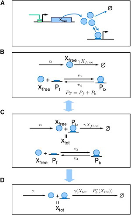
Reaction models for a module interface process: (A) Monomer transcription factors (output of an upstream module) regulate promoters located in a downstream module. (B) This interface process is modeled by TF translation, degradation, and binding-unbinding processes. The copy number of unbound TFs, unbound promoters, and bound promoters are denoted by X_free, P_f, and P_b, respectively. P_T is the total number of promoters. This reaction model can be equivalently described by panel C. X_tot denotes the total copy number of the TFs. (D) The reaction model from panels B and C can be simplified under the quasiequilibrium assumption for P_b. The full model from panel B is used for simulations and the approximate model from panel D is introduced for formulating the concept of stochastic retroactivity (not for simulations).

As in the deterministic case, we assume the transcription factor binding-unbinding process is in a quasiequilibrium state for a given value of X_tot (γ ≪ k_on X_free + k_off; see (8,23,24)),

$$P\left(X_{tot},P_b;t\right)=P\left(P_b|X_{tot}\right)P\left(X_{tot};t\right),$$

where P(P_b |X_tot) is the probability distribution function of P_b for a given value of X_tot at the quasiequilibrium (17). This approximation simplifies the above equation to another master equation for the slow variable X_tot:

$$\frac{\partial P\left(X_{tot};t\right)}{\partial t}=\alpha \left[P\left(X_{tot}-1;t\right)-P\left(X_{tot};t\right)\right]+\gamma \left(X_{tot}+1-{\langle P_b\rangle }_{X_{tot}+1}\right)P\left(X_{tot}+1;t\right)-\gamma \left(X_{tot}-{\langle P_b\rangle }_{X_{tot}}\right)P\left(X_{tot};t\right).$$

For the fast mode process, we use the quasiequilibrium assumption, specifically the detailed balance:

$$k_{off}\left(P_b+1\right)P\left(P_b+1|X_{tot}\right)=k_{on}\left(P_T-P_b\right)\left(X_{tot}-P_b\right)P\left(P_b|X_{tot}\right).$$

From the detailed balance we obtain the equilibrium probability distribution function P(P_b |X_tot) of P_b and then obtain the average copy number of the bound transcription factor, ${\langle P_b\rangle }_{X_{tot}}$:

$${\langle P_b\rangle }_{X_{tot}}=\sum _{P_b=0}^{X_{tot}}{\left(\frac{k_{on}}{k_{off}}\right)}^{P_b}\frac{P_T!X_{tot}!}{\left(P_b-1\right)!\left(P_t-P_b\right)!\left(X_{tot}-P_b\right)!}P\left(0|X_{tot}\right).$$ (5)

By using Eq. 5, we replace P_b^∗ appearing in the degradation rate function of X_tot in the deterministic case, to ${\langle P_b\rangle }_{X_{tot}}$. This means that the slow process can be simplified to the reaction process shown in Fig. 2 D.

Deterministic retroactivity for a module interface process involving dimer TFs

This section shows the derivation of the deterministic retroactivity for the module interface process described in the example “Dimer transcription factor with negative feedback,” by obtaining a response time. The total transcription factor (monomer units) (X_tot = X + 2X₂ + 2P_b) evolves in time by following

$$\frac{d{X}_{tot}}{dt}=\alpha \left(X_2\right)-\gamma X-2{\gamma }_2{X}_2,$$

with

$$\alpha \left(X_2\right)\equiv \frac{\alpha }{1+\beta X_2}.$$

The response time constant of X_tot becomes

$$\begin{array}{c}{T}_c=-{\left[\frac{d}{d{X}_{tot}}\left(\alpha \left(X_2\right)-\gamma X-2{\gamma }_2{X}_2\right)\right]}^{-1}\\ ={\left[\frac{-d\alpha \left(X_2\right)}{dX}\frac{dX}{d{X}_{tot}}+\gamma \frac{dX}{d{X}_{tot}}+2{\gamma }_2\frac{d{X}_2}{d{X}_{tot}}\right]}^{-1}.\end{array}$$ (6)

Under the assumption of the equilibrium of X₂ and P_b, we obtain

$$\begin{array}{l}{X}_2=\frac{k_1}{k_2+{\gamma }_2}{X}^2,\hfill \\ P_b=\frac{P_T{X}_2}{K_d+X_2}\equiv P_{T}f\left(X\right),\hfill \end{array}$$ (7)

where we replace the reaction rate of dimerization to k₁X² for simplicity. By substituting the first equation in the above to Eq. 6, the time constant is obtained as

$$T_c={\left[-\frac{d\alpha \left(X_2\right)}{dX}+\gamma +\frac{4{\gamma }_2{k}_{1}X}{k_2+{\gamma }_2}\right]}^{-1}\frac{d{X}_{tot}}{dX},$$

which becomes, by using X_tot = X + 2X₂ + 2P_b and Eq. 7,

$$T_c=T_i\left[1+\frac{2f^{\prime }\left(X\right)}{1+\frac{4k_{1}X}{k_2+{\gamma }_2}}{P}_T\right],$$ (8)

where T_i denotes the time constant in the isolated case,

$$T_i=\frac{1+\frac{4k_{1}X}{k_2+{\gamma }_2}}{-\frac{d\alpha \left(X_2\right)}{dX}+\gamma +\frac{4{\gamma }_2{k}_{1}X}{k_2+{\gamma }_2}}.$$

Here the concentration levels of X and X₂ are independent of P_T at the stationary state. The retroactivity is obtained by using Eq. 10.

Software

All stochastic simulations were carried out using our own Gillespie code written in C and run on a Quad-core PC under the Ubuntu LINUX OS. Deterministic simulations were carried out using the software SBW (25,26).

Results

Module interface process

We begin by defining the term, module interface process (MIP), as a collection of reactions involving upstream-module TFs that regulate downstream-module promoters. For example, consider a synthetic oscillator such as a repressilator (27) and one of the TFs, TetR, where TetR is allowed to regulate promoters located in its downstream module as shown in Fig. 1. Here the MIP represents tetR transcription, translation, and regulation (binding-unbinding) of the downstream promoters.

Deterministic retroactivity

We will first review the work by Del Vecchio et al. (8) on retroactivity in gene-regulatory networks. They considered a simple MIP shown in Fig. 2 A and modeled it as a reaction process described in Fig. 2 B, where they assumed that the degradation of bound TFs is negligible compared to that of free TFs. The total number of TFs (free and bound) denoted by X_tot can fluctuate only when the TFs are translated or degraded. Thus, the MIP can be equivalently described as in Fig. 2 C. Del Vecchio et al. also assumed that the binding-unbinding reactions are fast enough that the number of the bound TFs denoted by P_b is in quasiequilibrium:

$$k_{on}{X}_{free}{P}_f=k_{off}{P}_b.$$

By using this equation, we can express P_b in terms of X_tot:

$$P_b^{\ast }\left(X_{tot}\right).$$

Then the MIP can be simplified as shown in Fig. 2 D.

The degradation rate of X_tot in the MIP (γ(X_tot – P_b^∗ ); see Fig. 2 D) was shown to be highly nonlinear in X_tot (see Fig. 3) (8,28), and this nonlinearity was understood from the continuous sequestration of X_free to a nondegradable state (P_b) (28). That is, when the copy number of the total TFs is much larger than that of the specific promoters, most of the TFs are found to be unbound, i.e., in the degradable state. Mathematically the degradation rate of X_tot is approximated as

$$\gamma \left(X_{tot}-P_b^{\ast }\right)\simeq \gamma X_{tot}$$

as shown in Fig. 3 B. However, if the copy number of the total TFs and their promoters are in the same order of magnitude, most of the TFs become bound to the promoter regions (when the TF-promoter affinity is strong), i.e., in the nondegradable state. Thus, the net degradation rate of the total TFs becomes significantly reduced.

Figure 3.

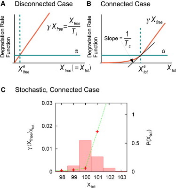
Degradation rate functions (γX_free) for the module interface process shown in Fig. 2D. In the deterministic framework (A and B), $X_{free}^e$and $X_{tot}^e$ represent the concentrations of the transcription factor at equilibrium. In the connected case, the degradation rate becomes ∼γX_tot for sufficiently large X_tot. In the stochastic framework (C), the degradation rate function $\gamma {\langle X_{free}\rangle }_{X_{tot}}$ can become highly nonlinear for the probable region of X_tot. The average copy number of the unbound TFs ${\langle X_{free}\rangle }_{X_{tot}}$ is computed for the different values of the total copy number (X_tot) by using Eq. 5, and the probability distribution function of X_tot, P(X_tot), is numerically computed for the process shown in Fig. 2D based on the Gillespie stochastic simulation algorithm (35). Parameters: K_d = 1 pM and P_T = 100 nM [α = 0.5 nM h⁻¹, γ = 1 h⁻¹, k_on = 10 nM⁻¹ h⁻¹, and k_off = 0.01 h⁻¹]. We set the volume of the host cell (e.g., E. coli) roughly equal to 1 μm³, and a copy number of one corresponds to 1 nM. As a result, we interchange the unit of nM with that of copy number.

This nonlinear degradation rate of X_tot causes the dynamics of the upstream module output to slow down. To quantify the slowdown, Del Vecchio et al. (8) introduced a measure called “retroactivity”. The speed of the dynamics, more specifically the speed of the response to a perturbation in X_tot, is related to how quickly the degradation rate changes to buffer the perturbation: The response time is inversely proportional to the slope of the degradation rate function (Fig. 3 B). When the equilibrium state is perturbed, the response time T_c is expressed as

$$\frac{1}{T_c}\equiv {\frac{d}{d{X}_{tot}}\left[\gamma \left(X_{tot}-P_b^{\ast }\right)\right]|}_{X_{tot}=X_{tot}^e}={\gamma \left(1-\frac{d{P}_b^{\ast }}{d{X}_{tot}}\right)|}_{X_{tot}=X_{tot}^e},$$

with X^e_tot the equilibrium value of X_tot. The term appearing in the above, dP_b^∗/dX_tot, was defined as the retroactivity and shown to be between 0 and 1 (8). Thus, the response time T_c in the connected case becomes larger than the response time T_i (≡ 1/γ) of the isolated case. Retroactivity estimated in this deterministic framework (8) will be henceforth called the deterministic retroactivity (d-retroactivity).

Stochastic retroactivity

In this section, we consider the MIP described in Fig. 2 B in the stochastic regime. The value of P_b fluctuates stochastically. There are two types of fluctuations, fast and slow. The fast one comes from the rapid binding-unbinding reactions and the other from the slow translation-degradation processes. We are interested in the timescale of the slow process and assume quasiequilibrium in the binding-unbinding processes. At the first level approximation, we replace P_b^∗ with the mean value of P_b over the fast fluctuations (refer to the Materials and Methods).

Consider first the isolated case. In the stochastic description, stochastic fluctuations in X_free, deviating from the stationary-state mean value will spend a time 1/γ typically in reaching the mean value (Fig. 4). The autocorrelation function $G_{X_{free}}\left(\tau \right)$ (for a definition see the Materials and Methods) becomes significant up to the time interval 1/γ (called the correlation time; see Fig. 4): mathematically (22),

$$G_{X_{free}}\left(\tau \right)=G_{X_{free}}\left(0\right)e^{-\tau /T_i}\text{with}{T}_i\equiv 1/\gamma .$$

For the isolated case, the correlation time in the stochastic framework equals the response time in the deterministic framework (22).

Figure 4.

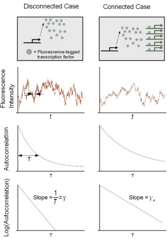
Stochastic fluctuations in a fluorescence signal (X_tot(t)) from fluorescence-tagged TFs: If the autocorrelation function of X_tot(t) follows an exponential function $G_{X_{tot}}\left(\tau \right)=G_{X_{tot}}\left(0\right)e^{-\frac{\tau }{T}}$, the correlation time corresponds to T (22). The autocorrelation can show longer correlations when the upstream module regulates the downstream one and causes the correlation time to increase.

For the connected case, the correlation time will be shown to increase when compared with the isolated case. Consider the case of the nonlinear degradation shown in Fig. 3 C. Most of the fluctuations in the total copy number, X_tot, occur between 99 and 102. Among them, the fluctuations between 100 and 102 will have a correlation time ≃ 1/γ (inverse of the slope of the degradation rate function), whereas those between 99 and 100 will have a correlation time much larger than 1/γ. Thus, the net correlation time increases, reflecting the increase in the response time in the deterministic framework, i.e., retroactivity.

We can investigate how to define the retroactivity in the stochastic framework (named stochastic retroactivity or s-retroactivity). The stochastic fluctuations in X_tot can be centered around the nonlinear region of the degradation rate function (as shown in Fig. 3 C) such that the discreteness of X_tot needs to be carefully taken into account. In such a case, we cannot make a clear mathematical definition of retroactivity, because the derivative of the degradation rate function with respect to X_tot is not well defined. Instead, we define the retroactivity (R_s) from the change in the correlation times between the isolated and connected cases. The correlation time T is measured from the slope of $\log G_{X_{tot}}\left(\tau \right)$ (note for the isolated case that X_tot = X_free):

$$1/T\equiv -\frac{d\log G_{X_{tot}}\left(\tau \right)}{d\tau }.$$ (9)

The retroactivity is defined as

$$R_s\equiv \frac{T_c-T_i}{T_c},$$ (10)

where T_c denotes the correlation time in the connected case and T_i, in the isolated case.

We have numerically estimated the stochastic retroactivity by performing stochastic simulations. We have used parameter values appropriate for degradation-tagged TFs in E. coli host cells: The average copy number of the TF is set equal to 2, the dissociation constant of the TF specific promoters is set between 0.001 and 100 nM (13,29–31), and the average copy number of plasmids containing the specific promoters is set to 1 and 100 (for the reaction parameter values, refer to the caption of Fig. 5). We have set the volume of E. coli roughly equal to 1 μm³, and for this volume, a copy number of 1 corresponds to 1 nM. Hereafter we will interchange the unit of nM with that of a copy number. We have fitted the autocorrelation to an exponential function. The measured s-retroactivity is shown to be well matched with the d-retroactivity (R_d), as shown in Fig. 5, A and B. This result implies that the d-retroactivity can be used to estimate retroactivity for the case when stochastic fluctuations are significant, e.g., the case of low copy number TFs.

Figure 5.

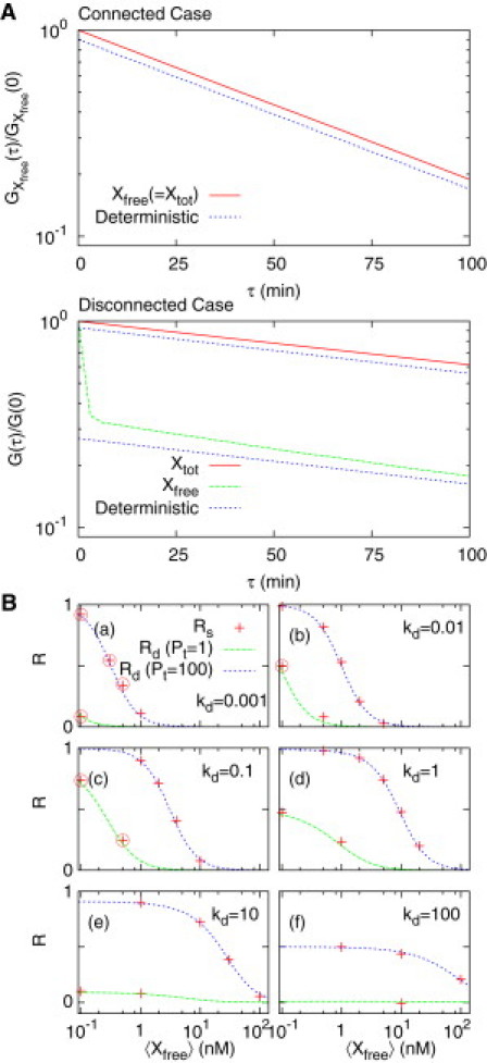
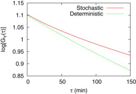
Retroactivity in the stochastic and deterministic cases: (A) For the connected case modeled as in Fig. 2B, the autocorrelation function of the total TF concentration (X_tot) approximates an exponential function and its correlation time also approximates the response time measured in the deterministic case. However, the approximation does not hold well for the autocorrelation of unbound TF (X_free) and its correlation time. This is due to an interfering effect from the fast reactions of TF binding/unbinding. The lines labeled “Deterministic” are drawn for comparison purposes. (B) For various parameter values that are experimentally reasonable, we measure the retroactivities (R_s) from the autocorrelations of X_tot by performing stochastic simulations. The retroactivities R_s approximate the deterministic estimates R_d. In the circled cases in panel B, the autocorrelation of X_tot could not be approximated as an exponential function and the retroactivities were obtained from the slope corresponding to a small τ-region [0, 25 ∼ 50] (see the Discussion and Fig. 9). The unit of K_d is nM. We used the Gillespie stochastic simulation algorithm (35). Parameters: (A) K_d = 0.1 nM with k_on = 10 nM⁻¹ h⁻¹, 〈X_free〉 = α/γ = 2 nM (α = 2 nM h⁻¹, γ = 1 h⁻¹), and P_T = 100 nM. (B) γ = 1 h⁻¹, k_on = 10 nM⁻¹ h⁻¹ (12).

Retroactivity: relative decrease in the cutoff frequency of a MIP

In this subsection, we will make a connection between the retroactivity and frequency response of a gene circuit. Retroactivity will be shown to be related to the change in the cutoff frequency of a MIP due to the downstream module regulation. The cutoff frequency is defined in the deterministic framework (32): For example, in the MIP described in Fig. 2 B, the translation rate α is considered as a time-varying input signal (e.g., a sinusoidal function), and one observes the output signal of the circuit to estimate the attenuation (response) of the signal for different magnitude of frequencies.

When the frequency is less than a cutoff frequency, the attenuation becomes negligible. Here in the gene circuit, the expression noise is significant and we ask “Can the noise be used for understanding the frequency response?”

Austin et al. (14) and Simpson et al. (33) performed the frequency domain analysis of noise in a negatively-autoregulated gene circuit and showed that the noise frequency spectrum (power spectral density) is significantly dependent on the negative feedback loop structure. Mathematically, they showed the dependence in terms of the transfer function of the feedback loop. This means that the transfer functions, derived in the deterministic framework, can be inferred by investigating the noise frequency spectrum. Here we will use the noise frequency spectrum to observe the change in the cutoff frequency due to the downstream module regulation.

We perform the Fourier transform of the autocorrelation function of X_tot, resulting in a (two-sided) power spectral density (PSD) (Fig. 6). If the estimated autocorrelation function of X_tot can be well approximated to a pure exponential given by

$$W_I\left(T/2\right)\exp \left(-\left|\tau \right|/T\right)$$

(in the previous section, we assume τ ≥ 0, but here τ can be negative), its Fourier transform is given as

$${\tilde{G}}_{X_{tot}}\left(\omega \right)\simeq \frac{1}{2\pi }\frac{W_I}{{\omega }^2+1/T^2}.$$ (11)

This PSD decreases by half from its maximum when ω is equal to the inverse of the correlation time, and this value of ω defines the bandwidth of the power spectrum of X_tot. In the deterministic framework, this value corresponds to the cutoff frequency of the MIP (32). This indicates that the bandwidth or the cutoff frequency decreases from 1/T_i to 1/T_c due to retroactivity when two modules are connected (see Fig. 6) (34). The relative decrease in the bandwidth or the cutoff frequency can also be used to define the retroactivity (by using Eq. 10).

Figure 6.

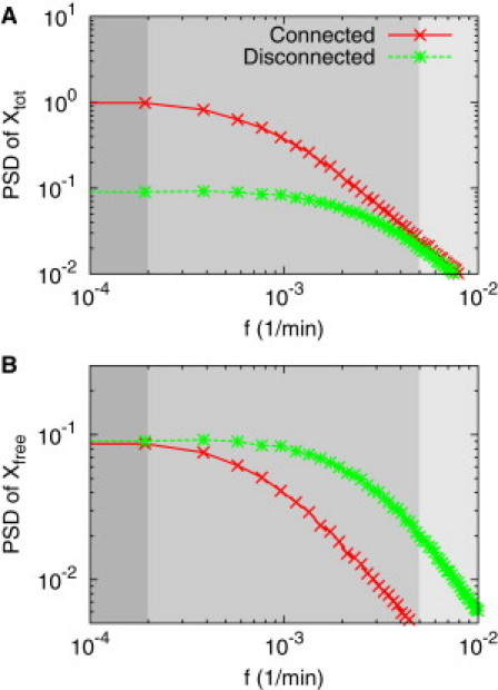
Power spectral densities of signal X_tot and X_free shown in Fig. 5A: The power spectral densities (one-sided) are obtained from the autocorrelation functions of X_tot and X_free. The low frequency components of signal X_free are not affected by the connection to a downstream component (B), whereasthe high-frequency components of X_tot are not (A). The threshold point, where the PSD starts to drop, is shifted to the left for both X_free and X_tot, due to the connection. Three regions of frequency colored above correspond, respectively, from left to right, to the low-frequency region where the signal X_free is not affected, whereas X_tot is an intermediate region where both X_free and X_tot are affected, and a high-frequency region where X_tot is not affected whereas X_free is.

Modularity in circuit dynamics and two choices of output signals: X_free or X_tot?

Fig. 6 shows some very interesting aspects of the frequency response in the circuit. The noise spectrum of signal X_tot (the total number of the transcription factor) changes significantly at low enough frequencies whereas it does not at high enough frequency, but that of signal X_free (the number of the unbound transcription factor) shows the opposite behavior. This implies that the signal X_free is not affected by the downstream regulation when the circuit is operated at low frequency, and the signal X_tot does not when operated at high frequency, although the retroactivity is still causing a significant change in the frequency bandwidth. Thus, we propose that circuit dynamics can be investigated in a modular way by choosing an appropriate output signal, either X_free or X_tot, depending on the magnitude of the operating frequency.

To validate the above prediction, we simulate the MIP described by Fig. 2 B deterministically, with α allowed to oscillate at different frequencies, which are chosen from three different regions indicated in Fig. 6:

$$\alpha \left(t\right)=1+0.1\sin \left(2\pi ft\right)$$ (12)

with $f=0.001/2\pi$, $0.01/2\pi$, and $0.05/2\pi$ min⁻¹ (see Fig. 7). Output signals X_free and X_tot show oscillations with basal levels:

$$X_{free}\left(t\right)={\overline{X}}_{free}+\delta X_{free}\left(t\right)$$

or

$$X_{tot}\left(t\right)={\overline{X}}_{tot}+\delta X_{tot}\left(t\right).$$

We compare the oscillatory components (δX_free and δX_tot) of the output signals for the two different cases when the output is connected and disconnected (Fig. 7). At the low frequency f = 0.001/2π min⁻¹, δX_free does not change due to the downstream regulation whereas δX_tot does. At high frequency f = 0.05/2π min⁻¹, δX_free changes due to the regulation whereas δX_tot does not. At the intermediate frequency f = 0.01/2π min⁻¹, both the signals X_free and X_tot change. This verifies the prediction based on power spectral densities, and implies that the modularity of gene circuits can be tested by observing gene expression noise.

Figure 7.

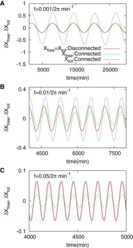
Signals X_free and X_tot in the module interface process shown in Fig. 2B: These two signals are compared for different values of frequency when deterministically simulated. The translation rate α is given as a time-varying signal with a harmonic oscillation as shown in Eq. 12. The signal X_free and X_tot show distinct behaviors for different frequencies corresponding to the three colored regions shown in Fig. 6. The parameter values are identical to those used in Fig. 5A.

Example: dimer transcription factor with negative feedback

In this example, we consider a MIP involving dimer transcription factors that are under inhibitory self-regulation. The MIP can be modeled using the following set of reactions:

$$\begin{array}{l}\stackrel{\frac{\alpha }{1+\beta X_2}}{\to }X\stackrel{\gamma X}{\to }ø\hfill \\ X+X\underset{k_2{X}_2}{\overset{k_{1}X\left(X-1\right)}{\rightleftharpoons }}{X}_2\stackrel{{\gamma }_2{X}_2}{\to }ø\hfill \\ X_2+P_f\underset{k_{off}{P}_b}{\overset{k_{on}{X}_2{P}_f}{\rightleftharpoons }}{P}_b,\hfill \end{array}$$

where a parameter β controls the strength of the negative feedback. For the case without feedback (β = 0), we used α = 20 (nM/h), γ = 2(1/h), k₁ = 20 (1/nM/h), k₂ = 1 (1/h), γ₂ = 2 (1/h), k_on = 10 (1/nM/h), and k_off = 10 (1/h). For the case with negative feedback β = 0.25, we used α = 43(nM/h) to adjust the level of X to the one without any feedback. Here the volume of the host cell is assumed to be 1 μm³, and thus the unit of nM is interchanged with that of a copy number.

We performed simulations by using Gillespie's stochastic simulation algorithm (35). The values of concentrations were recorded 50 times/h for 48 h (corresponding to experimental time). The autocorrelation function of the total TF concentration (X + 2X₂ + 2P_b) was computed for the recorded series, and was fitted to an exponential function by using a linear fit in a semilog scale (log scale in y axis and normal scale in x axis). The fitted slope estimates the inverse of correlation time of the stochastic fluctuations in the total TF concentration. The error bar of the correlation time was estimated from 10 independent replicates of the autocorrelation function. Retroactivity was computed by using Eq. 10.

Fig. 8 B shows the match between the deterministic and stochastic retroactivities. However, if the autocorrelation function of X or X₂ has been used, the match would not hold well due to the sudden decrease in the autocorrelation as shown in Fig. 8 A (a careful choice of a linear region is required for estimating the correlation time). The decrease is due to the fast decorrelation effect of dimerization, dimer dissociation, and dimer binding-unbinding reactions. This is why we have used the total number of TFs for estimating retroactivity (refer to the Discussion for more detail). Here the deterministic retroactivity was obtained by using Mathematica (Wolfram Research, Champaign, IL) (36) (a notebook file is provided as the Supporting Material) as the mathematical equation for retroactivity is quite complicating compared with the simple monomer case without any feedback. Fig. 8 B also shows the negative feedback decreases retroactivity as proposed by Del Vecchio et al. (8)

Figure 8.

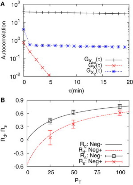
Module interface process involving dimer TFs that are under negative feedback. (A) The autocorrelations of free TF monomer units (X) and dimer TFs (X₂) quickly decrease for small τ ≲ 2 min due to the effect of dimerization, dimer dissociation, and dimer binding-unbinding reactions, whereas that of the total number of the TFs (monomer units) does not. The plot is for the case with negative feedback. Similar behavior was observed for the case without feedback (graph not shown). (B) Stochastic retroactivity matches the deterministic one and the negative feedback decreases the value of the retroactivity. The retroactivity is defined as the relative decrease in the cutoff frequency with respect to the isolated case without any feedback: $R\equiv \left({\tau }_{P_T}-{\tau }_0^{Neg-}\right)/{\tau }_{P_T}$. Refer to Example: Dimer Transcription Factor with Negative Feedback in text for parameter values.

Computational approach for estimating retroactivity from gene expression noise

In this subsection, we show how to measure retroactivity based on fluorescence data from single cell experiments. Synthetic circuits are often transfected into host cells, e.g., E. coli, which duplicate themselves by completing cell cycles. This causes the intracellular concentrations to fluctuate. In addition, the host cells are under other unidentified extrinsic noise sources. Such extrinsic noise has been shown to affect the autocorrelation functions (13–16) and needs to be taken into account for estimating the level of modularity.

When the lifetime of a TF is longer than the correlation time of the extrinsic noise (which is typically in the order of magnitude of cell doubling time (13–16)), the apparent lifetime of the TF will be dominantly determined by the cell doubling time. Then, the effect of retroactivity becomes negligible if we assume that the cell doubling time is not affected by the downstream module connection. Thus, to observe the retroactive effect, it is important to reduce the actual lifetime below the cell doubling time. This can be achieved, for example, by inserting carboxy-terminal tags that are recognized by proteases in E. coli (27,37).

When such a degradation-tagged transcription factor has a fluorescence marker, the autocorrelation function of the fluorescence emitted from the TF can be fitted to the function (see the Materials and Methods)

$$G_{X_{tot}}\left(\tau \right)=A{e}^{-{\gamma }_E\tau }+B{e}^{-\left({\gamma }_E+1/T\right)\tau },$$ (13)

with γ_E = log(2)/T_d and T the correlation time. The above form of the autocorrelation has been investigated in its Fourier transform (power spectral density) by Austin et al. (14) by using a plasmid containing a GFP variant with its half-life reduced. They did not consider the retroactivity dependence in the correlation time. The power spectral density, a Fourier transform of the autocorrelation function Eq. 13, is obtained as (14)

$$\tilde{G}\left(\omega \right)=\frac{2A{\gamma }_E}{{\gamma }_E^2+{\omega }^2}+\frac{2B\left({\gamma }_E+1/T\right)}{{\left({\gamma }_E+1/T\right)}^2+{\omega }^2}.$$

Depending on the relative magnitude of A and B, the bandwidth is determined by either γ_E and γ_E + 1/T or both.

We propose the following data analysis procedures, to estimate retroactivity:

• 1.Obtain single cell fluorescence trajectories by connecting each trajectory belonging to a cell lineage, by following the method described in Austin et al. (14).
• 2.Estimate the autocorrelation function of the fluorescence.
• 3.Perform a nonlinear fit by using Eq. 13 to estimate γ_E and T. Alternatively, estimate γ_E = log(2)/T_d by measuring cell doubling time (T_d) from the cell lineage, and then perform a nonlinear fit to estimate T by using Eq. 13.
• 4.Estimate the retroactivity: Repeat the above procedures to estimate the correlation times for the isolated and connected cases, respectively, and compute retroactivity by using Eq. 10.

We present a model for gene expression in the Materials and Methods, where we derive the above autocorrelation function equation, Eq. 13. We show that this equation is consistent with the ones used in current in vivo experiments (13–16). The model process is described in the Langevin dynamics framework, with the retroactive effect taken into account.

Discussion

We have proposed a numerical estimation method for retroactivity based on gene expression noise. The retroactivity quantifies the slowdown of kinetics of an upstream module output. To observe this dynamical effect, we have investigated gene expression noise that is caused by continuous perturbations from intrinsic and extrinsic sources that exist naturally in the system, without resorting to the manipulation of external perturbations.

We have shown that the correlation time of the output noise increases when the output is allowed to regulate a downstream module. This corresponds to a decrease in the bandwidth of the power spectral density (34) and reflects the fact that the module interface process filters out the high-frequency signal components of X_tot more strongly.

We have shown that the signals X_free and X_tot reveal different power spectral densities. The origin of this different behavior is as follows. Consider the case where the circuit operates in the low-frequency region. The mean level of X_free, corresponding to the zero frequency component, is determined by its synthesis and degradation rate because binding and unbinding reactions are balanced (〈X_free〉 = α/γ). The same argument is applied for the low frequency region (ω) colored in dark gray in Fig. 6, where the balance still holds, and the two PSD of X_free when connected and disconnected are almost the same as each other. This means that the low-frequency components of signal X_free are not distorted by the downstream module regulation. Therefore, when the dynamics of the individual modules are described by X_free, the signal distortion in X_free due to the retroactivity can be minimized by operating at the low frequency.

In the case that the circuit operates in the high frequency region, we choose the signal X_tot rather than X_free to minimize the retroactive effect because the two PSDs of X_tot when connected and disconnected match each other at the high frequencies as shown in Fig. 6. Mathematically, both the PSDs of X_tot converge to W_I/2πω² as ω ≫ 1/T by using Eq. 11. We note that the PSD of X_tot at the low frequencies changes due to the downstream module regulation because there is an extra amount of bound TFs. This PSD study implies that a modular description is possible by choosing the right signal variables either X_free or X_tot depending on the operating frequencies.

In the estimation of correlation times, we have used the signal X_tot rather than X_free. There are two reasons for this. The first is that the total number can be experimentally observable when the output TF is tagged for fluorescence under the assumption that the fluorescence intensity does not change when the TFs are bound.

The second is that it directly reflects the dynamics of the timescale of interest (of the order of cell-doubling time or less) resulting in more accurate estimates of correlation times when compared with the case that X_free is used; as shown in Fig. 5 A, the autocorrelation of X_free shows a sudden drop for small values of τ and this drop requires a careful choice of the linear region to obtain the response time. When the binding-unbinding reactions are slow, the region of the sudden initial drop is expanded and a more careful analysis would be required (graph not shown). However, the autocorrelation of X_tot does not show any initial sudden drop at all, since all the fluctuations originating from the binding-unbinding reactions do not cause any effect on X_tot (here we did not assume any quasi-steady-state approximation, but chose a different variable that does not fluctuate due to the binding-unbinding reactions). Thus, the variable X_tot can be considered a pure slow mode (8,38), and this is why we have used the autocorrelation of X_tot.

To measure the correlation time, we have fitted the autocorrelation to a pure exponential function (when extrinsic noise is not considered). In most of the cases appropriate for experiments, the fitting was accurate within the time interval (τ) of our interest. However, in some cases (the circled ones in Fig. 5 B) it was not (one example is shown in Fig. 9). Such nonpure exponential autocorrelation would appear in general if you were able to reach a larger value of τ. This is due to the fact that the degradation rate function of X_tot is highly nonlinear in X_tot (see Fig. 3, B and C): The response time, defined as the inverse of the slope of degradation rate function, can be highly dependent on the magnitude and sign (above or below the mean) of the fluctuations (with respect to the mean) significantly. If the fluctuations are negative/positive and its magnitude is sufficiently large, the slope can decrease/increase significantly, i.e., both the response time and the correlation time can increase/decrease significantly. This implies that the autocorrelations become the sum of many exponentials having different response time constants (correlation times). The fluctuations having a long response time can persist in its correlation for the long time interval, contributing dominantly to an autocorrelation function for the region of large τ. Therefore, it is typical in retroactive systems (whose degradation of X_tot is highly nonlinear) to show that the slope of the autocorrelation (in the semilog plot) decreases for large values of τ (e.g., τ ≳ 25 min in Fig. 9). This was, however, not apparent in most cases that were experimentally reasonable within the time interval of interest.

Figure 9.

Nonexponential autocorrelation function for the module interface process shown in Fig. 2B: The case that $G_{X_{tot}}\left(\tau \right)$ is not a pure exponential function is considered (one of the circled cases in Fig. 5: K_d = 0.001 nM, 〈X〉 = α/γ = 0.1 nM, and P_T = 100 nM). For small τ, the slope of $\log G_{X_{tot}}$ converges to the value computed in the deterministic case, i.e., −γ(1 − R_d), whereas it decreases for larger τ. The response time was obtained in the linear region between τ = 0 and 20 min. Parameters: α = 0.1 nM h⁻¹, γ = 1 h⁻¹, k_on = 10 nM⁻¹ h⁻¹, and k_off = 0.01 h⁻¹.

In summary, we have considered a module interface process in a genetic circuit and have shown that the noise correlation time increases after the output of the circuit module is connected to another module. We call such changes in the correlation time “stochastic retroactivity”. We have proposed an experimental estimation method for measuring the retroactivity based on gene expression noise. We have also proposed that, depending on the magnitude of an operating frequency, the circuit dynamics can be analyzed in a modular fashion by choosing an appropriate circuit output signal. This study, based on gene expression noise, can serve as an important method for characterizing interface conditions between two synthetic modules and eventually provide a step toward large-scale circuit design for synthetic biology.

References

- 1.Purnick P.E.M., Weiss R. The second wave of synthetic biology: from modules to systems. Nat. Rev. Mol. Cell Biol. 2009;10:410–422. doi: 10.1038/nrm2698. [DOI] [PubMed] [Google Scholar]
- 2.Keasling J.D. Synthetic biology for synthetic chemistry. ACS Chem. Biol. 2008;3:64–76. doi: 10.1021/cb7002434. [DOI] [PubMed] [Google Scholar]
- 3.Voigt C.A. Genetic parts to program bacteria. Curr. Opin. Biotechnol. 2006;17:548–557. doi: 10.1016/j.copbio.2006.09.001. [DOI] [PubMed] [Google Scholar]
- 4.Sprinzak D., Elowitz M.B. Reconstruction of genetic circuits. Nature. 2005;438:443–448. doi: 10.1038/nature04335. [DOI] [PubMed] [Google Scholar]
- 5.Endy D. Foundations for engineering biology. Nature. 2005;438:449–453. doi: 10.1038/nature04342. [DOI] [PubMed] [Google Scholar]
- 6.Canton B., Labno A., Endy D. Refinement and standardization of synthetic biological parts and devices. Nat. Biotechnol. 2008;26:787–793. doi: 10.1038/nbt1413. [DOI] [PubMed] [Google Scholar]
- 7.Chandran D., Bergmann F.T., Sauro H.M. TinkerCell: Modular CAD Tool for Synthetic Biology. J. Biol. Eng. 2009;4:3–19. doi: 10.1186/1754-1611-3-19. [DOI] [PMC free article] [PubMed] [Google Scholar]
- 8.Del Vecchio D., Ninfa A.J., Sontag E.D. Modular cell biology: retroactivity and insulation. Mol. Syst. Biol. 2008;4:161. doi: 10.1038/msb4100204. [DOI] [PMC free article] [PubMed] [Google Scholar]
- 9.Arkin A., Ross J., McAdams H.H. Stochastic kinetic analysis of developmental pathway bifurcation in phage λ-infected Escherichia coli cells. Genetics. 1998;149:1633–1648. doi: 10.1093/genetics/149.4.1633. [DOI] [PMC free article] [PubMed] [Google Scholar]
- 10.Elowitz M.B., Levine A.J., Swain P.S. Stochastic gene expression in a single cell. Science. 2002;297:1183–1186. doi: 10.1126/science.1070919. [DOI] [PubMed] [Google Scholar]
- 11.Ozbudak E.M., Thattai M., van Oudenaarden A. Regulation of noise in the expression of a single gene. Nat. Genet. 2002;31:69–73. doi: 10.1038/ng869. [DOI] [PubMed] [Google Scholar]
- 12.Elf J., Li G.-W., Xie X.S. Probing transcription factor dynamics at the single-molecule level in a living cell. Science. 2007;316:1191–1194. doi: 10.1126/science.1141967. [DOI] [PMC free article] [PubMed] [Google Scholar]
- 13.Rosenfeld N., Young J.W., Elowitz M.B. Gene regulation at the single-cell level. Science. 2005;307:1962–1965. doi: 10.1126/science.1106914. [DOI] [PubMed] [Google Scholar]
- 14.Austin D.W., Allen M.S., Simpson M.L. Gene network shaping of inherent noise spectra. Nature. 2006;439:608–611. doi: 10.1038/nature04194. [DOI] [PubMed] [Google Scholar]
- 15.Weinberger L.S., Dar R.D., Simpson M.L. Transient-mediated fate determination in a transcriptional circuit of HIV. Nat. Genet. 2008;40:466–470. doi: 10.1038/ng.116. [DOI] [PubMed] [Google Scholar]
- 16.Dunlop M.J., Cox R.S., 3rd, Elowitz M.B. Regulatory activity revealed by dynamic correlations in gene expression noise. Nat. Genet. 2008;40:1493–1498. doi: 10.1038/ng.281. [DOI] [PMC free article] [PubMed] [Google Scholar]
- 17.Rao C.V., Wolf D.M., Arkin A.P. Control, exploitation and tolerance of intracellular noise. Nature. 2002;420:231–237. doi: 10.1038/nature01258. [DOI] [PubMed] [Google Scholar]
- 18.Raser J.M., O'Shea E.K. Control of stochasticity in eukaryotic gene expression. Science. 2004;304:1811–1814. doi: 10.1126/science.1098641. [DOI] [PMC free article] [PubMed] [Google Scholar]
- 19.Kaern M., Elston T.C., Collins J.J. Stochasticity in gene expression: from theories to phenotypes. Nat. Rev. Genet. 2005;6:451–464. doi: 10.1038/nrg1615. [DOI] [PubMed] [Google Scholar]
- 20.Shahrezaei V., Ollivier J.F., Swain P.S. Colored extrinsic fluctuations and stochastic gene expression. Mol. Syst. Biol. 2008;4:196. doi: 10.1038/msb.2008.31. [DOI] [PMC free article] [PubMed] [Google Scholar]
- 21.Munsky B., Trinh B., Khammash M. Listening to the noise: random fluctuations reveal gene network parameters. Mol. Syst. Biol. 2009;5:318. doi: 10.1038/msb.2009.75. [DOI] [PMC free article] [PubMed] [Google Scholar]
- 22.Anishchenko V.S., Astakhov V., Schimansky-Geier L. Springer-Verlag; Berlin, Germany: 2002. Nonlinear Dynamics of Chaotic and Stochastic Systems. [Google Scholar]
- 23.Kepler T.B., Elston T.C. Stochasticity in transcriptional regulation: origins, consequences, and mathematical representations. Biophys. J. 2001;81:3116–3136. doi: 10.1016/S0006-3495(01)75949-8. [DOI] [PMC free article] [PubMed] [Google Scholar]
- 24.Simpson M.L., Cox C.D., Sayler G.S. Frequency domain chemical Langevin analysis of stochasticity in gene transcriptional regulation. J. Theor. Biol. 2004;229:383–394. doi: 10.1016/j.jtbi.2004.04.017. [DOI] [PubMed] [Google Scholar]
- 25.Sauro H.M., Hucka M., Kitano H. Next generation simulation tools: the Systems Biology Workbench and BioSPICE integration. OMICS. 2003;7:355–372. doi: 10.1089/153623103322637670. [DOI] [PubMed] [Google Scholar]
- 26.Bergmann, F., and H. Sauro. 2006. SBW—a modular framework for systems biology. In Proceedings of the 38th Conference on Winter Simulation. Winter Simulation Conference, 1637–1645.
- 27.Elowitz M.B., Leibler S. A synthetic oscillatory network of transcriptional regulators. Nature. 2000;403:335–338. doi: 10.1038/35002125. [DOI] [PubMed] [Google Scholar]
- 28.Buchler N.E., Cross F.R. Protein sequestration generates a flexible ultrasensitive response in a genetic network. Mol. Syst. Biol. 2009;5:272. doi: 10.1038/msb.2009.30. [DOI] [PMC free article] [PubMed] [Google Scholar]
- 29.Scholz O., Schubert P., Hillen W. Tet repressor induction without Mg2+ Biochemistry. 2000;39:10914–10920. doi: 10.1021/bi001018p. [DOI] [PubMed] [Google Scholar]
- 30.Setty Y., Mayo A.E., Alon U. Detailed map of a cis-regulatory input function. Proc. Natl. Acad. Sci. USA. 2003;100:7702–7707. doi: 10.1073/pnas.1230759100. [DOI] [PMC free article] [PubMed] [Google Scholar]
- 31.Pompeani A.J., Irgon J.J., Bassler B.L. The Vibrio harveyi master quorum-sensing regulator, LuxR, a TetR-type protein is both an activator and a repressor: DNA recognition and binding specificity at target promoters. Mol. Microbiol. 2008;70:76–88. doi: 10.1111/j.1365-2958.2008.06389.x. [DOI] [PMC free article] [PubMed] [Google Scholar]
- 32.Nilsson J., Riedel S. Pearson/Prentice Hall; Upper Saddle River, NJ: 2008. Electric Circuits. [Google Scholar]
- 33.Simpson M.L., Cox C.D., Sayler G.S. Frequency domain analysis of noise in autoregulated gene circuits. Proc. Natl. Acad. Sci. USA. 2003;100:4551–4556. doi: 10.1073/pnas.0736140100. [DOI] [PMC free article] [PubMed] [Google Scholar]
- 34.Jayanthi, S., and D. Del Vecchio. 2009. On the compromise between retroactivity attenuation and noise amplification in gene regulatory networks. Proc. IEEE Conf. Dec. Control. 15–18 December 2009; Shanghai, China, 2010. 4565–4571.
- 35.Gillespie D.T. Exact stochastic simulation of coupled chemical reactions. J. Phys. Chem. 1977;81:2340–2361. [Google Scholar]
- 36.Wolfram S. Advanced Book Program, Addison-Wesley; Redwood City, CA: 1988. Mathematica: a System for Doing Mathematics by Computer. [Google Scholar]
- 37.Herman C., Thévenet D., D'Ari R. Degradation of carboxy-terminal-tagged cytoplasmic proteins by the Escherichia coli protease HflB (FtsH) Genes Dev. 1998;12:1348–1355. doi: 10.1101/gad.12.9.1348. [DOI] [PMC free article] [PubMed] [Google Scholar]
- 38.Rao C.V., Arkin A.P. Stochastic chemical kinetics and the quasi-steady-state assumption: application to the Gillespie algorithm. J. Chem. Phys. 2003;118:4999–5010. [Google Scholar]
Associated Data
This section collects any data citations, data availability statements, or supplementary materials included in this article.