Computer-aided Prostate Cancer Detection using Texture Features and Clinical Features in Ultrasound Image

Abstract

In this paper, we propose a new prostate detection method using multiresolution autocorrelation texture features and clinical features such as location and shape of tumor. With the proposed method, we can detect cancerous tissues efficiently with high specificity (about 90–95%)and high sensitivity (about 92–96%) by the measurement of the number of correctly classified pixels. Multiresolution autocorrelation can detect cancerous tissues efficiently, and clinical knowledge helps to discriminate the cancer region by location and shape of the region and increases specificity. The support vector machine is used to classify tissues based on those features. The proposed method will be helpful in formulating a more reliable diagnosis, increasing diagnosis efficiency.

Introduction

Prostate cancer is the second most commonly diagnosed cancer in elderly men. Because life expectancy is increasing, early detection and intervention of prostate cancer is extremely important to reduce the associated death rate. Different types of diagnostics, such as digital rectal examination (DRE) and prostate-specific antigen (PSA), are used today to detect prostate cancer at an early stage. Those two methods are used as a combination to make a reliable diagnosis. However, DRE easily misses small tumors, and PSA values are dependent on several factors that are not caused only by prostate cancer.⁶ Several imaging types can be used to make a more reliable diagnosis, and transrectal ultrasound (TRUS) is one of them.

The use of the TRUS test has become widespread because of its ability to visualize the prostate gland with no injurious effects and at inexpensive cost as well as its real-time characteristic. While the TRUS test is currently the most widely used imaging method, it has relatively low predictive value in detecting cancer¹ because of considerable overlap of benign and malignant lesion characteristics, in addition to the fact that its predictive ability is highly dependent on the radiologist’s interpretation. To improve the current TRUS test, a real-time computer-aided diagnosis system with high performance is required. It is because the general process of TRUS works in real time, unlike other imaging modalities such as computed tomography or magnetic resonance imaging. The TRUS test system must give some useful information in real time to the radiologist. Unfortunately, no TRUS computer-aided diagnosis system for prostate cancer detection exists till now.

As an effort to invent a practical computer-aided system for the TRUS test, an automatic process of finding cancer in a TRUS image has been suggested in this paper. This can help radiologists by suggesting the search region in an ultrasound image. The automated process can save time routinely spent for visual inspection of the TRUS image by radiologists and increase diagnosis efficiency. Therefore, the suggested method shows prospective directions for the system available in real world.

In spite of the importance of early detection of prostate cancer, only a few works have been published on computer-aided diagnosis of prostate cancer. In a research introduced by Ellis et al.,¹³ the authors report that the TRUS test, using the features of maximum height, width, volume, and so on of prostate, showed 64% accuracy in classifying benign and malignant lesions. In spite that their research does not show the outstanding results, it is meaningful for they correlated the pathological examination with TRUS image features. In the TRUS examination described by Huynen et al.,² texture features of co-occurrence matrices, which were introduced by Haralick et al.,⁵ were used to classify benign and cancerous tissue. Good results were reported with this method (80% sensitivity and 88% specificity). With a similar approach, de la Rosette et al.³ tested the capacity of the automated urologic diagnosis expert system to detect cancer. Values of 90% sensitivity and 64% specificity were obtained. Llobet et al.⁶ also used co-occurrence matrices, known as the gray level dependence matrix, for texture features. They applied two classifiers, k-nearest neighborhood and Hidden Markov models, to classify the pixels and they compared both results. Their research showed 57.2% sensitivity and 61.0% specificity when the threshold they used was tuned to get an appropriate balance, while 93.6% sensitivity and 14.8% specificity in a maximum sensitivity case. Other texture features such as autocorrelation, frequency, energy, and discontinuity were used to discriminate between benign and cancerous tissue by Yfantis et al.⁴ However, the author did not mention the sensitivity or specificity of those features in their study.⁴

The existing papers mainly used texture features. However, discrimination between benign and cancerous tissues based only on texture features is extremely difficult due to the problem of imperfect supervision (incorrect labeling of specific pixels).⁶ Pixels cannot be labeled as positive or negative by simply analyzing the images at the texture level. Therefore, it is necessary to analyze other features of cancerous regions as well as discriminative texture features.

In this paper, we propose new multiresolution autocorrelation texture features and clinical features such as location and shape of tumor for prostate cancer detection. Multiresolution autocorrelation can detect cancerous tissues efficiently with high specificity and sensitivity. Clinical features help to discriminate the cancer region by location and the shape of the region, and they increase specificity of cancer detection. The proposed method can help urologists to analyze the prostate TRUS images efficiently, limiting the search area to the detected cancerous region. It also shows high specificity together with maintaining high sensitivity. Therefore, the detected region can help urologists to reduce the analysis variance among them. Our method aims to find the location of the cancer region in the ultrasound image, searching from the top left to bottom right of the TRUS image. The location of the cancerous region, as well as cancer detection performance itself, is important. The suggested method shows prospective results for the automated diagnosis; however, further research is required to accelerate the speed of this method for availability in real-time scanning.

Cancer Detection Method

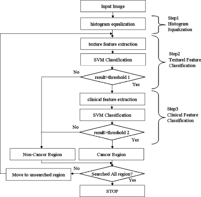
A large portion of the ultrasound image of the prostate gland is a nonprostate lesion. To decrease the search area of the image, the darker region is segmented by histogram equalization. Since the prostate region is relatively darker than the surrounding region, the segmented region is considered to be a prostate lesion. After initial prostate segmentation, multiresolution autocorrelation is extracted to be used as a feature. If this autocorrelation is extracted from the cancerous region, it is considered to be a feature of the cancer region. If it is extracted from the noncancer region, then it is considered to be a feature of the noncancer region. These features become training data for the support vector machine (SVM). After training is finished, the sliding window from top left to bottom right of the image is tested by the trained SVM. If it is considered as cancer, the center pixel of the window patch is considered to be a cancer pixel. This process is repeated until the whole image is tested. Figure 1 shows the overall procedure of the proposed method.

Fig. 1.

Overall procedure of proposed method.

Histogram Equalization

Histogram equalization increases the brightness difference between hypoechoic tissue (dark region) and hyperechoic tissue (bright region). Since prostate is darker than the surrounding lesion, histogram equalization makes prostate much darker than its surrounding. After histogram equalization, we make a binary image to limit the searching area only to the darker region. Each pixel value in the TRUS image is transformed by the equation defined by

where S_k is transformed value of intensity value r_k, T is the transforming function, P_k is the probability, n_j is the number of pixels with intensity value r_j, and n is the number of all pixels. After histogram equalization is done, the darker region is segmented to be the searching area. The accuracy of the initial segmentation by histogram equalization was about 75%, measured by the accordance with the boundary of prostate. However, it included about 98% of the cancerous lesions that were pointed by a radiologist. If a method to detect the precise prostate boundary is used, it will show better performance. Figure 2 shows the result of histogram equalization, and Figure 3 shows the segmented binary image. In this research, texture features are extracted in the segmented region.

Fig. 2.

Original image (left) and transformed image (right).

Fig. 3.

Segmented binary image.

Then, only the image window in the prostate tissue becomes the region of interest (ROI).

Texture Feature Extraction

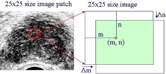
Different tissues have markedly different textures. Therefore, texture descriptors of the window image can be good features of cancerous tissue. In this research, the brightness of the tissue is used as a texture feature.⁷ In addition to brightness, multiresolution autocorrelation coeffcients in two dimensions are used. Figure 4 shows the concept of autocorrelation, and its coefficients have shapes like in Figure 5.

Fig. 4.

Autocorrelation coefficients extraction.

Fig. 5.

Graph of the extracted autocorrelation coefficients.

Autocorrelation coefficients are defined as,⁸

where

where m and n are the x- and y-coordinate values of the center point, f(x, y) is the pixel values of the window image, and is the mean of f(x, y). How to choose the size of the image window and parameters of Δm and Δn are dependent on the problems. The following matrix is the extracted texture feature.

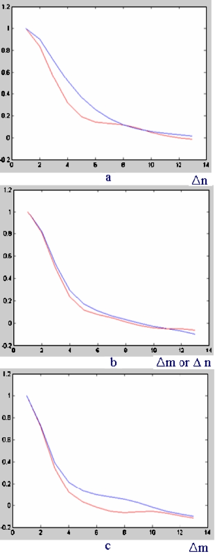
Different textures show different shapes of autocorrelation coefficients. The three-dimensional shape of autocorrelation is projected into two dimensions according to specific direction so that the difference of shape between cancerous tissue and benign (noncancer) tissue can be noticed clearly in Figure 6.

Fig. 6.

a 0° direction, b 45° direction, c 90° direction.

The red line represents the autocorrelation shape of cancerous tissue, and the blue line represents the autocorrelation shape of noncancer tissue. In spite that it is difficult to discriminate between the two line shapes in Figure 6a, Figure 6b and c show that autocorrelation shift Δm, Δn = 7–9 may maximize the accumulated difference between cancer tissue and noncancer tissue while balancing computational burden and discriminative ability. To extract multiresolution autocorrelation of texture, autocorrelation coefficients of 12 times down-sampled image, as well as those of the original size image, must be extracted. In this study, the radius of Δm = Δn = 7 (7 × 7 = 49 coefficients) with a 25 × 25 size image window for the original image, and in the same way, the radius of Δm = Δn = 5 (5 × 5 = 25 coefficients) with a 15 × 15 size image window for 1/2 times down-sampled image were used. Figure 7 shows how to extract the feature vector of multiresolution autocorrelation coefficients.

Fig. 7.

Feature extraction of multiresolution autocorrelation coefficients.

The choice on the values of Δm, Δn was made considering the experimental results that the best performance was achieved when Δm, Δn = 7 for the original size image. The other values of Δm, Δn caused the decrease in specificity or sensitivity. Table 1 shows the influence of Δm, Δn on the performance. The result of Table 1 was gained by the experiment on the original size image. As can be seen, the performance at Δm, Δn = 7 achieves the best result in the original size image. In the similar way, Δm, Δn = 5 achieves the best result in the down-sampled image in our database. In this research, those two selections of Δm, Δn = 7 in the original size image and Δm, Δn = 5 in the 1/2 times down-sampled image are combined to be used as texture features.

Table 1.

The Influence of Δm, Δn on Performance

Δm, Δn	Sensitivity	Specificity
15	79.6	87.8
11	81.5	85.5
9	83.5	86.3
7	87.3	85.1
5	84.1	85.1

The extracted autocorrelation features can be training data for SVM as well as test data for the trained SVM. The incremental use of the autocorrelation coefficients from the down-sampled image enables the texture features to have more information about the lesion. Originally, the autocorrelation coefficients have the information on the self-similarity of the image window. Therefore, the additional usage of the coefficients from the down-sampled image gives the information of self-similarity in the down-sampled image. The difference between the multiresolution autocorrelation and the large-shift single resolution autocorrelation is that the large-shift autocorrelation can be easily influenced by small noise and resolution variance, while the multiresolution autocorrelation has more robustness to small noise and resolution variance, as well as much less computation time. If the tested image window is classified to be cancerous, its center pixel is labeled to be a cancer pixel.

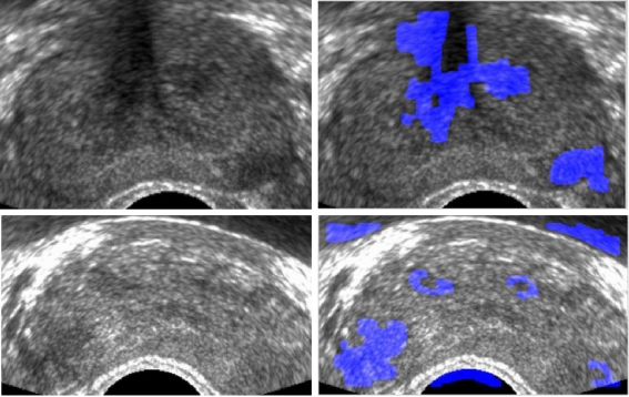
In Figure 8, cancer pixel classification results are shown. The cancer pixels are colored blue. However, they still have a lot of false-positive cancer regions. To reduce the false-positive rate (FPR), more information about the cancer tissue must be taken into account.

Fig. 8.

Cancer detection results by texture feature: original images (left) and cancer-detected images (right).

Clinical Feature Extraction

Texture features can be good discriminative features of cancer tissue and noncancer tissue. However, as Figure 8 shows, mere texture features are not enough for cancer detection. Therefore, clinical knowledge-based features such as the location of the cancerous region and the shape of the cancerous region are applied in this research.

Location Feature Clinically, the peripheral zone (the lower part of the TRUS prostate image) is the most frequent site of prostate cancer, and around 70% of prostate cancers originate from the peripheral zone.⁹ Therefore, the hypoechoic region (dark region) with cancer texture in the peripheral zone has a high possibility of cancer, while the hypoechoic region with the cancer texture in the other zone of prostate (upper part of the TRUS image) has a low possibility of cancer (Fig. 9).

Fig. 9.

Cancer possibility of the prostate gland by location.

Shape Feature The hypoechoic region of an ellipse shape has a higher possibility of cancer, while that of an irregular shape has a lower possibility of cancer.¹⁰ To estimate the cancer-textured region as an ellipse, the difference between the ellipse and the boundary of the cancerous region is integrated. If the cancerous region has a similar shape as an ellipse, the integration will be small. The longest axis and its orthogonal axis of cancerous region boundary become the estimation of radial axes of an ellipse. Then, the coordinate of the boundary of the cancerous region and the estimated ellipse is transformed to a polar coordinate. After coordinate transformation, the difference over the ellipse and the boundary is integrated. Figure 10 shows the cancerous region boundary and the estimated ellipse. The difference between the ellipse and the boundary of the cancerous region is defined as

where r₁ is the distance from the center of the ellipse to the boundary contour of ellipse, r₂ is the distance from the center of the ellipse to the boundary contour of the cancer region, and θ is the angle between r₁ and the horizontal axis. Thus, the clinical feature is composed of location and shape features. To get appropriate clinical features of cancer, true locations of cancer regions are provided by a radiologist. Then, the clinical features of the true cancer regions become positive training data for the cancer region, and the clinical features of the other region become negative training data. To get the training database for the clinical features, 310 contours from the whole database (51 images) were gained first. Then 150 contours were randomly selected from those 310 contours to extract the clinical features of training data. Among those 150 contours, 80 contours of the true cancer region become the data for true cancer features, and the remained 70 contours become the data for noncancer features. The location and shape features are trained using SVM. The trained SVM can predict whether a specific region belongs to the cancer or benign tissue.

Fig. 10.

Cancer boundary and estimated ellipse (left) and shape difference (right).

In Figure 11, the green and red region is predicted as a cancer region by trained SVM. The red region is considered as a cancer region by the radiologist. The green region is considered as a false-positive region. The blue region has cancer texture but is considered a noncancer region by clinical features.

Fig. 11.

Original images (left) and cancer detected images (right).

Classification by Support Vector Machine

In the proposed method, SVM^{11, 12} was used as the classifier. SVM has an advantage over traditional neural networks in generalization performance. While neural networks such as multiple layer perceptron perform at a low error rate on test data, SVM performs excellent generalization, which is called structural risk minimization. The purpose of structural risk minimization is to set an upper bound on the expected generalization error. While there exist numerous decision planes that show the zero error rate on the training set, the performance of the decision planes on test data will vary. Among those decision planes, the decision plane with the maximum margin between two classes will achieve optimal worst-case generalization performance. While SVM was originally designed to solve problems where data can be separated by a linear decision boundary, it can still deal with problems that are not linearly separable by using kernel functions such as Gaussian functions, polynomial functions, and sigmoid functions. In this paper, the Gaussian kernel function was chosen with the input vector composed of the texture and clinical features. The classification result of SVM was used to distinguish between the cancer region and noncancer region in the ultrasound image.

Experiments

Classifications by support vector classification experiments were carried out to test the performance of the proposed method. Fifty-one TRUS prostate images of 51 persons (one image for one person) were used, which were collected from the Seoul National University Bundang Hospital, Gyeonggi, Republic of Korea. The sites of the tumors were pathologically proven. Five TRUS images were randomly selected to extract texture features of cancer tissue. Among the five TRUS images, about 100 image windows of size 25 × 25 in the original size image and size 15 × 15 of the same center pixel in 1/2 times down-sampled image were collected to be cancer image windows, and among the same five TRUS images, about 100 image windows were collected to be benign (noncancer) image windows. Among those 51 images, 46 images were used for the test, for the other five images were used for training data. The tested 46 TRUS images were of about 350 × 300 size of the same resolution. True-positive rate (TPR = sensitivity), and FPR (=1 − specificity) must be defined first to evaluate the performance of the proposed method. We operate two types of experiments. One is to define TPR (=sensitivity) and FPR (= 1 − specificity) on the basis of the classified area of region, and the other is to define TPR and FPR on the basis of the number of true-positive lesions and false-positive lesions.

In the first experiment, it is considered to be true-positive if the center of the testing window exists in the region that a radiologist pointed out to be a cancer region. It is considered to be false-positive if the center of the testing window exists in a region that is not pointed out by a radiologist (Fig. 12). Those regions that were pointed out by a radiologist were all pathologically proven.

In the second experiment, lesion-based performance was also measured for the practical use. In this experiment, the lesion is defined as a region closed by a boundary contour. The number of total lesions equals to the number of closed contours (blue region, red region, and green region), and the contoured regions that passed the test of clinical features are considered as positive lesions (green region and red region). Among those positive lesions, the ones that were proven to be cancer are true positives (red region), and the other lesions are false positives (green region).

Fig. 12.

Desired output by a radiologist (left) and definition of TPR, FPR(right).

Differently with the first experiment, the performance of the proposed method must be measured by the accuracy of detected true-positive lesions over the whole database and the average number of false-positive lesions in one image. In this experiment, the comparison between the previous methods is not meaningful, for their results are not based on the detected cancer lesion number and the number of false-positive lesions. Therefore, only the performance of the proposed method 2 is shown in Table 2. As seen in Table 2, 96% of cancer lesions are detected with about 3 × 4 false-positive lesions.

Table 2.

The Results of the Lesion Number-based Performance of the Proposed Method 2

Detection Accuracy	Average Number of False Positive
73.1	2.77
84.6	3.96
92.3	3.73
88.5	3.62
96.4	3.96

Results

In this section, experimental results of cancer detection are presented. By the first definition of TPR and FPR based on the area as in the previous section, our method achieved promising results. Figure 13 shows some result images of the proposed method. In spite of some amount of false positives (green region), our method has good ability to detect cancer regions. Table 3 shows the performance of the previous methods and the proposed methods. In Table 3, all values were gained using their own database. The proposed method 1 is the method using only multiresolution autocorrelation, and proposed method 2 is the cancer-detected images (Fig. 13) and true-positive regions (circle) method using clinical features and multiresolution autocorrelation. Since each author has used their own database, we implemented each author’s method using our database, and show the receiver-operating characteristic (ROC) curves of each method in Figure 14. Figure 14 shows the ROC curves of each method. We implemented all the methods of the studies of Huynen et al.,² Llobet et al.,⁶ and Yfantes et al.⁴ However, the method of Llobet et al.⁶ did not produce a meaningful result for our database. In Llobet et al.⁶, the ROC curve using their method can be found. Table 3 gives a comparison of our methods with the previous methods. The proposed method 1 used texture features only and has high sensitivity and high specificity (96% sensitivity at 90% specificity, 92% sensitivity at 90.5% specificity), and the proposed method 2 used clinical textures as well as texture features. The clinical features have the ability to increase specificity while maintaining sensitivity. When the clinical features work with texture features, it shows 96% sensitivity at 91.9% specificity. At 92% sensitivity, it achieves 95.9% specificity, which is sufficiently high. The ROC curve of the proposed method 2 shows a high peak around 92% sensitivity. This point seems to show the best performance. Considering the result of Table 3 and Figure 14, the proposed method has high specificity while maintaining high sensitivity.

Fig. 13.

Cancer detected images and true-positive regions (circle)

Table 3.

The Results of the Proposed Methods and Previous Methods

	Sensitivity	Specificity
Huynen et al.2	80	88
de la Rossette et al.3	90	64
Llobet et al.6	57.2	61.0
The proposed method 1	96	90
	92	90.5
The proposed method 2	96	91.9
	92	95.9

Fig. 14.

ROC curve of various methods on our database.

The ROC curve of the proposed method 2 by the second definition of performance measure, based on the number of lesions as in the previous section, is in Figure 15. The perturbation around the accuracy of 90% is because of the influence of clinical features. The clinical features limit monotonic increasing of detection accuracy. The best selection of the performance seems to be the one near the perturbation point.

Fig. 15.

ROC curve of the lesion based performance measure.

Conclusion

The proposed multiresolution autocorrelation can be used as a good texture feature to classify cancer tissue. The size of the autocorrelation window can be determined by the shape of autocorrelation. Clinical features such as location and shape can be used to reduce the FPR. Our method shows that if texture features are used with clinical features such as location and shape of the hypoechoic region, it can maintain high sensitivity with high specificity. The proposed method can limit the ROI so that radiologists can focus on the detected ROI, increasing the efficiency of diagnosis. However, the proposed method may achieve successful result only for the similar database. If this method is applied to a large sample database or a database that has a different prevalence of cancer, it may not achieve this high sensitivity and specificity. For the application of this method in a real situation, further research is required to decrease the calculation time, and the further research on the shape feature of cancer may accelerate the development of a more useful automated diagnosis-supporting system.

References

- 1.Martinez C, Dall Oglio M, Nesrallah L, et al. Predictive value of psa velocity over early clinical and pathological parameters in patients with localized prostate cancer who undergo radical retropubic prostatectomy. Int Braz J Urol. 2004;30(1):12–17. doi: 10.1590/S1677-55382004000100003. [DOI] [PubMed] [Google Scholar]
- 2.Huynen A, Giesen R, et al. Analysis of ultrasonographic prostate images for the detection of prostatic carcinoma: the automated urologic diagnostic expert system. Ultrasound Med Biol. 1994;20(1):1–10. doi: 10.1016/0301-5629(94)90011-6. [DOI] [PubMed] [Google Scholar]
- 3.Rosette J, Giesen R, et al. Automated analysis and interpretation of transrectal ultrasonography images in patients with prostatitis. Eur Urol. 1995;27(1):47–53. doi: 10.1159/000475123. [DOI] [PubMed] [Google Scholar]
- 4.Yfantis EA, Lazarakis T, Bebis G: On Cancer recognition of ultrasound image. In: Proceedings of the IEEE Workshop, Computer Vision Beyond the Visible Spectrum: Methods and Applications,2000
- 5.Haralick RM, et al. Textural features for image classification. IEEE Trans SMC. 1973;3(6):610–621. [Google Scholar]
- 6.Llobet R, Perez-Cortes JC, Toselli AH, Juan A. Computer-aided detection of prostate cancer. Int J Med Inform. 2007;76:547–556. doi: 10.1016/j.ijmedinf.2006.03.001. [DOI] [PubMed] [Google Scholar]
- 7.Lee F, Torp-Pedersen S, Littrup PK, Jr, McLeary RD, McHugh TA, Smid AP, Stella PJ, Borlaza GS. Hypoechoic lesions of the prostate:clinical relevance of tumor size,digital rectal examination, and prostate-specific antigen. Radiology. 1989;170:29–32. doi: 10.1148/radiology.170.1.2462262. [DOI] [PubMed] [Google Scholar]
- 8.Chen D-R, Chang R-F, Huang Y-L. Computer-aided diagnosis applied to US of solid breast nodules by using neural networks. Radiology. 1999;213:407–412. doi: 10.1148/radiology.213.2.r99nv13407. [DOI] [PubMed] [Google Scholar]
- 9.Semelka RC. Abdominal Pelvic MRI. New York: Wiley; 2002. [Google Scholar]
- 10.Lee HJ, Kim KG, Lee SE, Byun S-S, Hwang SI, Jung SI, Hong SK, Kim SH. Role of transrectal ultrasonography in the prediction of prostate cancer: artificial neural network analysis. J Ultrasound Med. 2006;25(7):815–821. doi: 10.7863/jum.2006.25.7.815. [DOI] [PubMed] [Google Scholar]
- 11.Vapnik V. The Nature of Statistical Learning Theory. New York: Springer; 1995. [Google Scholar]
- 12.Osuna E, Freund R, Girosi F: Training support vector machines: an application to face detection. In Proceedings of the IEEE Conference, Computer Vision Pattern Recognition, 1997, pp 130–136
- 13.Ellis JH, Tempany C, Sarin MS, Gatsonis C, Rifkin MD, Mcneil BJ. MR imaging and sonography of early prostatic cancer: pathologic and imaging features that influence identification and diagnosis. Am J Roentgenol. 1994;162:865–872. doi: 10.2214/ajr.162.4.8141009. [DOI] [PubMed] [Google Scholar]