The influence of volume exclusion by chromatin on the time required to find specific DNA binding sites by diffusion

Abstract

Within the nuclei of eukaryotic cells, the density of chromatin is nonuniform. We study the influence of this nonuniform density, which we derive from microscopic images [Schermelleh L, et al. (2008) Science 320:1332–1336], on the diffusion of proteins within the nucleus, under the hypothesis that chromatin density is proportional to an effective potential that tends to exclude the diffusing protein from regions of high chromatin density. The constant of proportionality, which we call the volume exclusivity of chromatin, is a model parameter that we can tune to study the influence of such volume exclusivity on the random time required for a diffusing particle to find its target. We consider randomly chosen binding sites located in regions of low (20th–30th percentile) chromatin density, and we compute the median time to find such a binding site by a protein that enters the nucleus at a randomly chosen nuclear pore. As the volume exclusivity of chromatin increases from zero, we find that the median time needed to reach the target binding site at first decreases to a minimum, and then increases again as the volume exclusivity of chromatin increases further. Random permutation of the voxel values of chromatin density abolishes the minimum, thus demonstrating that the speedup seen with increasing volume exclusivity at low to moderate volume exclusivity is dependent upon the spatial structure of chromatin within the nucleus.

How do regulatory proteins and transcription factors find specific DNA binding sites? In considering this question, it is often remarked that the rate at which proteins find specific DNA binding sites can “exceed the diffusion limit.” This statement is normally interpreted to mean that the association rate for a protein to find a specific binding site is faster than the predicted rate for the protein to reach the binding site by diffusion (2). The question of whether proteins, in vivo, generally find binding sites faster than the diffusion limit is still an area of active research. One potential difficulty in addressing this problem is in understanding precisely what is meant by the term “diffusion limited” binding rate. Here we adopt the viewpoint that a diffusion limited rate refers only to the rate at which a protein undergoing pure diffusive motion in a spatially homogeneous environment finds a target binding site. This corresponds to the standard Smoluchowski diffusion limited reaction model (3). In the present paper, we consider the influence of a heterogeneous environment on the time to find a target by diffusion.

A number of mechanisms that could potentially decrease the search time for a binding site, in comparison to the search time in models involving only diffusion in an empty nucleus, have been proposed and studied in experimental assays and mathematical models. For example, in ref. 2 it was discussed how the inclusion of electrostatic interactions between the protein and binding site may make predicted association rates comparable to those measured experimentally. Several alternative mechanisms are based on the knowledge that many regulatory proteins and transcription factors have nonspecific DNA-binding interactions. For example, in ref. 4 a model was developed in which proteins could undergo a mixed search process involving periods of three-dimensional diffusion, coupled to periods of one-dimensional diffusion (or sliding) along DNA fibers during which the protein is nonspecifically bound. This idea, and variants that take into account effects such as hopping between DNA strands, has been studied extensively in theoretical models (for example, see refs. 2 and 4–8). Experimental studies have also begun to investigate whether sliding occurs in vivo, and its relative importance. In ref. 9 it was shown experimentally by single-molecule imaging studies that sliding can occur in Escherichia coli cells. As most of the current studies have been focused on prokaryotic cells, it remains to be seen whether sliding along chromatin in eukaryotic cells can noticeably reduce the time required for regulatory proteins to locate specific binding sites. Several other proposed mechanisms that could decrease the search time, such as direct “jumping” between different regions of chromatin fibers, are discussed in ref. 2. (More complete references for both theoretical models and previous experimental work can also be found in ref. 2.)

Within the nucleus, proteins are moving through a complex spatial domain comprised of chromatin fibers with spatially varying compaction levels, nuclear bodies, and fibrous filaments (such as the nuclear lamina). This spatially inhomogeneous environment provides another possible influence on the process by which proteins search for specific binding sites. In ref. 10 the role of spatial differences in chromatin density, and of volume exclusion by chromatin, on the motion of proteins within the nucleus was investigated. Using a combination of experimental and computational studies, including photo-activation experiments, the authors concluded that chromatin dense regions, such as heterochromatin, exhibited noticeable volume exclusion compared with less dense regions (such as euchromatin). The authors’ photo-activation experiments gave similar fluorescence activation curves in heterochromatin and euchromatin (when normalized to the different steady-state fluorescence levels in each region). This was interpreted to mean that heterochromatin is not substantially more difficult for proteins to enter than euchromatin, but just had a smaller amount of free space in which proteins could accumulate. In contrast, some molecules may have difficulty moving into denser chromatin regions. For example, in the supplemental movies of ref. 11 individual mRNAs that are observed to move freely appear restricted within regions of low histone-GFP fluorescence.

In this work we develop a mathematical model to investigate the possible influence of volume exclusion by chromatin and also of binding site location in relation to the chromatin, on the time required for an individual protein to find a specific binding site. The model resolves the entire nuclear volume, and represents chromatin as a continuous field (based on the DAPI stain fluorescence imaging data of ref. 1). It is assumed that regions of increased chromatin density, as determined by the DAPI stain intensity, are more difficult to enter than regions of low density. By varying a parameter that determines the overall strength of volume exclusion in a global manner we study how the search time changes when there is no volume exclusion (i.e., the nucleus is spatially homogeneous), weak volume exclusion, and very strong volume exclusion of chromatin dense regions. At the whole nucleus scale it is not clear, a priori, what the influence of volume exclusion will be. For example, it may be that volume exclusion helps funnel proteins toward active binding sites by increasing the difficulty for them to enter regions of heterochromatin and/or by creating effectively one- or two-dimensional channels in which diffusive search is much faster than in a three-dimensional volume. In contrast, perhaps this same funneling effect could trap proteins in channels of low chromatin density, causing the protein to wander far from target binding sites. We find that for binding sites located within regions of low DAPI stain intensity, moderate volume exclusivity leads to the fastest search times (faster than in the case of zero volume exclusivity, and also faster than in the case of strong volume exclusivity). Moreover, we find that the benefit of moderate volume exclusivity is abolished by a random permutation of the voxel values of imaged chromatin density. This shows that the benefit is somehow related to the spatial structure of the chromatin (i.e., to the spatial correlations in chromatin density) because it is precisely these correlations that are destroyed by the randomization procedure, which preserves the overall chromatin density distribution intact. In contrast to the case of a binding site in a region of low or moderate chromatin density, binding sites within chromatin dense regions simply become more inaccessible as the volume exclusivity is increased.

In the next section we begin by formulating our mathematical model, based on mouse myoblast structured illumination microscopy data from ref. 1. We then describe the numerical method we used to simulate the random walk defined by our mathematical model, followed by a discussion of the results we observe for the behavior of the search time as a function of the overall volume exclusivity and also as a function of the chromatin density at the binding site location.

Mathematical Model

Our goal is to study the time needed for a diffusing regulatory protein to find a specific binding site within the nucleus of a eukaryotic cell. We assume that if there were no chromatin within the nucleus the protein would undergo diffusive motion with a fixed, constant diffusion coefficient. To model volume exclusion by chromatin we use a repulsive potential. The strength of the potential will be chosen to vary as a function of the density of chromatin at a given location. Regions of higher chromatin density will be more difficult to diffuse into than regions of low density. We stress that this model incorporates only the influence of volume exclusion, and not other effects such as trapping or DNA sliding.

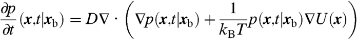
Our mathematical model is diffusion in a potential, U(x), within a bounded domain, , representing the nucleus. We model the specific binding site the protein is searching for as a small absorbing sphere of radius r_b about the point x_b∈Ω. Let D be the diffusion constant of the protein (with units of μm²/s), k_B Boltzmann’s constant, and T temperature (in Kelvin). We denote by p(x,t|x_b) the probability density that the molecule has not yet bound to the binding site, and is located at x∈Ω at time t, given that the binding site is at x_b. The time evolution of p(x,t|x_b) is then given by the Fokker–Planck equation

[1]

for x∈Ω and |x - x_b| > r_b. Note, here the spatial derivatives are with respect to the x coordinate. Although it appears here that we are using a constant diffusion coefficient, see SI Text for a change of variables that leads to an alternate interpretation of Eq. 1.

Let ∂Ω denote the nuclear membrane and η(x) the outward unit normal vector to the membrane at x∈∂Ω. The associated boundary conditions to [1] are then

[2]

[3]

The first, Dirichlet, boundary condition models the binding reaction, whereas the second, Neumann, boundary condition models the assumed impermeability of the nuclear membrane to the regulatory protein.

As described in Materials and Methods, from the data of ref. 1, we were able to reconstruct a triangulated surface representation for the nuclear membrane (see Fig. 1B), and a discrete intensity field for the DAPI stained DNA (see Fig. 1A). Let i = (i₁,i₂,i₃) denote the multiindex labeling the ith voxel of the mesh. (Each two-dimensional image is assumed to lie in a plane perpendicular to the z axis, with each intensity value of a pixel corresponding to the intensity value of a three-dimensional voxel centered in z on the pixel plane.) Based on the data in ref. 1, the voxels were assumed to have spatial dimensions of approximately .0397 by .0397 by .125 μm. We subsequently label these dimensions by h = (h₁,h₂,h₃). Denote by I_i the normalized DAPI stain intensity in the ith voxel, given by [9]. As the imaging data is defined on the mesh given by the collection of voxels, we work with a spatially discrete reaction-diffusion master equation (RDME) model for the motion of the protein (instead of the spatially continuous Fokker–Plank equation [1]).

Fig. 1.

(A) DAPI intensity field reconstructed from data in ref. 1. Note, the volume rendering of the field is partially transparent to allow the viewer to see through it. This effect causes the field to appear sparser than it is in actuality. Movie S2 shows a rotating view of the volume rendering. Axis units are in μm. (B) Surface triangulation of the nuclear membrane. Reconstructed from the fluorescent nuclear pore imaging data of ref. 1 as described in Materials and Methods. Movie S1 shows a rotating view of the surface mesh. Axis units are in μm. The surface triangulation contains approximately 5,000 vertices. Of these, approximately 2,000 are the sites of nuclear pores, the other approximately 3,000 are the result of the triangulation process. The pores are too small to resolve as holes, in the scale of the figure, but the locations of the pores are indicated by small red spheres. (C) Histogram of the probability distribution of intensity values within voxels. Each bar height gives the probability that intensity values fall between the intensity values at the bar’s edges. Note the edges are separated by 0.025 intensity units for each bar. The left y-axis corresponds to the bar heights. A graph of the cumulative distribution function (cdf) for the normalized DAPI fluorescence intensity within voxels is overlaid on the histogram. Let I denote a value of the normalized fluorescence intensity and the random variable for the intensity within an arbitrary voxel. The cdf is the 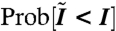. Circles denote every tenth percentile. In our study, binding sites are selected based on these percentiles, as explained in the text. The right y-axis gives the values of the cdf.

Using the Cubes software program (12) we calculated the intersection of the mesh of imaging voxels with the nuclear membrane surface. (See Materials and Methods for details on the resulting embedded boundary mesh.) Denote by x_i the centroid and by V_i the volume of the portion of the ith voxel located within the nucleus. We let A_ij represent the area of the portion of the face separating voxels i and j that is within the nucleus. Finally, we define 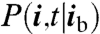to be the probability that the regulatory protein has not yet found its binding site and is within the ith voxel at time t, given that the binding site, x_b, is located within voxel i_b. To obtain an RDME for the time evolution of P(i,t|i_b) we combine the finite volume discretization method of ref. 13 for obtaining RDMEs with pure-diffusive motion, with a discretization method similar to that of ref. 14 for discretizing Fokker–Plank equations (see SI Text for details). The method described in SI Text is used to discretize the spatial fluxes associated with [1], and the resulting expressions are used in the method of ref. 13 to derive the transition rates within the RDME.

We assume that within the voxel, i_b, a binding reaction may occur with bimolecular reaction rate k (having units of μm³/s). In our actual numerical simulations we take k = ∞ so that the protein binds instantaneously upon reaching the voxel, i_b. The “binding times” we subsequently study then represent the time for the protein to first find a small region (with the size of a voxel). This would (approximately) correspond to choosing r_b in [2] to define a spherical binding site with the same volume as a voxel. If we had instead assumed the binding site is substantially smaller than the size of a voxel, we have previously shown (15–17) that the choice k = 4πDr_b makes the solution to the RDME an asymptotic approximation in r_b of p(x,t∣x_b).

The final discretized RDME model we obtain from [1] is then

[4]

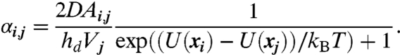
where the jump rates, α_i,j,, give the probability per unit time of the protein hopping from the jth voxel to the ith voxel when the protein is within the jth voxel. These hopping rates incorporate both diffusion and drift due to the potential, U(x). Note that the RDME [4] is a coupled system of ordinary differential equations (ODEs), with one ODE for each voxel location, i. α_i,j will be zero unless voxels i and j are direct neighbors in the dth direction (d = 1, 2, or 3 corresponding to the x, y, and z directions). The jump rates for voxels that are neighbors along the dth coordinate, as determined by our discretization procedure, are

[5]

For voxels that are not cut by the nuclear membrane this expression reduces to

[6]

Note that when the potential at the neighbor, i, is substantially larger than the potential at the current location, j, then the hopping rate from j into i approaches zero. It is more difficult to hop to voxels with higher potential values.

The volume exclusion potential, U(x), was chosen based on the intensity of the DAPI stain within the ith voxel. We assumed that regions of higher DAPI stain intensity should correspond to regions with a higher density of chromatin, and hence be more difficult for a regulatory protein to move into. Several functional relationships between the intensity field and the volume exclusion potential were tried, however, for the remainder we assume a linear scaling,

[7]

Here the scaling constant, , is considered a model parameter that determines the maximum “repulsiveness” of the potential. We subsequently refer to as the “volume exclusivity” of the chromatin. When is zero the regulatory protein will simply diffuse within the nucleus as if the nuclear volume were empty. In contrast, when is large it will be very difficult for the protein to move into regions of high DAPI stain intensity.

Regulatory proteins begin their search process after entering the nucleus through a nuclear pore. Instead of restricting the initial location of the protein to a specific pore or collection of pores, in the model the initial position of the protein was chosen from a uniform distribution among all the pore locations. The probability the regulatory protein was initially in voxel i was therefore

[8]

To study the effect of varying binding site position within different regions of the nucleus, we also allowed the binding site location, i_b, to be a random variable. The set of voxels in which the binding site could be placed were determined by specifying an allowable range of intensity values. For each simulation the voxel representing the binding site was then chosen from a uniform distribution over all voxels having intensity values within the given range. We specified two percentiles of the intensity value distribution, shown in Fig. 1C, to determine an interval of allowable intensities. When choosing lower percentiles, the binding site was prevented from being placed in voxels of very high DAPI stain intensity. This was used to model that such voxels may not contain active binding sites (for example, because these voxels may contain silenced heterochromatin). Similarly, using intervals that only contained nonzero intensity values was used to model that regions of zero, measured, DAPI stain intensity may not actually contain DNA (and hence have no active binding sites).

Numerical Implementation

One method to study the time required for a regulatory protein to find a specific binding site would be to solve numerically the system of ODEs given by the RDME [4]. By allowing i_b to be a random variable, the term δ_i,ib causes [4] to contain a random coefficient. We would therefore need to solve numerically [4] for many choices of i_b sampled from within the range of allowable intensity values. An alternative approach is to simulate instead the stochastic process described by the RDME [4]. This process models the regulatory protein as undergoing a continuous time random walk between voxels, with hopping rates between voxels given by α_i,j. When located in the voxel with the binding site, i_b, the protein may also bind with probability per unit time, k/V_ib. As we took k = ∞ for the simulations of the next section, this corresponded to ending the simulation once the protein hops into the voxel, i_b. Realizations of the stochastic process described by the RDME can be created through the use of the Gillespie method (18) [also known as kinetic Monte Carlo (19)]. With the exception of floating point error in arithmetic operations and the error induced through the use of pseudorandom number generators, the Gillespie method is exact in simulating this stochastic process.

Using the Gillespie method, our numerical simulation algorithm can be summarized as follows

1. Precalculate the jump rates α_i,j.

2. Sample the binding site location, i_b, from a uniform distribution among the voxels within the specified intensity range.

3. Sample the initial position for the protein from P(i,0).

4. Use the Gillespie method to simulate the motion of the protein until the time, T, it binds (i.e., first hops into voxel i_b).

5. Repeat from step 2 until the desired number of simulations have been run.

For certain parameter choices, in a small fraction of simulations, always less than 10^-4, we observed that the protein could take such a long time to find the binding site that for practical purposes the binding site was never found. We believe that this behavior arose for one or more of the following reasons: (i) pure chance, as it is always possible in a stochastic simulation for anything to happen (or in this case fail to happen); (ii) the binding site being chosen in a voxel that is cut off by voxels of high potential from the nuclear pore where the search is chosen to begin; and/or (iii) the trapping of the diffusing protein within regions of high potential that it may happen to enter and have difficulty in exiting. These individual simulations would take several orders of magnitude longer computing time than those in which the protein bound on physically relevant timescales. To avoid computational slow downs, we stopped any simulation where the protein had not bound by a prespecified time, t = T_max. We generally chose T_max to be 10⁷ seconds. In those parameter regimes where a small subfraction of simulations were stopped before binding, our observed values for T represented censored data. Because estimation of the sample median and its standard error is unaffected when the number of censored samples is small, we use the median binding time rather than the mean as an overall measure of the time required to find a binding site. Ninety-five percent confidence intervals of the median were estimated using the PB₂ estimator for the variance of the sample median (20). Survival distribution functions for the probability the binding time random variable, T, is greater than t, Prob[T > t], were estimated using MATLAB’s ecdf routine. Associated 95% confidence intervals were estimated with the same routine.

Results

We now study how the random variable, T, for the time at which the protein first binds to the binding site varies as a function of the maximal potential strength and binding site location. The bimolecular reaction-rate, k, is chosen to be infinite, so that the binding reaction occurs instantaneously upon the protein entering the voxel containing the binding site. This assumption effectively chooses the binding site to be the size of one voxel. Note the model does not account for the kinetics of binding once near the site, or for secondary effects (such as whether the binding site is in an open, binding accessible state (21, 22).

An example illustrating the effect of volume exclusion for a specific initial protein position and binding site location when D = 10 μm²/s is shown in Fig. 2. The specific pore shown in red in Fig. 2A and binding site shown in purple, were used as the initial and binding site positions for all simulations. The continuous time random walk of the protein within the potential [7] was then simulated as described in the previous section. An individual simulation completed when the protein first reached the voxel representing the binding site (and the time, T, at which this occurred was recorded), or was terminated if the the binding time exceeded a maximum time, T_max = 10⁷. Fig. 2A shows a typical trajectory of one protein undergoing the search process (Movie S3 shows the motion of a protein within the volume exclusion potential field).

Fig. 2.

Binding time statistics for a specific fixed initial position and specific fixed binding site when D = 10 μm²/s. (A) A typical path of the protein’s random walk. The red sphere is drawn centered about the centroid of the voxel containing the pore from which the protein began its search. Similarly, the purple sphere is drawn centered about the centroid of the voxel that represented the binding site. The size of the spheres is purely for illustrative purposes. Note the path is a piecewise linear curve connecting the centroids of the voxels in which the protein was located approximately every one hundredth of a second. Between any two points of the path the protein actually underwent many hops between voxels. For this simulation the maximum of the potential was chosen to be 40 k_BT. Movie S3 shows the motion of a protein during the search process. (B) For the binding site position and initial position shown in (A) the probability the protein has not bound at time t as is varied. Note that each line corresponds to statistics determined from 128,000 simulations. The dashed lines above and below each solid line correspond to 95% confidence intervals. Note that the y-axis is a logarithmic scale, showing that the survival probability is approximately exponential in time. (C) Median binding time with 95% confidence intervals as is varied. For each data point 128,000 simulations were run. As the volume exclusivity is increased from zero (no volume exclusion), a minimum median binding time is reached. Beyond about the median binding time increases.

Fig. 2C shows the median time to find the binding site as the magnitude of the volume exclusivity of the chromatin is increased. The graph illustrates that the median binding time decreases as the volume exclusivity is increased, until a minimum binding time is reached. As the volume exclusivity is further increased the median binding time then increases. The same effect is visible in the survival time curves, Prob[T > t], shown in Fig. 2B. Note these curves appear well-approximated by an exponential process (as the curves are linear when the y-axis uses a logarithmic scale). For the rate constant of the exponential is approximately .005 s^-1. Using that the volume of the nucleus is 528 μm³, the binding process can be approximated by a well-mixed reaction with an association rate of 2.63 μm³ s^-1. Given the dependence of this rate on diffusion constant, binding site size, nuclear geometry, and many other factors, this prediction compares favorably with other experimentally determined in vivo association rates. For example, in ref. 23 the binding of glucocorticoid receptor to a tandem array of mouse mammary tumor virus promoter sites within mouse adenocarcinoma cells was studied by fluorescence recovery after photobleaching (FRAP). The authors’ analysis of the FRAP measurements predicts a lower bound on the association rate to a single binding site within the array of approximately .1 μm³ s^-1. An effective diffusion constant for glucocorticoid receptor of 1.2 μm² s^-1 was also predicted from the experimental data. If we assume the association rate is diffusion limited, and hence proportional to the diffusion constant (3), then rescaling the association rate for a diffusion constant of 10 μm² s^-1 gives a lower bound for the association rate of .83 μm³ s^-1.

Fig. 3 shows the statistics of the binding time as a function of both the binding site position and the volume exclusivity, . For each simulation one nuclear pore was chosen randomly from a uniform distribution among all pores, and the protein was initially placed in the voxel containing that pore. Likewise, for each individual simulation the binding site position was chosen from a uniform distribution over all voxels in a given intensity range. For example, “20 to 30” specified that the voxel representing the binding site should be sampled from those voxels with intensity values between the twentieth and thirtieth percentiles of the intensity value distribution (shown in Fig. 1C). The labels “40 to 50” and “70 to 80” were defined similarly. For each intensity range the binding site was localized within, and each value of , 128,000 simulations were run.

Fig. 3.

Statistics of the binding time as a function of the maximum value of the potential, , and binding site position. For each curve D = 10 μm²/s. In all graphs, 20 to 30 denotes that for each simulation the binding site location was sampled from a uniform distribution among voxels with intensity values in the twentieth to thirtieth percentile of all intensity values. The labels 40 to 50 and 70 to 80 correspond to the fortieth to fiftieth percentiles and seventieth to eightieth percentiles respectively. An (S) at the end of a label, such as 20 to 30 (S), denotes that the intensity values were randomly shuffled among the voxels. That is, the values of I_i were randomly rearranged between the voxels within the nucleus. The volume exclusion potential was then generated from this new intensity field, and both were then used in simulations where the protein binding site was restricted to voxels within the twentieth to thirtieth percentiles of intensity values. In all graphs, for each value of 128,000 simulations were run. (A) Survival time distribution, Prob[T > t], for the binding time random variable, T, when using the 20 to 30 binding site distribution. The dashed lines above and below each curve indicate 95% confidence intervals. (B) The median binding times vs. . (C) The same graph, but with the y-axis rescaled to better show the curves that initially decrease to a minimum. Error bars corresponding to 95 percent confidence intervals are shown in (B) and (C), however, they are smaller than the marker size. Each graph shows that when the binding site is localized to regions of low, but nonzero intensity, the binding time initially decreases to a minimum and then increases as the volume exclusivity, , is increased. Note when the DAPI stain intensity values are shuffled in space, or the binding site is moved to regions of higher intensity values, this effect is lost.

Fig. 3A shows several survival time distributions, Prob[T > t], as is varied from zero to 80 k_BT. For these simulations, the binding site position was sampled from those voxels with DAPI stain intensities within the twentieth to thirtieth percentile of intensity values. As the volume exclusivity is increased from zero the binding time distribution initially shifts down and to the left (so that the binding site is found more quickly). Note, however, as the volume exclusivity is further increased the distributions ultimately shift back upward and to the right (so that the binding site is found more slowly). In contrast to Fig. 2B, where both the binding site and initial position were fixed, the survival time curves no longer appear well-approximated by an exponential distribution. This difference arises because the binding site position is no longer fixed as in Fig. 2B, but is instead chosen from a probability distribution. The survival time distributions shown in Fig. 3A are now averages of the survival time distribution for each fixed binding site over all possible binding sites (namely those within voxels in the 20th to 30th percentiles of intensity values).

Fig. 3 B and C show the median binding time as a function of the volume exclusivity. Different curves correspond to different choices of the intensity range the binding site position was sampled from. Fig. 3C is the same graph as Fig. 3B, but with the y-axis rescaled to better show the curves that decrease in value. When the binding site is restricted to the twentieth to thirtieth or fortieth to fiftieth percentiles of intensity values, the protein initially finds the binding site more quickly as the volume exclusivity is increased. That is, the presence of volume exclusion by chromatin helps decrease the time needed for the protein to find the binding site (vs. when there is no volume exclusivity; i.e. ). As is further increased the median binding time ultimately begins to increase. For binding sites within regions of sufficiently low to moderate, but nonzero, DAPI stain intensities we therefore find a minimum binding time for a nonzero value of the volume exclusivity. This indicates that volume exclusion by chromatin may help to speed up the search process of regulatory proteins for active binding sites.

In contrast, when the binding site is restricted to regions of sufficiently high fluorescence intensity, the 70 to 80 curve, this effect is lost. As is increased the time to find the binding site dramatically increases. This result arises because the regions in which the binding sites are now located become substantially more difficult to enter as the chromatin is made more volume excluding.

We next examined whether the spatial structure of the chromatin density was important in the observed decrease in median binding time as a function of the volume exclusivity. To test this question we randomly permuted the fluorescence intensity values among the voxels within the nucleus. This procedure preserved the distribution of intensity values, shown in Fig. 1C, while eliminating the underlying spatial structure of the intensity field. The field was “shuffled” once, and the statistics of the binding time within this new field, and the potential fields associated with it, were then studied. The 20 to 30 (S) curves in Fig. 3 B and C show the effect of the shuffling procedure on the binding time. For these simulations the binding site position was sampled from voxels with intensity values in the new intensity field between the twentieth to thirtieth percentile of all values. Note that within statistical error the binding time simply increases as the volume exclusivity is increased. That is, the previously observed decrease in binding time as a function of volume exclusivity depends on the spatial structure and correlations within the intensity field (and not just on the distribution of intensity values).

The reduction in binding time as the volume exclusivity initially increases from zero, as shown in Figs. 2C and 3 B and C, is the principal result of this paper. The abolition of this effect by shuffling the voxel intensity values (see curves labeled “S” in Fig. 3 B and C) shows that this reduction in binding time is not merely a consequence of a reduction in the total volume that needs to be searched, but in fact depends on the spatial structure of chromatin, and indeed on some aspect of the spatial structure on a scale that can be resolved with the voxel size used here. Although our results do not reveal specifically what feature of the spatial structure of chromatin is responsible for this effect, we may speculate that the chromatin geometry partitions the three-dimensional intranuclear space into something like a network of one-dimensional channels. This would be significant because of the disparity between the time to find a target by diffusion in the one-dimensional case in comparison to the substantially greater amount of time that is required in higher dimensions (see SI Text). We emphasize, however, the speculative nature of this interpretation of our computational results.

Conclusions

We developed a mathematical model to study how the time required for a protein to find a specific binding site varies as a function of volume exclusion by chromatin and binding site location. The model suggests that binding sites located within regions of small, but nonzero, DAPI stain intensity are found most quickly when chromatin has some, but not too much, volume exclusivity. Randomly shuffling the DAPI stain intensity values among the voxels within the nucleus caused this behavior to disappear. This suggests the macroscopic distribution of chromatin density within the nucleus may be arranged to help funnel proteins toward binding sites within regions of euchromatin (where we expect the chromatin density to be lower). In contrast, binding sites located within regions of high DAPI stain intensity are found most quickly when no volume exclusion is modeled. Because such regions are more likely to contain silenced heterochromatin, it may be less important to optimize chromatin distribution to make them accessible to binding proteins.

Materials and Methods

As input, our model makes use of the structured illumination microscopy data of ref. 1, specifically supplementary movie 1 of ref. 1. From the movie, we were able to reconstruct a nuclear membrane surface and an intensity field for the DAPI stained DNA fluorescence within an individual mouse C2C12 cell nucleus. The movie was split into a collection of images, each corresponding to a slice plane perpendicular to the z-axis of the cell nucleus. Two types of fluorescent data were present in each frame: green “dots” from fluorescently labeled nuclear pores, and a magenta field representing DAPI stained DNA (chromatin).

Nuclear Membrane Reconstruction.

The MATLAB Imaging Toolbox was used to segment and then find the centroid of each nuclear pore. This generated a noisy point cloud representing the locations of the nuclear pores within the cell. Because (functional) nuclear pores are localized to the nuclear membrane, and are generally well distributed over the surface of the membrane and present in large numbers (order of thousands), the point cloud gave a good approximation to the membrane’s location. After removing extreme outliers, most likely fluorescent components of the nuclear pore that were present in other locations within the cell, the implementation of the eigencrust algorithm of ref. 24 distributed in ref. 25 was used to generate a watertight triangulated surface from the point cloud. The resulting surface was cleaned and postprocessed in MeshLab (26). Fig. 1B and Movie S1 show the final triangulated nuclear membrane surface. The mesh is comprised of approximately 5,000 nodes and 9,700 triangles.

DAPI DNA Intensity Field.

Let i = (i₁,i₂,i₃) label the three-dimensional voxel corresponding to pixel (i₁,i₂) in the i₃th image frame. The pixel plane is assumed to be centered within the voxel, perpendicular to the z axis. A three-dimensional DNA fluorescence intensity field, I_i, was created from the DAPI stain intensity values for each pixel. The intensity field was normalized to have values in [0,1] by setting

[9]

Fig. 1A and Movie  S2 show a volume rendering of the resulting discrete DNA fluorescence intensity field, I_i. Note, the rendering is semitransparent to allow the viewer to see within the field. This causes the field to appear to be “clumpier” than it actually is, see the original imaging data, supplemental movie 1 of ref. 1.

Embedded Boundary Cartesian Mesh Derived From Imaging Data.

The three-dimensional voxels centered about the pixels of the image slices define a natural Cartesian mesh. The discretization procedure of the Mathematical Model section requires the calculation of the portion of each voxel that is within the nucleus. Using the Cubes (12) software program the intersection of the reconstructed nuclear membrane surface with this Cartesian mesh was calculated.

References

- 1.Schermelleh L, et al. Subdiffraction multicolor imaging of the nuclear periphery with 3D structured illumination microscopy. Science. 2008;320:1332–1336. doi: 10.1126/science.1156947. [DOI] [PMC free article] [PubMed] [Google Scholar]
- 2.Halford S. An end to 40 years of mistakes in DNA-protein association kinetics? Biochem Soc T. 2009;37:343–348. doi: 10.1042/BST0370343. [DOI] [PubMed] [Google Scholar]
- 3.Smoluchowski MV. Mathematical theory of the kinetics of the coagulation of colloidal solutions. Z Phys Chem. 1917;92:129–168. [Google Scholar]
- 4.Berg OG, Winter RB, von Hippel PH. Diffusion-driven mechanisms of protein translocation on nucleic acids. 1. Models and theory. Biochemistry. 1981;20:6929–6948. doi: 10.1021/bi00527a028. [DOI] [PubMed] [Google Scholar]
- 5.Li GW, Berg OG, Elf J. Effects of macromolecular crowding and DNA looping on gene regulation kinetics. Nat Phys. 2009;5:294–297. [Google Scholar]
- 6.Malherbe G, Holcman D. The search kinetics of a target inside the cell nucleus. 2007 arXiv:0712.3467v1 [q-bio.BM] [Google Scholar]
- 7.Slutsky M, Mirny LA. Kinetics of protein–DNA interaction: Facilitated target location in sequence-dependent potential. Biophys J. 2004;87:4021–4035. doi: 10.1529/biophysj.104.050765. [DOI] [PMC free article] [PubMed] [Google Scholar]
- 8.Mirny L, et al. How a protein searches for its site on DNA: The mechanism of facilitated diffusion. J Phys A-Math Theor. 2009;42:1–23. [Google Scholar]
- 9.Elf J, Li G, Xie XS. Probing transcription factor dynamics at the single-molecule level in a living cell. Science. 2007;316:1191–4. doi: 10.1126/science.1141967. [DOI] [PMC free article] [PubMed] [Google Scholar]
- 10.Bancaud A, et al. Molecular crowding affects diffusion and binding of nuclear proteins in heterochromatin and reveals the fractal organization of chromatin. EMBO J. 2009;28:3785–3798. doi: 10.1038/emboj.2009.340. [DOI] [PMC free article] [PubMed] [Google Scholar]
- 11.Vargas DY, Raj A, Marras SAE, Kramer FR, Tyagi S. Mechanism of mRNA transport in the nucleus. Proc Natl Acad Sci USA. 2005;102:17008–13. doi: 10.1073/pnas.0505580102. [DOI] [PMC free article] [PubMed] [Google Scholar]
- 12.Berger MJ. Cubes AMR Embedded Boundary Meshing Program [Google Scholar]
- 13.Isaacson SA, Peskin CS. Incorporating diffusion in complex geometries into stochastic chemical kinetics simulations. SIAM J Sci Comput. 2006;28:47–74. [Google Scholar]
- 14.Wang H, Peskin CS, Elston TC. A robust numerical algorithm for studying biomolecular transport processes. J Theor Biol. 2003;221:491–511. doi: 10.1006/jtbi.2003.3200. [DOI] [PubMed] [Google Scholar]
- 15.Isaacson SA. The reaction-diffusion master equation as an asymptotic approximation of diffusion to a small target. SIAM J Appl Math. 2009;70:77–111. [Google Scholar]
- 16.Isaacson SA, Isaacson D. Reaction-diffusion master equation, diffusion-limited reactions, and singular potentials. Phys Rev E. 2009;80:1–9. doi: 10.1103/PhysRevE.80.066106. [DOI] [PMC free article] [PubMed] [Google Scholar]
- 17.Isaacson SA. Relationship between the reaction-diffusion master equation and particle tracking models. J Phys A-Math Theor. 2008;41:1–15. [Google Scholar]
- 18.Gillespie DT. Exact stochastic simulation of coupled chemical-reactions. J Phys Chem. 1977;81:2340–2361. [Google Scholar]
- 19.Bortz AB, Kalos MH, Lebowitz JL. A new algorithm for Monte Carlo simulation of Ising spin systems. J Comp Phys. 1975;17:10–18. [Google Scholar]
- 20.Price RM, Bonett DG. Estimating the variance of the sample median. J Stat Comput Sim. 2001;68:295–305. [Google Scholar]
- 21.Li G, Levitus M, Bustamante C, Widom J. Rapid spontaneous accessibility of nucleosomal DNA. Nat Struct Mol Biol. 2004;12:46–53. doi: 10.1038/nsmb869. [DOI] [PubMed] [Google Scholar]
- 22.Poirier MG, Bussiek M, Langowski J, Widom J. Spontaneous access to DNA target sites in folded chromatin fibers. J Mol Biol. 2008;379:772–786. doi: 10.1016/j.jmb.2008.04.025. [DOI] [PMC free article] [PubMed] [Google Scholar]
- 23.Sprague BL, et al. Analysis of binding at a single spatially localized cluster of binding sites by fluorescence recovery after photobleaching. Biophys J. 2006;91:1169–1191. doi: 10.1529/biophysj.105.073676. [DOI] [PMC free article] [PubMed] [Google Scholar]
- 24.Kolluri R, Shewchuk J, O’Brien J. Spectral surface reconstruction from noisy point clouds; SGP ’04: Proceedings of the 2004 Eurographics/ACM SIGGRAPH Symposium on Geometry processing; 2004. pp. 11–21. [Google Scholar]
- 25.Kolluri R. Eigencrust Software. Available in the MATLAB PointCloudToolbox at http://bdtnp.lbl.gov/Fly-Net/bioimaging.jsp?w=pcml.
- 26.3D CoForm Project. MeshLab. Available from http://meshlab.sourceforge.net/
- 27.Lawrence Livermore National Lab. Visit Visualization Software. Available at https://wci.llnl.gov/codes/visit/home.html.
Associated Data
This section collects any data citations, data availability statements, or supplementary materials included in this article.