

Abstract
Because the space of folded protein structures is highly degenerate, with recurring secondary and tertiary motifs, methods for representing protein structure in terms of collective physically-relevant coordinates are of great interest. By collapsing structural diversity to a handful of parameters, such methods can be used to delineate the space of designable structures, i.e. conformations that can be stabilized with a large number of sequences – a crucial task for de novo protein design. We first demonstrate this on natural α-helical coiled coils using the Crick parameterization. We show that over 95% of known coiled-coil structures are within 1 Å Cα root mean square deviation of a Crick-ideal backbone. Derived parameters show that natural geometric space of coiled coils is highly restricted and can be represented by “allowed” conformations amidst a potential continuum of conformers. Allowed structures have 1) restricted axial offsets between helices, which differ starkly from parallel to anti-parallel structures; 2) preferred superhelical radii, which depend linearly on the oligomerization state; 3) pronounced radius-dependent a and d-position aminoacid propensities and 4) discrete angles of rotation of helices about their axes, which are surprisingly independent of oligomerization state or orientation. In all, we estimate the space of designable coiled-coil structures to be reduced at least 160-fold relative to the space of geometrically feasible structures. To extend the benefits of structural parameterization to other systems, we developed a general mathematical framework for parameterizing arbitrary helical structures, which reduces to the Crick parameterization as a special case. The method is successfully validated on a set of non coiled-coil helical bundles, frequent in channels and transporter proteins, which show significant helix bending but not supercoiling. Programs for coiled-coil parameter fitting and structure generation are provided via a web interface at http://www.gevorggrigoryan.com/cccp/, and code for generalized helical parameterization is available upon request.
Keywords: designability, protein design, structural parameterization, coiled coils, Crick parameterization
1. Introduction
The number of conformational states accessible to even small proteins is astronomically large. Nevertheless, the space of natively folded protein structures is rather limited in comparison, with highly recurring secondary and tertiary motifs. Clearly, simple physical principles, such as volume exclusion or electrostatic repulsion, preclude many structures. However, beyond this simple filter, natively folded structures are much more restricted due to other requirements imposed by biology, including robustness of the fold in sequence space[1, 2]. In the context of folding and inverse folding problems, structure robustness in sequence space has been referred to as designability[3, 4, 5]. Natural abundance of structures and their designability are related. Structural motifs that recur frequently in nature must be able to accommodate a reasonably wide ensemble of sequences and are thus designable. Koehl and Levitt have shown that the designability of a protein structure, measured as the number of sequences compatible with its backbone in an atomistic-level in silico protein design experiment, correlates well with its evolutionary designability, as assessed with sequence bioinformatic tools[6]. Kuhlman and Baker demonstrated that the evolutionary sequence profile of the SH3 domain can be recapitulated from a small collection of SH3-domain backbones via computational protein design[7].
Finding the relationship between structure and designability is a fundamental problem in protein design, as one would like to a priori limit oneself to engineering only reasonably designable structures. However, such a relationship is difficult to synthesize because of the very large number of parameters required to exactly define the geometry of a protein. Thus, approaches for representing folded structures via a reduced set of effective parameters can greatly facilitate this process. One class of such methods, which we will refer to as ideal backbone parameterization, are particularly well suited for this task. These approaches model the overall shape into which secondary-structure elements fold with a few parameters, and can often capture the majority of observed structural variability, producing deviations between ideal and real structures within 1 Å. Examples of this include the Crick parameterization of coiled coils[8, 9], mathematical description of β-barrel structures[10, 11], statistical parameterization of the structure of collagen[12], parameterization of di-iron helical bundles[13] and transmembrane helix interaction geometry[14, 15]. Such methods have been quite useful in de novo protein design[16, 17, 18, 19, 20, 21], modeling of thermodynamic consequence of mutations[21], protein-protein interaction prediction[22, 23], structure prediction and modeling[24, 25, 14, 15], and X-ray crystallography[26].
Recent studies of designability, using lattice models and native protein structures, suggest that more designable folds are those that have more contacts per residue (contact density)[4, 6, 27, 1, 28, 5, 4], and that more designable structures also tend to be more thermodynamically stable[1, 4]. These important findings further our understanding of designability of different folds and choice of fold by evolution. Such studies can be thought of as an instance of structural parameterization with the goal of relating it to designability. Contact density and on-lattice models provide a coarse view, appropriate for differentiating folds from one another in the global structure space. Here we are concerned with a more fine-grained description of variability within a given fold, and so a higher-resolution, but nevertheless low-parameter description of designability is sought. For de novo protein design, such a detailed description of designability is often needed, as this information is critical for the choice of target template coordinates.
Here we aim to quantify the constraint of designability on the space of natural helical bundles, starting with the coiled coil. Others have shown that the Crick parameterization can closely fit natural coiled-coil backbones[23, 9, 16, 29, 30]. In fact, we demonstrate that it can reproduce to within 1 Å Cα root mean square deviation (RMSD) over 95% of all available coiled-coil structures, with a median RMSD of 0.44 Å. Further, sharp distributions of Crick parameters indicate significant biases in the space of naturally designable structures. For example, axial offsets between helices are restricted to a small range relative to the space of geometrically possible offsets, and these allowed regions differ strongly between parallel and anti-parallel helix pairs. Overall, we estimate that the space of designable structures is at least 160 fold smaller in relation to the space of geometrically reasonable structures, illustrating the importance of considering designability a priori in protein engineering applications.
The Crick parameterization has been difficult to extend to helical bundles in general, due to their less regular structure, in which each chain is not necessarily identical and the implied symmetry is difficult to observe. While a trained eye may be able to discover residual symmetry underlying considerable complexity[13, 31], it has been difficult to do this in an objective and automated manner. Moreover, there are a continuum of helical bundles, ranging from the very regular coiled-coils, to ones that are less regular and defy simple canonical categorization. In general, helical bundles form with relatively well-defined and recurring helix-crossing angles that reflect the restraints associated with achieving good side-chain packing at the local level[32, 33, 34, 35, 36] (see Figure 2). Early work by Murzin and Finkelstein showed that helices in globular helical proteins tend to lie approximately along the ribs of certain close-to-spherical polyhedra[34]. Due to the non-integral nature of the alpha-helix, good packing generally does not occur when helices are packed with their axes precisely parallel or anti-parallel to one another. Instead, side-chain packing tends to be optimized when the helical axes are at an angle to one another, resulting in the divergence of straight helices. Supercoiling, as observed in coiled coils, reflects the resolution of the frustration between optimizing interactions locally versus globally over the entire structure. Shorter helical bundles, however, do not necessarily form coiled coils. Indeed, natural divergence of straight helices can form important functional pockets, or the helices can bend or kink in more complex manners. These articulation points can serve as hinges for functional motions involved in signaling, gating, and ion conduction[37].
Figure 2. Common types of helical bundles.

Generally, helical bundles form via relatively well-defined and recurring motifs. The classical diverging straight-helix bundle shown in A) is from the structure E. coli PhoQ sensor domain (PDB code 3BQ8). The bundle shown in B) (from bacteriophytochrome chromophore binding domain, PDB code 2O9C) also diverges, but the individual helices are bent into circular arcs and do not wrap around each other like in coiled coils. This motif can be thought of as a first-order generalization of the classical straight-helix diverging bundle. Shown in C) is the left-handed coiled-coil domain from the yeast transcription factor GCN4 (PDB code 2ZTA). The helical wheel diagram on the left illustrates the seven-residue heptad repeat commonly characteristic of left-handed coiled coils. Positions a and d are in the core and often occupied with hydrophobic amino acids, e and g are along the interface, often forming salt bridges and polar interactions, and b, c, and f adjust to the environment. Although significantly less common, right-handed coiled coils also occur, such as the example shown in D) from the human VASP tetramerization domain (PDB code 1USE). Boxed insets represent an alternative view of each bundle.
As a second goal of this work, we develop a general ideal backbone parameterization approach for arbitrary helical structures. This mathematical framework describes α-helices forming any superstructure defined via a 3-D parametric curve, and reduces to the Crick parameterization in the special case when the parametric curve is itself a helix. The generalized framework provides significant simplification of structural representation, while still capturing natural structural variability. We illustrate this using a helical bundle motif common in membrane channels and signaling proteins. This motif consists of helices that curve into nearly perfect circular arcs to form a bundle, but do not wrap around each other like coiled coils. Such structures appear as inner and outer bundles lining channel pores (in fact, they are present in virtually all channel families, as defined by the OPM database[38]) and oligomerization interfaces of bacterial signaling proteins. Our parameterization is able to fit such native bundles with Cα RMSD of better than 1.0 Å in 52 of the 55 representative examples analyzed. These findings are particularly significant in light of the functionally important regions of structure these bundles are found in, introducing the potential that functionally-relevant structural changes may be modeled and understood in terms of simple geometric parameters.
2. Results
Coiled-coil structures from the CC+ database[39] longer than 11 residues (see Materials and Methods for details) were analyzed using our automated program CCCP (Coiled-Coil Crick Parameterization) for fitting coiled-coil backbones. The modified Crick equations used in CCCP allow for anti-parallel and mixed orientations and for helical sliding with respect to the interfacial axis (see Materials and Methods). For 95.7% of the analyzed structures Cα root mean square deviation (RMSD) between ideal and native structures was below 1.0 Å and the performance did not significantly depend on the orientation or oligomerization state (see Figure 3 for error distributions). The error did, however, depend on structure size, increasing roughly linearly with the total number of residues fit up to ~ 0.9Å. This is not surprising as small local deviations from ideality can lead to large deviations over long distances.
Figure 3. Distribution of fitting error.
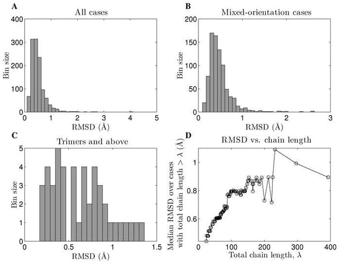
A) The distribution of fitting error (Cα RMSD between a natural structure and its Crick-parameterized version) over all cases. Four structures were fit with RMSD above 2.0 Å, but in 95.7% of cases the RMSD was below 1.0 Å. B) The distribution of fitting error for cases where helices of opposite orientation were present (i.e. anti-parallel dimers and mixed-orientation higher-order oligomers). The performance on these structures is not significantly different from the overall performance. C) Distribution of fitting error for trimers, tetramers and pentamers. D) Fitting error as a function of the total number of residues fit. The y-axis shows the median Cα RMSD over cases where the total number of residues fit was above the corresponding value on the x-axis.
The set of coiled coils with known structure contains a significant amount of redundancy, whereby some sequence families (or, in some cases, many mutants of the same sequence) are significantly over-represented. To ensure that our analysis was devoid of such biases, we filtered the dataset down to less than 50% sequence redundancy, resulting in 868 structures (see Materials and Methods). All further analysis was performed on this dataset. The analysis of error distribution was repeated for this subset and resulted in virtually identical trends (see Supplementary Figure S2).
2.1. Superhelical Radius
The distribution of superhelical radii is shown in Figure 4. Several sub-populations are apparent and these correspond to different oligomerization states (see figures 3B–D). The medians of the sub-populations (4.85, 6.36, 7.30 and 8.59 Å for dimers, trimers, tetramers and pentamers, respectively) correlate nearly perfectly with oligomerization state with the best fit line R0 = 1.24 · n + 2.4 (RMSD 0.1 Å, see Supplementary Figure S3), where n is the oligomerization state. This indicates that the inter-helical distance, which can be expressed as (limiting value of 1.24 · 2 · π ≈ 7.8Å), decreases with increasing oligomerization state above dimer.
Figure 4. Distribution of superhelical radius.
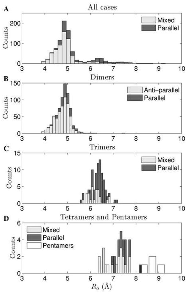
Stacked bar plots show the the overall distribution of R0 (total histogram) as well as contributions to it from structures of parallel orientation (dark gray bars) and anti-parallel or mixed orientation (light gray bars). A) The distribution of R0 is multi-modal with peaks corresponding to different oligomerization states. B)-C) Show distributions of R0 for dimers and trimers, respectively, and D) combines tetrameric and pentameric cases (of the four pentameric structures, all are of parallel orientation). The median values of the distributions are 4.85 Å for dimers, 6.36 Å for trimers, 7.30 Å for tetramers and 8.59 Å for pentamers.
One of the restrictions of the Crick parameterization is that the superhelical radius (R0) is assumed to be constant throughout the structure. We wondered to what degree R0 actually does change in natural structures. To that end, for dimers longer than three heptads, we compared the value of R0 obtained by fitting the entire structure to values obtained by fitting individual two-heptad windows scanned across the structure (see Supplementary Figure S4). In most cases, local and global R0 coincide closely (median deviation is 0.1 Å), however, exceptions to this do exist, especially for long structures (Supplementary Figures S4 and S5). The highest observed rates of superhelical radius change are around 0.14 Å per residue. The median auto-correlation length of R0 is seven residues (defined in Materials and Methods), indicating that the structure has some memory of the superhelical radius for about a heptad.
Even though variations of R0 within an oligomerization state are small, we wondered whether these correlate with amino-acid composition of core a and d positions. To test this, we considered two simple models for the dependence of R0 on the core composition. In the first, superhelical radius depends linearly on the composition of a and d positions and in the second, amino acids with the largest radius preferences determine the value of R0 (see Materials and Methods for details). Fitting local R0 values to either model leads to a weak agreement such that roughly 20% of the observed superhelical radius variability can be attributed to either of these simple expressions (see Supplementary Figure S6). Sequence context likely plays a significant role in determining which aspects of the local coiled-coil geometry are perturbed upon changes in the identity of core amino acids (e.g. axial sliding of chains, changes in side-chain rotameric states or adjustments in helical and superhelical phases).
On the other hand, amino acids at a and d may still have pronounced radius preferences, even though a/d composition alone may not amount to a quantitatively predictor of local R0 variation. To measure these preferences, we considered a subset of the dimeric two-heptad segments described above, in which either position a or position d were in the center and which had parallel orientation. The superhelical radii of these segments were then studied in relation to the amino acids occupying the central a or d position. All segments were binned by value of R0. Next, for each amino acid occurring at either the central a or d positions, the frequency of its occurrence in each bin was calculated and normalized by the overall frequency of the amino acid in the coiled-coil database, to arrive at amino-acid specific propensities for different radii. To minimize noise from statistics of small numbers, for a given amino acid aai, bins with very few occurrences of aai were grouped with neighboring bins and the average number of counts was assigned to each bin of the group when computing propensities for aai. Figure 5 shows the resulting propensities for the top ten most frequent amino acids at either the a or d positions, respectively. In these plots, amino acids are ordered, left to right and top to bottom, in the order of decreasing frequency of occurrence at the respective position (e.g. the first four most frequent at a are Leu, Ile, Val, and Asn, in that order).
Figure 5. a/d-position amino-acid superhelical radius propensities.
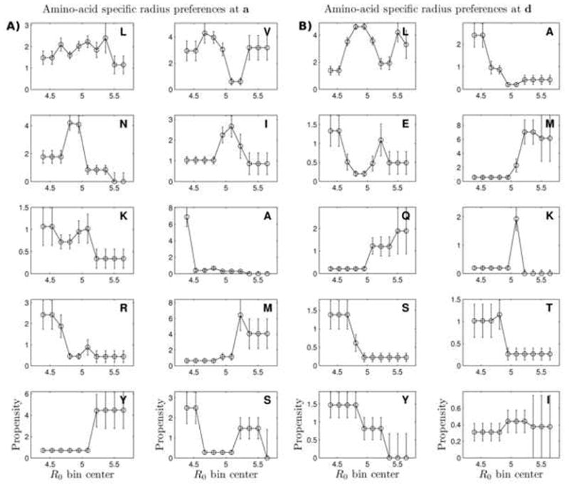
Two-heptad windows of dimeric structures were considered in which a (in panel A) or d (in panel B) positions were in the center. Values of R0 obtained by Crick parameter fitting were divided into ten equally spaced bins. For every amino acid aai values plotted as a function of superhelical bin bj are , where N (aai, bj) is the number of occurrences of aai in bin bj, Ntot is the total number of data points, faai is the frequency of aai in the entire dataset, and fbj is the fraction of structures with a superhelical radius within bin bj. To correct for low counts, bins with the number of counts of a particular amino acid below three where grouped with neighboring bins until the total number of counts became above three, and the average number of counts over the group was assigned to each bin within the group. Error bars designate the error of determination of each propensity and were computed by considering all possible binomial distributions that could have given rise to the observed number of successes k = N (aai, bj) out of the number of trials N = Ntot · fbj, and calculating the error expectation as: , where p is the probability of success of the considered binomial distribution, Pb (k, N, p) is the binomial probability density of k successes from N trials and a success probability of p, and p̄ is the expectation of p given k successes and N trials, or .
At the a position, Leu appears to be the most malleable amino acid as it is widely accommodating of a large range of radii. Leu is also the most common amino acid at this position, which, in part, helps explain why the precise local deviation of the superhelical radius from its characteristic value cannot be easily predicted purely from the composition of core amino acids. Val, Asn and Ile, by contrast, appear much more specialized for particular radius ranges, especially pronounced in the case of Asn and likely due to its strong preference to pair with another Asn at a′. Ala, not surprisingly, shows an extremely strong preference for small radii and so do Lys and Arg, though with a considerably lower magnitude of the preference. As the number of observations of a particular amino acid decreases, statistical error grows, but the preference of Tyr and Met for larger radii is consistent with their sterics. Like at the a position, at d Leu occurs in a wide range of radii and Ala shows strong preference for small radii (see Figures 5B). The amino-acid alphabet is much more restricted at d, compared to a, with Leu and Ala amounting to 60% of all cases (whereas it takes the top four amino acids at a to get to 60%), so statistics fall off rapidly after Ala, as indicated by larger error bars in Figures 5B.
2.2. Superhelical Frequency and Pitch Angle
Superhelical frequency (ω0) determines the degree of twist of the superhelix. That is, for every residue, the angle by which the superhelix turns around the coiled-coil axis is ω0. Values around −3.6°/res are considered canonical (the negative sign indicates a left-handed superhelix) such that the superhelix completes a full turn in 100 residues. This parameter is tied to the superhelical radius via the relationship:
| (1) |
where ω0 is in radians, α is the pitch angle and d is the rise per residue. The latter is the arc length along the superhelical curve from one residue to the next. In a straight helix that is aligned along the Z-axis, d is just the displacement in the Z-direction from one residue to the next. This is roughly 1.51 Å for an ideal α-helix. Superhelical parameters that result in d significantly different from its ideal value correspond to cases where the alpha helix is locally strained (e.g. stretched or compressed). This places restraints on the product R0ω0, such that for any given radius the absolute value of ω0 can vary between 0 (corresponding to straight aligned helices) and roughly (in radians per residue).
Figure 6A shows the distribution of ω0 observed in the structural dataset. The range of absolute values is between 0 and 8.7°/res and the median of the distribution is −3.5°/res, meaning that the most tightly wound coiled coil has a period of about 41 residues (since the period is residues) and the average coiled coil completes its period in roughly 102 residues. As expected, the overwhelming majority of annotated coiled coils are left-handed (negative ω0). In fact, only seven unique structures in the CC+ database showed a significant overall right-handed character, among which are RH4 and RH4B – coiled coils designed to be right-handed[18, 40]. It was formally possible that the number of right-handed structures in CC+ was unfairly reduced due to a possible bias in the program SOCKET[41] for recognizing the type of knobs-into-holes packing more characteristic of canonical left-handed structures. We therefore performed Cα distance matrix-based structural similarity searches of the entire PDB (see Materials and Methods for details) as well as keyword-based searches of the PDB and the literature to look for additional right-handed coiled-coil structures. In so doing, we uncovered five more clear examples of right-handed bundles with supercoiling and included these in all of our analyses. Although none of the above methods likely recover all available examples of right-handed coiled coils, the significantly lower rate of discovering right-handed versus left-handed coiled coils in the structural database, argues that right-handed coiled coils are significantly less common and likely less designable. Within the structures annotated in CC+ there are examples of local right-handed character in coiled-coil packing (such as in a fragment of the Staphylothermus marinus surface layer protein tetrabrachion[42]), whereas Figure 6A shows values of ω0 optimal for entire coiled-coil regions. In a separate set of fits, performed to study the local variation of parameters, we considered two-heptad windows that were scanned along all dimeric coiled coils. This resulted in over 3,000 separate two-heptad fragments, out of which 4.8% best fit with a positive value of ω0.
Figure 6. Distribution of superhelical frequency and pitch angle.

Distributions of superhelical frequency (ω0) and pitch angle (α) are shown in A) and B), respectively. The median and the mean values for ω0 are −3.5°/res and −3.6°/res, respectively, corresponding to a superhelical repeat of about 100 residues or pitch of approximately 150 Å. The median and the mean values for α are −11.9° and −12.0°, respectively.
Figure 6B shows the observed distribution of pitch angles α, that is the angle between a tangent to the superhelical curve and the coiled-coil axis. Once again, this is not a completely free parameter and is related to R0 and ω0 via equation 1. The peak of the distribution is at around 12°. For both pitch angle and superhelical frequency, the peak values are very close to the values that best fit the coiled-coil region of the yeast transcription factor GCN4[43] – the first high-resolution structure of a parallel dimeric coiled coil as well as one that has has long served as the prototypical coiled-coil example. It is interesting that in Crick parametric terms, this structure is indeed prototypical.
2.3. Helical Axial Shift
As outlined in Materials and Methods, we modified the classic Crick parameterization to allow for a helical sliding along the interfacial axis. Thus, in a given structure, each helix after the first one is assigned a value of ΔZoff relative to the first helix. ΔZoff between two helices is defined as the distance along the interfacial axis between the most inward-facing points on the helical curves of the two helices (not necessarily representing Cα atoms; see Figure 1 and Materials and Methods). This definition makes ΔZoff independent of helical phase, rendering it a convenient parameter for sampling and fitting. Interestingly, the distribution of ΔZoff strongly depends on whether the helix pairing in question is parallel or anti-parallel (see Supplementary Figure S7). Whereas for parallel alignments ΔZoff tends to cluster tightly around 0, corresponding to helices with turns Z-aligned at the interface, for anti-parallel alignments, the distribution is much more broad and has two maxima at around ± 2.0–2.5 Å, corresponding to helices with interdigitated turns (the sign of ΔZoff indicates direction of the axial shift, with the positive sign corresponding to the direction shown in Figure 1).
Figure 1. Visual representation of parameters used in coiled-coil fitting.

Geometrical meanings of the superhelical radius (R0), the helical radius (R1), the superhelical frequency (ω0), the helical frequency (ω1), chain axial offset (ΔZoff), chain superhelical phase offset (Δφ0), and starting helical phase (Δφ1) are shown. The green tube represents the interfacial axis. Orange curves depict local helical axes, which in a coiled coil form a superhelix. The gray tube represents the helical curve, which passes through Cα atoms. Orange balls show the inward-facing points on the helical curves (not necessarily corresponding to locations of atoms) defined as points with helical phase equal to π. The distance along the interfacial axis between an inward-facing point on one helix and its closest counterpart on the opposite helix is defined as ΔZoff, with sign indicating the order of the two points, relative to N→C of the first helix. The depicted case is an anti-parallel coiled coil with a positive ΔZoff of 2.4 Å.
To allow for an easier interpretation of axial offset in terms of coiled-coil geometry, CCCP additionally calculates the parameter ΔZaa′ (not used in the fitting), defined as the axial offset between an a position on one helix and the closest a′ position on the interacting helix. Sign of ΔZaa′ indicates whether the closest a′ is downstream (e.g. in the N→C direction of the first chain, corresponding to a positive sign) or upstream (e.g. opposite to N→C direction of the first chain, corresponding to a negative sign). Given its definition, ΔZaa′ can vary between plus and minus half a helical pitch, roughly (where ω1 and d are the helical frequency and rise per residue, respectively) or [−5.3, 5.3] Å for a typical coiled coil. Figure 7 shows that the distribution of ΔZaa′ strongly depends on the mutual orientation of the pair of helices. Parallel coiled-coil helix pairs prefer to line up opposing a positions with a roughly zero axial offset, whereas anti-parallel pairs prefer to interdigitate. Parameter ΔZaa′ further tells us that anti-parallel coiled coils interdigitate in an asymmetric manner with respect to the heptad, such that a given a position is usually closer to the a′ residue downstream of it rather than the upstream a′ residue. In fact, a very large range of ΔZaa′ values, roughly from −5 to 1 Å is unpopulated, narrowing the designable space of anti-parallel coiled-coil backbones. It is common to think of anti-parallel coiled coils as roughly aligning a positions of one chain with d′ positions of the opposing chain. The distribution of the axial offset between a and the closest d′ is shown in Supplementary Figure S8. It is clear that in anti-parallel pairs, a and the opposing d′ positions are rarely exactly aligned, and the closest d′ tends to be upstream of a, with only a minority of structures displaying the opposite alignment.
Figure 7. Distribution of ΔZaa′.
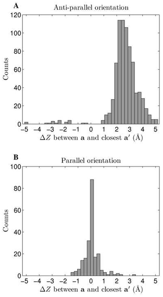
Helix pairs from complexes of all oligomerization states and orientations were considered. The distribution of ΔZaa′ is shown for A) anti-parallel pairs and B) parallel pairs.
2.4. Minor helical phase φ1 and frequency ω1
Helical frequency ω1 characterizes the angular rotation of the α-helix around its local axis with each residue. For an ideal straight helix, this value is 100°/res, such that a full turn of the α-helix is completed in 3.6 residues. In a canonical coiled coil, ω1 is around 102.8°/res, so a complete turn is made in 3.5 residues and two turns in 7 residues. This gives rise to the well-known heptad repeat, commonly denoted with positions a through d (see Figure 2C). In agreement with this, the distribution of ω1 within the coiled-coil structures analyzed amounts to a normal distribution with a mean of 102.8°/res and a standard deviation of only 1.1° (data not shown). Variations in parameter ω1 to a significant extent reflect changes in ω0 (e.g. changes in the reference frame defining a complete helical turn), as opposed to reflecting changes in α-helical geometry (ω1 and ω0 anti-correlate with a correlation coefficient of R = −0.7).
Parameter φ1 in Crick equations (see Materials and Methods) measures the starting angular register, or helical phase, of the α-helix and the helical phase of the i-th residue is given by φ1 + (i − 1) · ω1. Phase values of 0 and π mean that the Cα atom of the residue points directed away from or towards the interfacial axis, respectively. Phase can be used to determine the heptad position assignment of each residue and CCCP does so automatically. Figure 8 shows the distribution of helical phases for residues in all dimeric coiled coils considered in this study. Empty and filled circles show residue phases as the angular coordinate in the polar-coordinate plot, with each point corresponding to a single residue within a single structure. Empty circles represent anti-parallel structures while the filled ones are from parallel structures. The solid line in Figure 8 shows the histogram of helical phase distribution. The seven clearly visible peaks are centered around: 41°, 95°, 146°, 197°, 249°, 300°, and 351°, corresponding to heptad positions c, g, d, a, e, b, and f, respectively (the helix in the figure is shown in the C→N projection). Although actual phase values can vary around these numbers, the peaks of the distribution are fairly narrow with standard deviations around 8°, indicating that heptad positions correspond to well-pronounced minima in the coiled-coil energy landscape.
Figure 8. Distribution of minor-helical phase φ1 in polar coordinates for dimers.
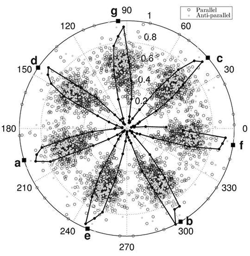
Open and filled circles represent parallel and anti-parallel structures, respectively, with each point corresponding to a single residue within a single structure (to avoid redundancy, only the first seven residues in each chain of each structure were considered). The helical phase is denoted by the angular coordinate and the radial coordinate is proportional to the superhelical radius R0 (normalized for ease of viewing). No detectable correlation between R0 and phase exists. The solid line is a histogram of φ1 distribution (for parallel and anti-parallel orientations combined) constructed with bins of width 3.6°. In this case, the radial coordinate represents frequency of each bin. Solid squares denote the means of the seven peaks of the distribution and corresponding heptad positions are indicated in bold letters.
2.5. Overall Restriction of Designability
The requirements for achieving physically allowed coiled-coil backbone geometries are a reasonable superhelical radius and superhelical phase offsets, such that main-chain clashes do not occur, and the validity of equation 1 with a near-native rise per residue. The distributions of native Crick parameters are clearly significantly restricted beyond this filter, and we argue that this remaining restriction reflects varying designabilities of different structures. To capture this restriction quantitatively, we compared the observed distributions of Crick parameters with uniform random distributions over the same ranges, and derived the effective reduction in the number of states in these distributions (see Materials and Methods for the procedure). Considering parameters R0, α, φ1, and ΔZoff in dimers, we found that the number of states in the corresponding distributions was restricted by factors of 3.8, 4.7, 2.3, and 4.4, respectively. Differences in state-space reduction between parallel and anti-parallel dimers were small, except for ΔZoff, where the reduction factor was 4.7 for parallel dimers and 4.1 for anti-parallel dimers. Therefore, we estimate that the overall reduction of naturally-designable space of dimeric coiled coils, relative to physically-reasonable geometry space, is at least 160 – 200 fold. This is likely an underestimation of the true restriction as 1) we are ignoring the existing correlations between the analyzed parameters in the space of designable structures, 2) the true range of physically feasible structures extends beyond the limits of naturally observed spread of parameter values, and 3) we disregarded the superhelical phase offset parameter, while it is nearly constant for dimers and extremely restricted for higher-order oligomers.
2.6. Other Parametric Structures
The Crick parameterization describes an ideal helical backbone wrapping into a superhelix. However, mathematically, any superstructure is possible. In Materials and Methods we detail a mathematical framework which describes a helix wrapping around an arbitrary parametric curve. This framework can be thought of as a generalization of the Crick parameterization and it reduces to the latter in the case when the parametric curve is itself a helix. The Crick parameterization is useful because many helices in natural structures do curve into superhelices. However, there are other ways in which helices bend in structures and whenever one observes a common mode, either within a family of structures or more generally, a parameterization can be quite helpful in modeling unknown structures, designing, and understanding structural aspects of function.
To provide an example, we looked to transmembrane (TM) and near-TM portions of membrane proteins. There are many helical bundles in these regions yet not many of them form coiled coils. We found another common mode of helical bundle formation here, wherein helices that are bent into essentially perfect circular arcs form bundles, but do not wrap around each other (see Figure 2B). We used our generalized parameterization approach to derive a mathematical formulation for such bundles (see Materials and Methods). The parameters of the formulation and their geometric meaning are shown in Figure 9.
Figure 9. Parameterization of arched bundles.
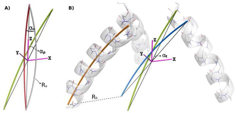
The geometric meaning of the parameters involved in the arched bundle parameterization can be best understood by considering the transformations necessary to build such a bundle. A) The tube shown in gray is the initial bent helical curve with a radius of curvature of Ra around which an α-helix is to wind. The Z-axis is the principal bundle axis and the first chain is taken to lie in the XZ-plane. αu, the arc turn angle, is the angle by which the helix arc planes of individual monomers are turned with respect to the primary axis in the eventual bundle. Thus, to dial in this parameter, the initial curve is rotated around the Z-axis by αu, resulting in the orange curve. Bundle pitch is established by rotating the new helical curve around the Y-axis by the pitch angle αp, resulting in the curve shown as a green tube. B) Bundle tilt is created by rotating the helical curve around the X-axis by the tilt angle αt, resulting in the helical curve show as a blue tube. The helical curve is translated along the X-axis by an amount equal to the bundle radius Rb and a helix is wound around the resulting curve given a particular helix starting phase φ1 (orange tube and gray helix). Other members of the bundle are either generate using ideal phase offsets of , where n is the number of chains or, alternatively, phase offsets are assigned individually for each chain after the first one.
This motif is particularly common in TM and near-TM regions of channel proteins and bacterial signaling proteins. We manually inspected all representative structures of channel proteins in the OPM database[38] and found one or several such arched bundles in all channel superfamilies and in virtually all families (see Table 1 for a list of representative structures). As with the Crick parameterization, arched bundles can be fit with their ideal counterparts rather well, in most instances producing Cα RMSD of less than 1 Å (see Table 1).
Table 1.
List of representative structure with arched bundles
| PDB ID & Region1 | N2 | Ra, Å (ε, °)3 | Rb, Å4 | αt, ° 5 | αp, ° 6 | αu, ° 7 | φeff, ° 8 | err, Å 9 | Annotation |
|---|---|---|---|---|---|---|---|---|---|
| 1NKZ, outer bundle | 9 | 93.9 (14.7) | 30.6 | −8 | 13 | −115 | 84 | 0.34 | light-harvesting complex LH2 |
| 1NKZ, inner bundle | 9 | 93.8 (11.1) | 16.9 | −1 | 4 | −150 | −106 | 0.29 | light-harvesting complex LH2 |
| 1IJD, outer bundle | 9 | 83.4 (15.5) | 30.7 | −8 | 13 | −116 | −176 | 0.36 | light-harvesting complex LH3 |
| 1IJD, inner bundle | 9 | 94.5 (10.1) | 17.4 | −1 | 5 | −136 | −13 | 0.28 | light-harvesting complex LH3 |
| 3BEH, inner bundle | 4 | 87.5 (11.9) | 11.3 | 29 | 22 | 53 | 60 | 0.37 | bacterial cyclic nucleotide-regulated channel MlotiK1 |
| 1R3J, inner bundle | 4 | 234.9 (4.9) | 10.2 | 27 | 23 | −85 | 74 | 0.36 | potassium channel KcsA |
| 1R3J, outer bundle | 4 | 51.3 (20.1) | 17.0 | −14 | 15 | 118 | −24 | 0.24 | potassium channel KcsA |
| 1S5H, outer bundle | 4 | 50.4 (20.3) | 16.9 | −14 | 16 | 118 | −26 | 0.23 | potassium channel KcsA |
| 1S5H, inner bundle | 4 | 240.7 (4.8) | 10.1 | 27 | 23 | −88 | 74 | 0.36 | potassium channel KcsA |
| 1S5H, selectivity filter bundle | 4 | 53.5 (10.4) | 13.4 | 47 | −8 | −95 | 145 | 0.18 | potassium channel KcsA |
| 3EFF, outer bundle | 4 | 96.6 (10.5) | 19.1 | −5 | 19 | 88 | −83 | 1.26 | potassium channel KcsA, full-length, closed state |
| 3EFF, inner bundle | 4 | 374.1 (2.7) | 12.0 | 27 | 22 | −13 | 74 | 0.56 | potassium channel KcsA, full-length, closed state |
| 2A79, inner bundle | 4 | 42.5 (18.2) | 13.2 | 26 | 26 | 70 | −179 | 0.38 | potassium channel Kv1.2 |
| 2A79, outer bundle | 4 | 64.2 (10.6) | 18.4 | −11 | 38 | −164 | 73 | 0.29 | potassium channel Kv1.2 |
| 2A79, selectivity filter bundle | 4 | 41.7 (13.7) | 13.8 | 49 | −8 | −57 | 150 | 0.32 | potassium channel Kv1.2 |
| 2R9R, outer bundle | 4 | 66.1 (13.6) | 17.9 | −9 | 34 | −150 | −25 | 0.23 | K+ channel Kv1.2, membrane-like environment |
| 2R9R, inner bundle | 4 | 53.6 (15.3) | 13.4 | 25 | 25 | 64 | 73 | 0.31 | K+ channel Kv1.2, membrane-like environment |
| 2R9R, selectivity filter bundle | 4 | 23.9 (24.8) | 14.1 | 51 | −9 | −38 | 136 | 0.52 | K+ channel Kv1.2, membrane-like environment |
| 1ORQ, inner bundle | 4 | 41.7 (35.0) | 8.0 | −5 | 52 | 99 | 20 | 0.81 | K+ channel KvAP |
| 2A0L, outer bundle | 4 | 70.2 (14.8) | 19.5 | −2 | 35 | −78 | −89 | 0.43 | K+ channel KvAP |
| 2A0L, inner bundle | 4 | 36.4 (34.0) | 9.1 | 9 | 47 | 105 | 36 | 0.65 | K+ channel KvAP |
| 3E86, outer bundle | 4 | 138.7 (5.9) | 19.5 | −1 | 21 | −118 | 133 | 0.21 | K+ channel, open state |
| 3E86, inner bundle | 4 | 23.3 (40.1) | 12.2 | 17 | 36 | 96 | 164 | 0.54 | K+ channel, open state |
| 3E86, selectivity filter bundle | 4 | 189.1 (2.9) | 12.9 | 45 | −14 | −118 | 161 | 0.17 | K+ channel, open state |
| 2AHY, outer bundle | 4 | 149.6 (5.3) | 19.0 | −5 | 13 | 107 | 123 | 0.24 | K+ channel, closed state |
| 2AHY, inner bundle | 4 | 99.6 (9.1) | 12.7 | 21 | 16 | 94 | 173 | 0.28 | K+ channel, closed state |
| 2AHY, selectivity filter bundle | 4 | 104.0 (5.3) | 12.9 | 44 | −17 | −84 | 166 | 0.19 | K+ channel, closed state |
| 2QKS, outer bundle | 4 | 169.7 (6.1) | 17.7 | −6 | 40 | −131 | 86 | 0.24 | Kir3.1-prokaryotic Kir channel chimera |
| 2QKS, inner bundle | 4 | 95.4 (13.4) | 10.0 | 17 | 28 | 77 | 61 | 0.26 | Kir3.1-prokaryotic Kir channel chimer |
| 1P7B, outer bundle | 4 | 396.8 (2.4) | 17.9 | −4 | 41 | −177 | −10 | 0.33 | K+ channel Kirbac1.1 |
| 1P7B, inner bundle | 4 | 115.4 (9.2) | 11.4 | 25 | 22 | 68 | 71 | 0.45 | K+ channel Kirbac1.1 |
| 1XL6, outer bundle | 4 | 237.2 (4.2) | 18.4 | −5 | 40 | −48 | 91 | 0.28 | potassium channel Kirbac3.1 |
| 1XL6, inner bundle | 4 | 96.0 (13.2) | 10.5 | 18 | 28 | 40 | 59 | 0.38 | potassium channel Kirbac3.1 |
| 2OAU, TM3 bundle | 7 | 73.7 (15.5) | 25.8 | −26 | 25 | 136 | −108 | 1.92 | mechanosensitive channel MscS, expanded state |
| 2OAU, TM2 bundle | 7 | 131.3 (7.7) | 24.5 | 32 | 19 | 64 | 158 | 2.01 | mechanosensitive channel MscS, expanded state |
| 2OAU, TM1 bundle | 7 | 116.7 (5.9) | 10.6 | 1 | 26 | 76 | 72 | 0.82 | mechanosensitive channel MscS, expanded state |
| 2VV5, TM3 bundle | 7 | 91.0 (12.8) | 27.7 | −11 | 49 | 149 | −125 | 0.34 | mechanosensitive channel MscS, open state |
| 2VV5, TM2 bundle | 7 | 122.8 (8.4) | 23.3 | 18 | 32 | 61 | 175 | 0.37 | mechanosensitive channel MscS, open state |
| 2VV5, TM1 bundle | 7 | 58.3 (11.6) | 13.4 | −8 | 6 | 109 | 87 | 0.24 | mechanosensitive channel MscS, open state |
| 3EAM, inner bundle | 5 | 194.2 (5.1) | 9.6 | −6 | −1 | 43 | −139 | 0.39 | ligand-gated ion channel, open conformation |
| 2RLF, TM bundle | 4 | 109.6 (7.9) | 7.6 | −4 | −16 | 32 | −162 | 0.35 | M2 channel TM domain, closed state |
| 3C9J, TM bundle | 4 | 662.0 (1.3) | 8.5 | −20 | −31 | 91 | 179 | 0.47 | M2 channel TM domain, open state, complex with amantadine |
| 3H9V, inner bundle | 3 | 42.8 (27.0) | 9.7 | −33 | −42 | −20 | −107 | 0.61 | ATP-gated P2X4 ion channel, the closed |
| 2O9B, GAF domain helices α8 | 2 | 121.7 (8.3) | 6.3 | 7 | −11 | −61 | −170 | 0.90 | bacteriophytochrome chromophore binding domain |
| 2O9C, GAF domain helices α8 | 2 | 113.4 (8.9) | 6.3 | 7 | −10 | −65 | −170 | 0.90 | bacteriophytochrome chromophore binding domain |
| 2O9C, GAF domain helices α4 | 2 | 38.9 (16.8) | 8.0 | −23 | 3 | 158 | 26 | 0.51 | bacteriophytochrome chromophore binding domain |
| 3E98, dimer interface helices | 2 | 37.1 (22.1) | 10.0 | 6 | −6 | −40 | −155 | 0.66 | GAF domain of unknown function |
| 3E98, dimer interface helices | 2 | 121.2 (6.0) | 6.6 | −3 | −3 | 78 | −34 | 0.30 | GAF domain of unknown function |
| 2HGV, dimer interface helices | 2 | 131.6 (5.8) | 7.0 | 3 | 4 | −3 | −77 | 0.24 | GAF domain of transcriptional repressor CodY |
| 2HGV, dimer interface helices | 2 | 58.9 (11.7) | 8.6 | −9 | −2 | −112 | −30 | 0.30 | GAF domain of transcriptional repressor CodY |
| 1IXM, dimer interface helices | 2 | 77.2 (13.5) | 5.9 | −3 | 7 | −88 | −8 | 0.36 | B. subtilis Spo0B phosphotransferase |
| 1LIH, dimer interface helices | 2 | 63.3 (17.8) | 3.9 | −1 | −9 | 154 | 155 | 0.28 | Bacterial aspartate receptor ligand-binding domain |
| 2LIG, dimer interface helices, Asp-bound form | 2 | 64.4 (17.6) | 4.0 | −1 | −8 | 157 | 150 | 0.29 | Bacterial aspartate receptor ligand-binding domain |
| 1LIH, dimer interface outer helices | 2 | 170.0 (5.8) | 10.9 | 4 | −11 | −172 | 49 | 0.19 | Bacterial aspartate receptor ligand-binding domain |
| 2LIG, dimer interface outer helices, Asp-bound form | 2 | 171.9 (5.7) | 11.1 | 4 | −9 | 180 | 49 | 0.32 | Bacterial aspartate receptor ligand-binding domain |
Supplementary Table S3 lists the regions fit within each OPM entry
Number of chains;
Arc radius and in parentheses arc incident angle;
Bundle radius;
Tilt angle;
Pitch angle;
Arc turn angle;
Effective helix phase (φ1 + αu);
Fitting Cα RMSD (Å)
Some general trends are already apparent from the limited data on arched-bundle preferred parameters. The degree of helix bending in these bundles can be rather severe, with radii of curvature as low as 23 Å and an average helix diverging by ~ 23° from its initial direction over 20 residues, the length of a typical TM segment. Such range of bending is similar to what has been observed in water soluble proteins[44, 45]. At the same time, it has been argued from physical considerations that, in general, membrane-inserted helices should be more regular than their soluble counterparts, and NMR-based mapping of torsion angles of the influenza A M2 proton channel has been used to provide experimental evidence for this[46]. The instances of significant bending we observe in arched bundles may thus be unusual, and this may be of significance in light of the functionally important regions these bundles are found in.
Although we observe a large range of bundle radii in arched bundles, even within a single oligomerization state (average standard deviation within an oligomerization state ~ 5.3 Å), mean radius, like with coiled coils, follows a roughly linear relationship with the number of chains (see Supplementary Figure S9). Arc turn angle, which characterizes the rotation of the plane of the arc relative to the bundle axis, is distributed around 90° (see Supplementary Figure S10), indicating that most often the helices bend in a direction roughly tangential to the channel pore. The sign of the pitch angle parameter (see Figure 9) indicates whether the helix crossing is left-handed or right-handed, corresponding to negative and positive pitch angles, respectively. Based on this, 18 of the analyzed bundles are left-handed and 37 right-handed (see Table 1), an interesting contrast with the coiled coil.
3. Discussion
Effective low-dimensionality descriptions of protein structure are very desirable as they simplify the task of establishing relationships between structure and function or other properties. For example, understanding biological signaling as it relates to changes in structural states of proteins has been effective in terms of gross structural rearrangements[47, 48, 49]. In structure prediction and design, low-complexity representations of structure limit the space of potential templates and can help elucidate sequence-based preferences for various structural environments[50, 51]. Simple classification schemes such as hydrophobicity scales or α-helix/β-sheet propensities represent examples of this, and so do more complex approaches such as identification of sequence motifs encoding specific geometries of secondary-structure packing [32, 51].
Another task simplified by the use of reduced structural representations is that of relating structure to designability – the size of sequence space compatible with a given structure. This is a task of great significance in protein design and particularly de novo design, where backbone templates cannot be borrowed from existing structures and one must limit oneself to targeting only templates of reasonable designability. Here we demonstrate the use of structural parameterization for describing designability, starting with the Crick parameterization of the α-helical coiled coil. We show that for over 95% of annotated coiled-coil structures, an ideal parameterized backbone can be found within 1.0 Å Cα RMSD of the native structure. In fact, we find that instead of the very large space of possible parameter value combinations, natural structures populate only very restricted areas in parameter space. For example, characteristic values of the superhelical radius grow linearly with the number of chains, and the amount of variation within each oligomerization state is around ± 1 Å (a standard deviation of ~ 0.5Å; see Supplementary Figure S3). This means that given the desired oligomerization state to be targeted in design, reasonably designable templates have superhelical radii in a narrow range. Further, within this range, certain amino acids, when occurring at core a and d positions, have well-defined preferences for certain radius values, whereas others are fairly forgiving (see Figure 5). In the latter category is Leu at the a position, the most common residue in this position of coiled coils. This makes Leu a very important amino acid for the designability of coiled coils, without which the space of designable structures would be much more restricted. Superhelical radius can also change significantly within a single coiled coil (see Supplementary Figures S5 and S4). In fact, the radius can vary by as much as 0.14 Å per residue, amounting to a contraction or expansion of 0.7 Å over a single heptad. The ability of coiled coils to adopt different local parameters can be a useful feature in design.
It is well known that amino-acid preferences at a and d are different[52] and we have now also shown that the ability of amino acids to accommodate different-sized supercoils also differs at these two positions (compare Figures 5A and B). Indeed, a and d are also non-symmetric in the sense of helical phase, which is apparent from Figure 8. On average, the Cα atom of an a position is closer to the interhelical axis than that of a d position, with the vectors connecting these atoms to the helical center offset by 17° relative to the interhelical vector (see Figure 8). The distribution of helical phases shows seven clear peaks, corresponding to the heptad repeat. Notably, these peaks are rather narrow with standard deviations ~ 8°. Interestingly, we found no correlation between the locations of these peaks and orientation, oligomerization state or axial offset. Alber and co-workers have studied the packing differences of a and d residues in different oligomerization states by comparing core structures of dimeric, trimeric and tetrameric variants of the GCN4 coiled coil[53]. The authors point out that the angle between the Cα–Cβ vector of the a/d residue, defining the “knob”, and the opposing Cα–Cα vector, defining the “hole” into which the knob packs, change in going from dimer, to trimer, to tetramer. These findings are entirely consistent with our observation of helical phase invariance with respect to oligomerization state. As helices move around the superhelical circle to make room for more monomers, the α-helical phase of each monomer (defined with respect to the interfacial axis) stays roughly unchanged, whereas the orientation of the Cα–Cα vector defining the “hole” does change with respect to partnering helices, giving precisely the trend observed by Alber and co-workers (see Supplementary Figure S11).
We found that the axial alignment at the helix-helix interface is very restricted in natural backbones, but in different ways for parallel and anti-parallel helix pairs. As can be seen from the distribution of parameter ΔZaa′ in Figure 7, parallel coiled-coil pairings tend to align helical turns of adjacent helices at the same level along the interface axis, corresponding to ΔZaa′ of zero, whereas in anti-parallel orientations, helical turns tend to interdigitate at the interface. Further, anti-parallel coiled coils interdigitate with considerable asymmetry, with a positions preferring to pack between the upstream d′ (e.g. in the C→N direction of the first helix) and the downstream a′ (N→C direction of first helix; see Figures 7 and 10 and Supplementary Figure S8).
Figure 10. Structural reasoning behind different ΔZoff preferences between parallel and anti-parallel alignments.

A) and B) illustrate parallel and anti-parallel dimeric coiled coils, respectively (images generated with coiled coils taken from PDB entries 2ZTA and 2NOV, respectively). Cylinders represent local orientation of helices, black spheres show Cα atoms and gray spheres depict Cβ atoms. Only a and d positions are shown. Given the direction of Cα-Cβ vectors on opposite chains, in anti-parallel alignments, a potential steric repulsion between a and a′ residues in adjacent layers (depicted with a dotted line) pushes the preference of ΔZoff away from zero.
The origin of this difference can be rationalized by considering the chirality of the Cα atom and the fact that in an α-helix, the Cα-Cβ vector has a positive component in the C→N direction. Adjacent a and d positions of a coiled coil are on opposite sides of the interface, separated along the interfacial axis by ~ 4.5 Å from a to the next d and ~ 6.0 Å from d to the next a. In a parallel alignment, where the Cα-Cβ vectors of both chains point in the same direction along the helix, this makes it possible for the a and d positions of opposite chains to situate across from one another, forming a-a′ and d-d′ interactions (see figure 10A). In an anti-parallel alignment, however, because Cα-Cβ vectors of opposite chains point in opposite directions, potential steric interactions arise between core residues of opposite chains located on the same side of the interface (i.e. a - a′ and d - d′), as shown figure 10B. Indeed, it is easy to see that unless core residues are small, an on-level alignment (e.g. ΔZoff = 0) will not be preferred, but rather, an a residue of one chain will pack between adjacent d′ and a′ residues of the other chain and vice versa. The detailed alignment, of course, depends on the exact sequence, but the overall trends of ΔZoff are consistent with these simple geometric considerations. These findings are also consistent with the description of the anti-parallel Alacoil by the Richardsons and co-workers[54]. By analyzing seven unrelated proteins, the authors identified an anti-parallel dimeric coiled-coil motif, the Alacoil, in which small residues at a and d positions allow for a very close approach of helices. In addition to the on-level helical alignment akin to the one seen in parallel coiled coils, the authors observed another type of axial offset, corresponding precisely to the interdigitated alignment described above. In the case of Alacoil, geometric preferences can be understood in terms of the close helical packing and small residues at a and d[54]. However, we observed the median superhelical radius for anti-parallel dimers to be only marginally smaller than that for parallel dimers (4.82 Å and 4.92 Å, respectively), with corresponding distributions overlapping very significantly (see Figure 4B). On the other hand, the difference between distributions of helical offsets for parallel and anti-parallel alignments is striking, indicating that closer helical approach alone cannot account for this effect. The difference between axial alignment of parallel and anti-parallel coiled coils is also in agreement with recent results by Gellman and co-workers, demonstrating significant thermodynamic coupling between residues at the a position of one chain and the a′ position of the opposite chain in anti-parallel dimeric coiled coils[55].
All of the analyzed coiled-coil parameters are strongly restricted, reflecting a well-defined and narrow space of designable structures. In fact, based on analyzing the degree of restriction in parameters R0, α, ΔZaa′, and φ1, we estimate that the space of designable structures is at least 160–200 fold reduced relative to the space of physically reasonable backbones. In the context of de novo design this means that a template selected purely on the basis of geometric feasibility is very unlikely to have significant designability. This is likely to be the case for protein structures in general, illustrating the need for effective low-dimensionality parameterization schemes in other systems.
To begin addressing this need, we developed a general method for parameterizing arbitrary helical structures. Further, we used it to characterize an α-helical motif we found to be common in inner linings of channel and transporter proteins, the surrounding secondary bundles as well as in dimerization interfaces of bacterial signaling proteins. These bundles consist of helices that are bent into nearly perfectly circular arcs. Using our generalized method, we describe these structures parametrically with a handful of simple geometric variables (see Figure 9 and Table 1). We find that the degree of helix curvature in these bundles can be rather significant, with radii of curvature as low as 23 Å (for comparison, a typical coiled coil has a radius of curvature of ~ 100 Å). In their classical work on the geometry of helices in proteins, Barlow and Thornton found similarly curved helices in water soluble proteins[44]. In fact, among all helices characterized as curved in their work, the lowest and the median radii of curvature were 29 and 62 Å, respectively, whereas for our set of bundles these are 23 and 64 Å, respectively (for the latter, we defined as curved helices with a radius of curvature below 100 Å). Barlow and Thornton showed that the center of helix curvature of regularly curved (amphipathic) α-helices tended to lie on the hydrophobic side of the helix, due to backbone hydrogen bonds being on average shorter in hydrophobic environments and longer in a solvent-exposed environments. Is this also the reason for the curvature we observe in arched bundles? In some instances this is clearly the case, as there are crystallographically-resolved water molecules that form hydrogen bonds with the backbone amide hydrogen and carbonyl oxygen atoms, allowing one side of the helix to stretch out and creating a bend. For example, this can be seen in the 1.5 Å resolution structure of an NaK channel from Bacillus cereus[56] (PDB code 3E86, see Supplementary Figure S12A). However, in other cases, such waters are not explicitly seen, and a single structural reason for the presence of the bend is difficult to identify (e.g. in the structure of the voltage-dependent potassium channel KvAP[57], PDB code 1ORQ, see Supplementary Figure S12B). One might expect that helices in channel-forming bundles may curve radially from the channel central axis, as the extent of solvent exposure may be quite different for the pore-facing side of the helix and the membrane/protein-facing side. However, the distribution of arc turn angles from our parameterization (see Figure 9) demonstrates that most often bending occurs in the plane approximately tangential to the channel pore (see Supplementary Figure S10). Likely, membrane helical curvature arises as a consequence of a combination of effects, reconciling different extents of solvent exposure (with potentially specific water molecules present in the membrane), amino-acid bilayer solvation preferences, and the energetic preference for a particular crossing angle imposed by the full protein structure.
Backbone-parameterized models of protein structure can be a very powerful approach for describing the diversity within a family of structures and relating it to designability. We have used this principle to demonstrate that the space of naturally designable coiled coils is restricted at least 160–200 fold relative to the space of geometrically reasonable structures. We have also provided a general framework for parameterization of arbitrary helical structures and have used it to parametrically describe pore-forming bundles of TM channel proteins and subunit interfacial bundles of bacterial signaling proteins.
Rearrangements along coordinates of a well-chosen parameterization may be functionally relevant. Structurally well populated modes of helix-helix interaction occur in specific discrete crossing geometries[32], such that tilting and pitching of helices with respect to each other in a complex bundle would appear to be a convenient way of establishing a discrete set of local minima. Arching of helices also appears to be well suited for establishing alternate states and transferring information. Because arching corresponds to low-frequency bending modes of the α-helix, differently bent conformations would be expected to intercovert at a low frequency in the background, while the presence of various conditions, such as signaling ligands, could stabilize some conformations relative to others.
4. Materials and Methods
4.1. Database
Coiled-coil structures were obtained from the CC+ database[39] as of August 20th, 2009. This database was generated by Woolfson and colleagues using the structure-based coiled coil recognition program SOCKET[41] applied exhaustively to the entire Protein Data Bank. Our initial set of 3,902 structures was obtained by searching CC+ for all entries longer than 11 amino acids using the web-based dynamic search interface. For later analysis, a sequence redundancy filter of 50% was added in the CC+ search interface, which resulted in 868 structures returned by CC+. Sequence redundancy between two coiled coils in CC+ is considered only for structures of identical topology (e.g. the same orientation and oligomerization state). It is calculated as the average percent identity between matching chains of the two complexes, where each chain in one complex is matched up against its closest in sequence counterpart in the other complex (see reference [39] for details). Additionally, five structures of right-handed coiled coils were manually added to the database as a result of distance map-based searches of the PDB for such topologies (see below for a description of the search method). The resulting database contained structures ranging from 12 to 148 residues per chain (or 24 to 393 residues per structure), although shorter structures were more common (see Supplementary Figure S1). Supplementary Table S2 summarizes the distribution of structures among different topologies within the final dataset.
4.2. Crick Parameterization Equations
The basic Crick equations describing Cartesian coordinates of a backbone atom type in the α-helix of a coiled coil, are as follows (assuming the interfacial axis is aligned with the Z-axis)[8]:
where R0, ω0, and φ0 are the superhelical radius, frequency, and phase, respectively, R1, ω1, and φ1 are the helical radius, frequency, and phase, respectively, α is the pitch angle, and t is residue index. In order to accommodate the ability of helices to shift with respect to one another along the Z-axis, these equations were modified to include an additional degree of freedom Δz. Thus, the equations used in this study were:
| (2) |
| (3) |
| (4) |
where is . This last adjustment was made to decouple axial shift from superhelical phase. Thus, Δz is the helical Z-shift produced by sliding a chain along the superhelical curve. During the fitting procedure, each chain, except the first one, was assigned its own values of φ0 and Δz, relative the first chain, and each chain had its own φ1.
An issue with Δz is that it describes the axial offset between chain ends rather than the axial alignment of the interface. To address this, we created two additional derived parameter, ΔZoff and ΔZaa′. To define ΔZoff, inward facing points on each helix are identified (see Figure 1), which are the points along the parametric helical curve that have a phase of π (i.e. they point directly into the interface). The smallest Z-offset between these points on the two chains considered is defined as ΔZoff between the two chains, with sign being positive if the second chain is shifted in the N→C direction of the first one, and negative for the opposite shift direction. The sign is meaningful for for anti-parallel helix pairings or for parallel, heterodimeric pairings. Given this definition, the value of ΔZoff can range between plus and minus a quarter of a helical pitch, or , where ω1 and d are the helical frequency and rise per residue, respectively. For a typical helix, this corresponds to the range of [−2.6, 2.6] Å.
ΔZaa′ is defined in a similar manner, except instead of points with a helical phase of π, Cα atoms of a positions on either chain are used as reference points (heptad assignment is made upon the completion of the fitting procedure, based on best fit helical phases, using the canonical values discussed in the Results section). Thus, ΔZaa′ can vary between plus and minus half a helical pitch, roughly , or [−5.3, 5.3] Å for a typical coiled coil.
4.3. Fitting Procedure
The program to fit Crick parameters given a structure, called CCCP – Coiled-Coil Crick Parameterization, was written in Matlab (see http://www.mathworks.com/), using basic functionality and some functions from the Optimization Toolbox. The code is compatible with GNU Octave[58] (see http://www.octave.org/), with no significant difference in performance, and the web-based version of CCCP uses Octave.
The entire fitting procedure can be broken down into several steps. First, given the input structure file, the number of chains is determined and Cα coordinates are extracted. For each chain (except the first one), its orientation with respect to the first chain is determined by testing the sign of the dot product between vectors connecting the first and the last atoms of the two chains. Next, the order of chains, in a clockwise direction when looking down the positive Z direction, is determined. This is important for oligomeric states above dimer so that chains of the generated ideal structures are superimposed on their corresponding chains in the native structure. To do this, Cα center of mass of each chain is identified (e.g. points through for n chains) and the center of the bundle is taken to be the average of these points (e.g. point ). Chain order is then determined by measuring the angles [ ] for each k between 1 and n. Angles are defined in a clock-wise direction, with respect to the positive Z direction, and mapped onto the range between 0 and 2π (clockwise versus counterclockwise is determined by testing whether the cross product between vectors and is aligned with the positive Z direction (i.e. whether is positive or negative). Thus, sorting the angles in ascending order produces the order of chains in the clockwise direction.
Next, parameter optimization begins. The objective function to minimize is the RMSD between atoms of the parameterized structure and the input structure (optimal superposition was implemented via the SVD method by Kabsch et al.[59] as described by Coutsias et al.[60]). Basic parameters R0, R1, ω0, ω1, α, and φ1 are always varied in optimization, and CCCP has a variety of options to limit additional variables. For example, one may wish to assume rotational symmetry about the supercoil axis and set individual chain superhelix phase offsets to , for chain i of an n-mer; alternatively, this parameter may be individually variable for each chain. Similarly, one may wish to force all chains to have the same starting phase φ1 or have this parameter float between different chains. In all of the fits performed in this paper, no assumptions of symmetry were made. Thus, in addition to the six basic parameters, each chain was also assigned its own value of φ1 and all chains after the first one were assigned values for φ0 and Δz relative to the first chain. The optimization proceeded in a loop until convergence (i.e. RMSD change per iteration was less than 10e-5 Å). In each iteration of the loop, first each parameter (except R1 and ω1) was optimized individually using the BFGS Quasi-Newton method with a cubic line search procedure, implemented in function fminunc of Matlab. The order in which individual parameters are optimized was found to be important for optimal convergence and the order used was Δz for each chain, φ0 for each chain, φ1 for each chain, R0, ω0, and α. This was followed by multi-variable optimization of all parameters at once (including R1 and ω1) first with non-linear least-squares (function lsqnonlin in Matlab) and then with BFGS Quasi-Newton method with a cubic line search procedure (fminunc in Matlab).
In cases of short dimeric coiled coils with minimal superhelical curvature, multiple combinations of superhelical radius and superhelical phase offset values can be equally fitting in terms of RMSD (for a visual example, see Supplementary Figure S13). To avoid this problem of under-determinedness, φ0 was constrained to be around π for dimers. During optimization (and not for the purpose of reporting the final RMSD), the objective function value for dimers was incremented by , where L was chain length. That is, the score was penalized by 0.02 Å for a deviation of from the optimal value of π for every three heptads. φ0 was not simply fixed at π because in some instances the most appropriate value of phase offset may truly be different from π (e.g. when the dimer looks more like two chains of a tetramer as shown in Supplementary Figure S13) and φ0 should be allowed to adjust for that, provided enough improvement in RMSD results. This small penalty resulted in the overwhelming majority of dimers to have a φ0 of nearly π.
Once an optimal Cα trace is obtained, the final step is to build the remaining backbone atoms. These were built using a table of internal coordinates (dihedral angles, angles and distances) of N and C backbone atoms with respect to known Cα atoms. These internal coordinates and their average values, extracted from the structure of GCN4 (PDB code 2ZTA), are show in Supplementary Table S1. Backbone oxygen and hydrogen atoms were then placed using standard bond length, angle and dihedral angle values from CHARMM[61]. This fast and simple approach proved robust and backbones thus produced were generally not found to be in need of further adjustment. However, CCCP (including the web-based version) can optionally subject the produced backbone to short molecular-mechanics minimization.
4.4. Local R0 as a function of core composition
For all dimers longer than three heptads, local values of R0 were calculated by CCCP fitting of two-heptad segments scanned across each structure. Superhelical radius auto-correlation length was defined as the lag, in terms of the number of residues, at which the auto-correlation function crossed zero. Two simple models for the dependence of R0 on the a and d-position amino-acid composition were considered. The relationship may be linear, whereby each residue contributes a certain fixed context-independent component, whether negative or positive, to the final R0, relative to some average reference value. Or it may be that each residue has its own radius preference and the residues with the largest preference dictate the eventual local R0. To simplify interpretation and to limit the number of parameters, we focused on parallel dimers. In both cases, there are 40 parameters (for 20 naturally occurring amino acids at either the a or d position), and the two models can be written as:
| (5) |
| (6) |
where a⃗ and d⃗ are the indices of a and d positions in the considered window, respectively, and are the i-th amino acids in either of the two chains of the dimer, and wa and wd are amino-acid dependent weights at a and d positions, respectively. In both models, wh (aai) corresponds to the context-independent contribution of amino acid aai at heptad position h (either a or d) to the final radius. Thus, the contribution of an a-a′ layer (prime designates the opposite chain) is the sum of contributions of the two amino acids forming the layer or , and the contribution of a d-d′ layer is . What differentiates the models is that in the first one, the final radius preference is dictated by the average of the layer preferences, whereas in the second one, the layer with the largest radius preference dominates. These models were fit to local R0 data described above, with results shown in Supplementary Figures S6.
4.5. Quantifying the Degree of Restriction of Natural Coiled-coil Space
For a given coiled-coil parameter x, for which we observe values ranging from xmin to xmax in natural coiled coils, we compare its observed distribution with a uniform random distribution over the range xmin to xmax. To this end, we create a histogram of the observed distribution by binning values into n bins and calculate the entropy of this histogram as , where Nobs is the total number of data points and Ni is the number of x values within bin i. Next, we compose a uniform random distribution of Nobs values over n bins, by apportioning points into all bins and an additional point into bins. The entropy of this distribution thus becomes . The quantity ΔS = S ref (x, n) − S (x, n) is then a measure of information content within the naturally observed distribution of x. If we interpret entropy in the statistical-mechanical sense, then eΔS is the ratio between the effective “number of states” in the uniform distribution and the native distribution, thereby providing us with a reasonable estimate of the degree of restriction of the natural space.
Given a limited amount of data, the number of bins n has an impact on the calculated information content. With very few bins, the natural and uniform distributions converge as everything eventually collapses to one bin. The same happens when the number of bins is too large, as eventually all bins, in both the natural and uniform distributions, either have one observation or none. To find a value of n that optimally captures the amount of information present in the observed dataset, we chose the value that maximizes the quality ΔS.
4.6. Generalized Parameterization
An α-helix is described by a simple parametric set of equations for a left-handed screw:
| (7) |
where t is the parameter (residue index) and d is rise per residue (discussed in the Results). The Crick parameterization describes what happens to this screw when it, in turn, is twisted into a larger screw, the superhelix. To address a general version of this problem, suppose that the α-helix is bent into an arbitrary shape describe by a generic parametric set of equations:
where subscript 0 designates coordinates of the superstructure and s is the new superstructure parameter. For convenience, let us consider the locations of Cα atoms, although identical reasoning can be applied for any backbone atom type. In an ideal Z-aligned helix, the Z coordinates of successive Cα atoms change in increments of d, such that a local coordinate frame can be defined for the i-th Cα atom with an origin [0, 0, z(ti)] and axes pointing in the same direction as the laboratory frame in which equation 7 is defined. Correspondingly, when the helix winds around the parametric curve, these local origins will translate onto points on the new curved axis, each corresponding to a particular parameter value si. For every residue in the final structure, the superstructure ought to sweep out an arc length equal to d, to ensure that the helix is locally neither stretched nor compressed. Thus, for going from residue i to residue i + 1 we must satisfy:
| (8) |
where si and si+1 are the values of s corresponding to residue i and i + 1, respectively. For the case of a superhelix (and thus fx(s) = R0 cos(ω0 s + φ0), fy(s) = R0 sin(ω0 s + φ0), and ) we get simply that or that , meaning that s values along the superhelix, corresponding to Cα atoms, occur at regular intervals. This does not, however, need to be the case in general. For more complicated shapes (e.g. a coiled coil of changing radius), s values from one residue to the next will change differently in different parts of the curve (e.g. more slowly the larger the radius gets).
For many parametric shapes the integral in equation 8 can be analytically solved, in which case values of si are easily obtainable. But even in cases where the integral does not exist in closed form, simple numerical integration methods can be applied to solve equation 8 efficiently. In the latter case, values of si are built up starting from the known s1, which defines the starting position along the parametric curve, and each time obtaining the value of sk+1 that validates equation 8 given the known sk. Finding all si values identifies the origins of local coordinate frames associated with each residue in the final structure (e.g. [fx(si); fy(si); fz(si)]) and we must now define the axes. Naturally, the local Z axis is defined in the direction of the gradient of the parametric curve at si, providing a smooth transition from a straight to a curved helix, whereas the X axis is defined in the direction opposite to the curvature vector of the parametric curve at si:
where primes designate derivatives with respect to s and gx, gy, and gz are the components of the normalized gradient vector g⃗ = [gx; gy; gz]. By analogy with the coiled coil, this ensures that the X axis points away from the center of rotation of the local stretch of the parametric curve. And in the case of a superhelical parametric curve, this definition recapitulates exactly that by Crick[8].
Once the local coordinate frame associated with each residue in the final structure is defined, and given the original local coordinate frame for each residue in the straight helix, two rotations and a translation are applied to transform each residue from the straight helix into its position within the curved helix. Therefore, the generalized helical parameterization framework takes on the form of a numerical procedure, rather than a simple formula, as with the coiled coil, since it is not guaranteed that the integral in equation 8 is analytically solvable. If it is, however, a formula can be derived as well, as all terms within the above rotation and translation matrices become analytical. Matlab (or Octave) code implementing the generalized helix bending parameterization is available upon request.
We applied this framework to generate a parameterization of arched bundles. As shown in Figure 9, individual helices were modeled as being shaped into perfectly circular arcs of radius Ra. The superstructure parametric equations, therefore, were fx(s) = Ra cos(ω0 s), fy(s) = 0, and fz(s) = Ra sin(ω0 s), with parameter s varying symmetrically around 0 (e.g. from some −s0 to +s0). This corresponds to a circular arc in the XZ plane, symmetrical about the X axis (see Figure 9A). Solving equation 8 we get , so for simplicity ω0 was set to (note, this is an arbitrary choice) so that values of s could be varied between and in increments of 1 (L is the number of residues in the chain). The normalized gradient of our superstructure curve is simply (since ω0 is positive here), and the normalized curvature vector is c⃗ = [− cos(ω0 s); 0; − sin(ω0 s)]. Thus, the rotation and translation matrices for superimposing the local coordinate frame in the ideal helix and the curved superstructure are trivial to find, and the final equations for a helix bent around a circular arc are:
| (9) |
where t varies from 0 to L − 1 (the second term in x (t) simply moves the ends of the arc so that they lie on the Z-axis, as shown in Figure 9A by the gray curve). Once the curved helix is generated, it is rotated about the laboratory Z axis by the arc turn angle αu, then the laboratory Y axis by the tilt angle αt and then the laboratory X axis by the pitch angle αp (see Figure 9). Finally, the helix is translated along the X axis by the bundle radius Rb. In our arched-bundle parameterization, we assumed that individual chains are spaced equally around the bundle, so upon generating one helix, the rest are generated with rotations about the Z axis in increments of , where n is the number of chains in the bundle.
Table 1 reports parameter values that best fit to a set of representative structures as well as the Cα RMSD of the fits. Note that for convenience of comparing parameters between different structural states, instead of helical phase (variable φ1 in equation 7), Table 1 reports the effective phase that takes into account the arc turn angle (i.e. the actual value reported is φeff = φ1 + αu). This allows phase to be reflective solely of the angular position of the first residue in the chain with respect to the interfacial axis, allowing for an independent interpretation of this parameter. Table 1 also reports an additional calculated parameter – the arc incidence angle, which measures the angle of the tangent to the arc at the initial point and the line connecting arc ends. For a straight helix this angle is zero, for a semicircle it is 90°.
4.7. Distance map-based search for right-handed coiled coils
To search for additional examples of right-handed coiled coils in the PDB, we employed a distance map-based search method. Full details of the method are to be published elsewhere, but a short description is provided here. A distance map is an n-by-n matrix of Cα to Cα distances within a protein, where n is the number of residues in the protein[62]. We first pre-computed such distance maps for all proteins in the PDB, storing them in a sparse format such that distances above 25 Å where not considered. Next, we used all of the right-handed coiled coils found in the CC+ database as search queries. For each query protein, a distance map corresponding to two helices, two heptads each, was generated. These query maps were then compared to the pre-computed distance maps, looking for optimal agreement between the query map and a sub-map of a potential matching protein, in the least-squares sense. The search was performed taking into account that the two helices will not be contiguous in sequence within the matching structure, so a linker of arbitrary length was allowed to locate between the two helices of the query map.
Supplementary Material
Acknowledgments
We would like to thank Dr. Cinque S. Soto for stimulating discussions and careful reading of the manuscript. Work in this paper was supported by NIH grants 1F32GM084631-01A1 and 5F32GM084631-02 to GG.
Footnotes
Publisher's Disclaimer: This is a PDF file of an unedited manuscript that has been accepted for publication. As a service to our customers we are providing this early version of the manuscript. The manuscript will undergo copyediting, typesetting, and review of the resulting proof before it is published in its final citable form. Please note that during the production process errors may be discovered which could affect the content, and all legal disclaimers that apply to the journal pertain.
References
- 1.Li H, Helling R, Tang C, Wingreen N. Emergence of preferred structures in a simple model of protein folding. Science. 1996;273:666–669. doi: 10.1126/science.273.5275.666. [DOI] [PubMed] [Google Scholar]
- 2.Wingreen NS, Li H, Tang C. Designability and thermal stability of protein structures. Polymer. 2004;45:699–705. [Google Scholar]
- 3.Helling R, Li H, Melin R, Miller J, Wingreen N, Zeng C, Tang C. The designability of protein structures. J Mol Graph Model. 2001;19:157–167. doi: 10.1016/s1093-3263(00)00137-6. [DOI] [PubMed] [Google Scholar]
- 4.England JL, Shakhnovich BE, Shakhnovich EI. Natural selection of more designable folds: a mechanism for thermophilic adaptation. Proc Natl Acad Sci USA. 2003;100:8727–8731. doi: 10.1073/pnas.1530713100. [DOI] [PMC free article] [PubMed] [Google Scholar]
- 5.Govindarajan S, Goldstein RA. Why are some proteins structures so common? Proc Natl Acad Sci USA. 1996;93:3341–3345. doi: 10.1073/pnas.93.8.3341. [DOI] [PMC free article] [PubMed] [Google Scholar]
- 6.Koehl P, Levitt M. Protein topology and stability define the space of allowed sequences. Proc Natl Acad Sci USA. 2002;99:1280–1285. doi: 10.1073/pnas.032405199. [DOI] [PMC free article] [PubMed] [Google Scholar]
- 7.Kuhlman B, Baker D. Native protein sequences are close to optimal for their structures. Proc Natl Acad Sci USA. 2000;97:10383–10388. doi: 10.1073/pnas.97.19.10383. [DOI] [PMC free article] [PubMed] [Google Scholar]
- 8.Crick FH. The fourier transform of a coiled coil. Acta Cryst. 1953;6:685–689. [Google Scholar]
- 9.Harbury PB, Tidor B, Kim PS. Repacking protein cores with backbone freedom: structure prediction for coiled coils. Proc Natl Acad Sci USA. 1995;92:8408–8412. doi: 10.1073/pnas.92.18.8408. [DOI] [PMC free article] [PubMed] [Google Scholar]
- 10.Murzin AG, Lesk AM, Chothia C. Principles determining the structure of β-sheet barrels in proteins. I. A theoretical analysis. J Mol Biol. 1994;236:1369–1381. doi: 10.1016/0022-2836(94)90064-7. [DOI] [PubMed] [Google Scholar]
- 11.Murzin AG, Lesk AM, Chothia C. Principles determining the structure of β-sheet barrels in proteins. II. The observed structures. J Mol Biol. 1994;236:1382–1400. doi: 10.1016/0022-2836(94)90065-5. [DOI] [PubMed] [Google Scholar]
- 12.Rainey JK, Goh MC. A statistically derived parameterization for the collagen triple-helix. Protein Science. 2002;11:2748–2754. doi: 10.1110/ps.0218502. [DOI] [PMC free article] [PubMed] [Google Scholar]
- 13.Lombardi A, Summa CM, Geremia S, Randaccio L, Pavone V, DeGrado WF. Inaugural article: retrostructural analysis of metalloproteins: application to the design of a minimal model for diiron proteins. Proc Natl Acad Sci USA. 2000;97:6298–6305. doi: 10.1073/pnas.97.12.6298. [DOI] [PMC free article] [PubMed] [Google Scholar]
- 14.Goldberg SD, Soto CS, Waldburger CD, DeGrado WF. Determination of the physiological dimer interface of the phoq sensor domain. J Mol Biol. 2008;379:656–665. doi: 10.1016/j.jmb.2008.04.023. [DOI] [PMC free article] [PubMed] [Google Scholar]
- 15.Metcalf DG, Law PB, DeGrado WF. Mutagenesis data in the automated prediction of transmembrane helix dimers. Proteins. 2007;67:375384. doi: 10.1002/prot.21265. [DOI] [PubMed] [Google Scholar]
- 16.North B, Summa CM, Ghirlanda G, DeGrado WF. D(n)-symmetrical tertiary templates for the design of tubular proteins. J Mol Biol. 2001;311:1081–1090. doi: 10.1006/jmbi.2001.4900. [DOI] [PubMed] [Google Scholar]
- 17.Havranek JJ, Harbury PB. Automated design of specificity in molecular recognition. Nat Struct Biol. 2003;10(1):45–52. doi: 10.1038/nsb877. [DOI] [PubMed] [Google Scholar]
- 18.Harbury PB, Plecs JJ, Tidor B, Alber T, Kim PS. High-resolution protein design with backbone freedom. Science. 1998;282(5393):1462–1467. doi: 10.1126/science.282.5393.1462. [DOI] [PubMed] [Google Scholar]
- 19.Grigoryan G, Reinke AW, Keating AE. Design of protein-interaction specificity gives selective bzip-binding peptides. Nature. 2009;458(7240):859–864. doi: 10.1038/nature07885. [DOI] [PMC free article] [PubMed] [Google Scholar]
- 20.Offredi F, Dubail F, Kischel P, Sarinski K, Stern AS, de Weerdt CV, Hoch JC, Prosperi C, Franois JM, Mayo SL, Martial JA. De novo backbone and sequence design of an idealized α/β-barrel protein: Evidence of stable tertiary structure. Journal of Molecular Biology. 2003;325(1):163–174. doi: 10.1016/S0022-2836(02)01206-8. [DOI] [PubMed] [Google Scholar]
- 21.Keating AE, Malashkevich VN, Tidor B, Kim PS. Side-chain repacking calculations for predicting structures and stabilities of heterodimeric coiled coils. Proceedings of the National Academy of Sciences of the United States of America. 2001;98(26):14825–14830. doi: 10.1073/pnas.261563398. arXiv: http://www.pnas.org/content/98/26/14825.full.pdf+html. [DOI] [PMC free article] [PubMed]
- 22.Grigoryan G, Keating AE. Structure-based prediction of bzip partnering specificity. J Mol Biol. 2006;355:1125–1142. doi: 10.1016/j.jmb.2005.11.036. [DOI] [PubMed] [Google Scholar]
- 23.Apgar JR, Gutwin KN, Keating AE. Predicting helix orientation for coiled-coil dimers. Proteins. 2008;72:1048–1065. doi: 10.1002/prot.22118. [DOI] [PMC free article] [PubMed] [Google Scholar]
- 24.Valavanis IK, Bagos PG, Emiris IZ. β-barrel transmembrane proteins: Geometric modelling, detection of transmembrane region, and structural properties. Computational Biology and Chemistry. 2006;30(6):416–424. doi: 10.1016/j.compbiolchem.2006.09.001. [DOI] [PubMed] [Google Scholar]
- 25.Furini S, Domene C, Rossi M, Tartagni M, Cavalcanti S. Model-based prediction of the [alpha]-hemolysin structure in the hexameric state. Biophysical Journal. 2008;95(5):2265–2274. doi: 10.1529/biophysj.107.127019. [DOI] [PMC free article] [PubMed] [Google Scholar]
- 26.Howard RJ, Clark KA, Holton JM, DLM Structural insight into KCNQ (Kv7) channel assembly and channelopathy. Neuron. (53) 2007;(5):663–675. doi: 10.1016/j.neuron.2007.02.010. [DOI] [PMC free article] [PubMed] [Google Scholar]
- 27.Zou J, Saven JG. Statistical theory of combinatorial libraries of folding proteins: energetic discrimination of a target structure. J Mol Biol. 2000;296:281–294. doi: 10.1006/jmbi.1999.3426. [DOI] [PubMed] [Google Scholar]
- 28.Wolynes PG. Symmetry and the energy landscapes of biomolecules. Proc Natl Acad Sci USA. 1996;93:14249–14255. doi: 10.1073/pnas.93.25.14249. [DOI] [PMC free article] [PubMed] [Google Scholar]
- 29.North BH. PhD dissertation. University of Pennsylvania; 2006. Application of the Crick parameterization to de novo protein design. [Google Scholar]
- 30.Offer G, Hicks MR, Woolfson DN. Generalized Crick equations for modeling noncanonical coiled coils. J Struct Biol. 2002;137:41–53. doi: 10.1006/jsbi.2002.4448. [DOI] [PubMed] [Google Scholar]
- 31.Summa CM, Lombardi A, Lewis M, DeGrado WF. Tertiary templates for the design of diiron proteins. Curr Opin Struct Biol. 1999;9:500–508. doi: 10.1016/S0959-440X(99)80071-2. [DOI] [PubMed] [Google Scholar]
- 32.Walters RF, DeGrado WF. Helix-packing motifs in membrane proteins. Proc Natl Acad Sci USA. 2006;103:13658–13663. doi: 10.1073/pnas.0605878103. [DOI] [PMC free article] [PubMed] [Google Scholar]
- 33.Engel DE, DeGrado WF. Alpha-alpha linking motifs and interhelical orientations. Proteins. 2005;61:325–337. doi: 10.1002/prot.20522. [DOI] [PubMed] [Google Scholar]
- 34.Murzin AG, Finkelstein AV. General architecture of the alpha-helical globule. J Mol Biol. 1988;204:749–769. doi: 10.1016/0022-2836(88)90366-x. [DOI] [PubMed] [Google Scholar]
- 35.Bowie JU. Helix packing angle preferences. Nat Struct Biol. 1997;4:915–917. doi: 10.1038/nsb1197-915. [DOI] [PubMed] [Google Scholar]
- 36.Walther D, Eisenhaber F, Argos P. Principles of helix-helix packing in proteins: the helical lattice superposition model. J Mol Biol. 1996;255:536–553. doi: 10.1006/jmbi.1996.0044. [DOI] [PubMed] [Google Scholar]
- 37.Zhou HX, McCammon JA. The gates of ion channels and enzymes. Trends Biochem Sci. doi: 10.1016/j.tibs.2009.10.007. [DOI] [PMC free article] [PubMed] [Google Scholar]
- 38.Lomize MA, Lomize AL, Pogozheva ID, Mosberg HI. OPM: orientations of proteins in membranes database. Bioinformatics. 2006;22:623–625. doi: 10.1093/bioinformatics/btk023. [DOI] [PubMed] [Google Scholar]
- 39.Testa OD, Moutevelis E, Woolfson DN. CC+: a relational database of coiled-coil structures. Nucleic Acids Res. 2009;37(database issue):D315–D322. doi: 10.1093/nar/gkn675. [DOI] [PMC free article] [PubMed] [Google Scholar]
- 40.Sales M, Plecs JJ, Holton JM, Alber T. Structure of a designed, right-handed coiled-coil tetramer containing all biological amino acids. Protein Sci. 2007;16(10):2224–2232. doi: 10.1110/ps.062702907. [DOI] [PMC free article] [PubMed] [Google Scholar]
- 41.Walshaw J, Woolfson DN. Socket: a program for identifying and analysing coiled-coil motifs within protein structures. Journal of molecular biology. 2001;307(5):1427–1450. doi: 10.1006/jmbi.2001.4545. [DOI] [PubMed] [Google Scholar]
- 42.Stetefeld J, Jenny M, Schulthess T, Landwehr R, Engel J, Kammerer RA. Crystal structure of a naturally occurring parallel right-handed coiled coil tetramer. Nature. 2000;7(9):772–776. doi: 10.1038/79006. [DOI] [PubMed] [Google Scholar]
- 43.O’Shea EK, Klemm JD, Kim PS, Alber T. X-ray structure of the GCN4 leucine zipper, a two-stranded, parallel coiled coil. Science. 1991;254(5031):539–544. doi: 10.1126/science.1948029. [DOI] [PubMed] [Google Scholar]
- 44.Barlow DJ, Thornton JM. Helix geometry in proteins. J Mol Biol. 1988;201:601–619. doi: 10.1016/0022-2836(88)90641-9. [DOI] [PubMed] [Google Scholar]
- 45.Kumar S, Bansal M. Geometrical and sequence characteristics of alpha-helices in globular proteins. Biophys J. 1998;75:1935–1944. doi: 10.1016/S0006-3495(98)77634-9. [DOI] [PMC free article] [PubMed] [Google Scholar]
- 46.Page RC, Kim S, Cross TA. Transmembrane helix uniformity examined by spectral mapping of torsion angles. Structure. 2008;16:787–797. doi: 10.1016/j.str.2008.02.018. [DOI] [PMC free article] [PubMed] [Google Scholar]
- 47.Grottesi A, Sands ZA, Sansom MSP. Potassium channels: Complete and undistorted. Current Biology. 2005;15(18):R771–R774. doi: 10.1016/j.cub.2005.08.054. [DOI] [PubMed] [Google Scholar]
- 48.Casino P, Rubio V, Marina A. Structural insight into partner specificity and phosphoryl transfer in two-component signal transduction. Cell. 2009;139:325–336. doi: 10.1016/j.cell.2009.08.032. [DOI] [PubMed] [Google Scholar]
- 49.Albanesi D, Martin M, Trajtenberg F, Mansilla MC, Haouz A, Alzari PM, de Mendoza D, Buschiazzo A. Structural plasticity and catalysis regulation of a thermosensor histidine kinase. Proc Natl Acad Sci USA. 2009;106:16185–16190. doi: 10.1073/pnas.0906699106. [DOI] [PMC free article] [PubMed] [Google Scholar]
- 50.MacDonald JT, Maksimiak K, Sadowski MI, Taylor WR. De novo backbone scaffolds for protein design. Proteins. 2010;78:1311–1325. doi: 10.1002/prot.22651. [DOI] [PMC free article] [PubMed] [Google Scholar]
- 51.Berger BW, Kulp DW, Span LM, DeGrado JL, Billings PC, Senes A, Bennett JS, DeGrado WF. Consensus motif for integrin transmembrane helix association. Proc Natl Acad Sci USA. 2010;107:703–708. doi: 10.1073/pnas.0910873107. [DOI] [PMC free article] [PubMed] [Google Scholar]
- 52.Lupas A, Van Dyke M, Stock J. Predicting coiled coils from protein sequences. Science. 1991;252:1162–1164. doi: 10.1126/science.252.5009.1162. [DOI] [PubMed] [Google Scholar]
- 53.Harbury PB, Kim PS, Alber T. Crystal structure of an isoleucine-zipper trimer. Nature. 1994;371:80–83. doi: 10.1038/371080a0. [DOI] [PubMed] [Google Scholar]
- 54.Gernert KM, Surles MC, Labean TH, Richardson JS, Richardson DC. The Alacoil: a very tight, antiparallel coiled-coil of helices. Protein Sci. 1995;4:2252–2260. doi: 10.1002/pro.5560041102. [DOI] [PMC free article] [PubMed] [Google Scholar]
- 55.Hadley EB, Testa OD, Woolfson DN, Gellman SH. Preferred side-chain constellations at antiparallel coiled-coil interfaces. Proc Natl Acad Sci USA. 2008;105(2):530–535. doi: 10.1073/pnas.0709068105. [DOI] [PMC free article] [PubMed] [Google Scholar]
- 56.Alam A, Jiang Y. High-resolution structure of the open NaK channel. Nat Struct Mol Biol. 2009;16:30–34. doi: 10.1038/nsmb.1531. [DOI] [PMC free article] [PubMed] [Google Scholar]
- 57.Jiang Y, Lee A, Chen J, Ruta V, Cadene M, Chait BT, MacKinnon R. X-ray structure of a voltage-dependent K+ channel. Nature. 2003;423:33–41. doi: 10.1038/nature01580. [DOI] [PubMed] [Google Scholar]
- 58.Eaton JW. GNU Octave Manual. Network Theory Limited; 2002. [Google Scholar]
- 59.Kabsch W. A solution for the best rotation to relate two sets of vectors. Acta Crystallographica Section A. 1976;32(5):922–923. doi: 10.1107/S0567739476001873. [DOI] [Google Scholar]
- 60.Coutsias EA, Seok C, Dill KA. Using quaternions to calculate rmsd. Journal of Computational Chemistry. 2004;25(15):1849–1857. doi: 10.1002/jcc.20110. [DOI] [PubMed] [Google Scholar]
- 61.Brooks BRR, Brooks CLL, Mackerell ADD, Nilsson L, Petrella RJJ, Roux B, Won Y, Archontis G, Bartels C, Boresch S, Caflisch A, Caves L, Cui Q, Dinner ARR, Feig M, Fischer S, Gao J, Hodoscek M, Im W, Kuczera K, Lazaridis T, Ma J, Ovchinnikov V, Paci E, Pastor RWW, Post CBB, Pu JZZ, Schaefer M, Tidor B, Venable RMM, Woodcock HLL, Wu X, Yang W, York DMM, Karplus M. CHARMM: The biomolecular simulation program. Journal of Computational Chemistry. 2009;30(10):1545–1614. doi: 10.1002/jcc.21287.. [DOI] [PMC free article] [PubMed] [Google Scholar]
- 62.Choi IG, Kwon J, Kim SH. Local feature frequency profile: a method to measure structural similarity in proteins. Proc Natl Acad Sci USA. 2004;101:3797–3802. doi: 10.1073/pnas.0308656100. [DOI] [PMC free article] [PubMed] [Google Scholar]
Associated Data
This section collects any data citations, data availability statements, or supplementary materials included in this article.