Spatial effects on species persistence and implications for biodiversity

Abstract

Natural ecosystems are characterized by striking diversity of form and functions and yet exhibit deep symmetries emerging across scales of space, time, and organizational complexity. Species-area relationships and species-abundance distributions are examples of emerging patterns irrespective of the details of the underlying ecosystem functions. Here we present empirical and theoretical evidence for a new macroecological pattern related to the distributions of local species persistence times, defined as the time spans between local colonizations and extinctions in a given geographic region. Empirical distributions pertaining to two different taxa, breeding birds and herbaceous plants, analyzed in a framework that accounts for the finiteness of the observational period exhibit power-law scaling limited by a cutoff determined by the rate of emergence of new species. In spite of the differences between taxa and spatial scales of analysis, the scaling exponents are statistically indistinguishable from each other and significantly different from those predicted by existing models. We theoretically investigate how the scaling features depend on the structure of the spatial interaction network and show that the empirical scaling exponents are reproduced once a two-dimensional isotropic texture is used, regardless of the details of the ecological interactions. The framework developed here also allows to link the cutoff time scale with the spatial scale of analysis, and the persistence-time distribution to the species-area relationship. We conclude that the inherent coherence obtained between spatial and temporal macroecological patterns points at a seemingly general feature of the dynamical evolution of ecosystems.

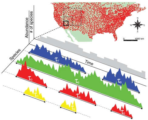
Understanding local extinction processes has gained urgency as the number of threatened species increases throughout the world because of factors such as habitat destruction or climate change (1–5), but a synthesis of theory and empirical evidence accounting for the relevant ecological dynamics is lacking. In this context, we address here the study of persistence times of trophically equivalent co-occurring species in relation to the spatial scale of observation. The persistence time τ of a species within a geographic region is defined as the time incurred between its emergence and its local extinction (see refs. 6 and 7 and Fig. 1). At a local scale, persistence times are largely controlled by ecological processes operating at short time scales (e.g., population dynamics, dispersal, immigration, and contraction/expansion of species geographic ranges) as local extinctions are dynamically balanced by colonizations (8, 9). At a global scale, originations and extinctions are controlled by mechanisms acting on macroevolutionary time scales.

Fig. 1.

Species persistence times. Persistence time τ within a geographic region is defined as the time incurred between a species’ emergence and its local extinction. Recurrent colonizations of a species define different persistence times. The number of species in the ecosystem as a function of time (gray shaded area) crucially depends on species emergences and persistence times. We analyze two long-term datasets about North America breeding birds (22) and herbaceous plants from Kansas prairies (23). (Inset) Observational routes of the Breeding Bird Survey. Aggregating local information comprised in a given geographic area, we reconstruct species presence–absence time series that allow the estimation of persistence-time distributions.

From a theoretical viewpoint, the simplest baseline model for population dynamics is a random walk without drift, according to which the abundance of a species in a geographic region has the same probability of increasing or decreasing by one individual at every time step. According to this scheme, local extinction is equivalent to a random walker’s first passage to zero, and thus the resulting persistence-time distribution has a power-law decay with exponent 3/2 (10).

A more realistic description can be achieved by accounting for basic ecological processes such as birth, death, migration, and speciation in neutral (11–14) mean-field schemes, as follows. Consider a community of N individuals belonging to different species. At every time step a randomly selected individual dies and space or resources are freed up for colonization. With probability ν the site is taken by an individual of a species not currently present in the system; ν is equivalent to a per-birth diversification rate and it accounts for both speciation and immigration from surrounding communities. With the residual probability 1 - ν the individual who died is replaced by one offspring of an individual randomly sampled within the community (15, 16). As such the probability of colonization by a species depends solely on its relative abundance in the community. The asymptotic behavior of the resulting persistence-time distribution [i.e., p_τ(t)] exhibits a power-law scaling limited by an exponential cutoff:

[1]

with exponent α = 2 (7). In formula 1, time is expressed in generation time units (11); i.e., it has been rescaled such that the birth rate is equal to one. Notably, in the mean-field scheme the probability distribution p_τ(t) depends solely on the diversification rate that accounts for speciation and migration processes and imposes a characteristic time scale 1/ν for local extinctions. Although per-birth speciation rates are not expected to vary with the spatial scale of analysis, per-birth immigration rates are argued to decrease as the spatial scale increases. In fact, the possible sources of migration (chiefly dependent on the geometrical properties of the boundary and the nature of dispersal processes) are argued to scale sublinearly with the community size (17), which in turn is typically linearly proportional to geographic area (2, 8). As continental scales are approached, migration processes (almost) vanish and the diversification rate ultimately reflects only the speciation rate.

From an empirical viewpoint, species and genera persistence times deducted from fossil record data have been suggested to follow either power-law [with nontrivial exponents in the range 1.5–2 (18–20)] or exponential distributions (19, 21). It has been argued, however, that data quality, in particular for species, precludes a critical assessment (7). Also, local analyses of species persistence over ecological time scales suggest power-law distributions with nontrivial exponents (6).

In what follows we provide evidence for power-law behavior, either empirically or from a broad spectrum of theoretical derivations. Implications on emerging macroecological patterns are examined, with special attention to possible biogeographical effects.

Empirical Persistence-Time Distributions

We empirically characterize species persistence-time distributions by analyzing two long-term datasets covering very different spatial scales: (i) a 41-y survey of North American breeding birds (22) and (ii) a 38-y inventory of herbaceous plants from Kansas prairies (23).

The North American Breeding Bird Survey consists of a record of annual abundance of more than 700 species over the 1966–present period along more than 5,000 observational routes. The spatial location of the routes analyzed is shown in Fig. 1. We consider only routes with a latitude less than 50° because density of routes with a long surveyed period drastically decreases above the 50th parallel. Noting that in many regions the survey started only in 1968, we discard the first two years of observations in order to have simultaneous records for all the regions in the system. The spatial extent of the observational routes allows us to analyze species persistence times at different spatial scales. We consider 20 different scales of analysis with linearly increasing values of the square root of the sampled area starting from A = 10,000 km² to A = 3.8·10⁶ km². We also analyze the whole system, which corresponds to an area of A = 7.8·10⁶ km². For every scale of analysis A we consider several overlapping square cells of area A inside the system. A three-dimensional presence–absence matrix P is thus built. Each element p_stc of the matrix is equal to 1 if species s is observed during year t in at least one of the observational routes comprised in cell c; otherwise p_stc = 0. For every scale of analysis we discard the cells that (i) do not have a continuous record for the whole period (41 y) or (ii) have more than 5% of their area falling outside the system. For every cell and every species we measure persistence times from presence–absence time series derived from the second dimension of matrix P. Persistence time is defined as the length of a contiguous sequence of ones in the time series. For every scale of analysis we consider all the measured persistence times regardless of the species they belong to and the cell where they are measured. The effect of possible imperfect detection of species (24) on measured persistence times has also been investigated (see SI Text).

The herbaceous plant dataset (23) comprises a series of 51 quadrats of 1 m² from mixed Kansas grass prairies where all individual plants were mapped every year from 1932 to 1972. In order to meet the data quality standard required for our analysis as discussed above for the breeding bird data, we discard 10 quadrats and the first three years of observations. Because of the limited number of observational plots in the herbaceous plant dataset, we limit our analysis to quadrat spatial scale A = 1 m². Analogously to the previous case, we reconstruct the matrix P from presence–absence data for every species, year, and quadrat.

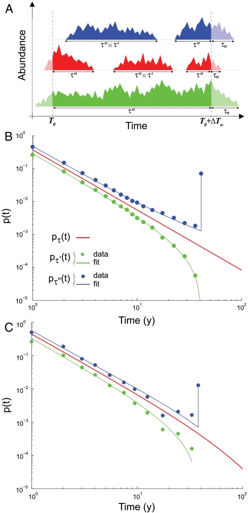
Note that, when dealing with empirical survey data, the effect of the finiteness of the observational time window on the measured species persistence times must be properly taken into account. To this end, we have developed tools to extend the inference of persistence-time distributions for periods longer than the observational window. In particular, we analytically derive, given the persistence-time probability density function, the distribution of two additional variables that can actually be measured from empirical data: (i) the persistence times τ^′ of species that emerge and go locally extinct within the observed time window ΔT_w and (ii) the variable τ^′′ that comprises τ^′ and all the portions of species persistence times that are partially seen inside the observational time window but start or/and end outside (Fig. 2A and Materials and Methods). The finiteness of the time window imposes a cutoff to p_τ^′(t). On the contrary p_τ^′′(t) has an atom of probability in t = ΔT_w corresponding to the fraction of species that are always present during the observational time. By matching analytical and observational distributions for p_τ^′(t) and p_τ^′′(t), it is possible to infer the persistence-time distribution p_τ(t). The scaling exponent and the diversification rate for the herbaceous plant persistence-time distributions have been determined with a simultaneous nonlinear fit of observational and analytical p_τ^′(t) and p_τ^′′(t). Confidence intervals are equal to the standard error of the fit. For breeding birds, we repeat the nonlinear fit for different spatial scales of analysis. The reported scaling exponent and the confidence interval have been obtained by averaging results across spatial scales.

Fig. 2.

Empirical persistence-time distributions. (A) A schematic representation of the variables that can be measured from empirical data over a time window ΔT_w: τ^′, persistence times that start and end inside the observational window, and τ^′′ , which comprises τ^′ and all the portions of persistence times seen inside the time window that start or/and end outside. Times to local extinction τ_e are also presented. (B) Breeding birds and (C) herbaceous plants probability density function p(t) of τ^′ (green), τ^′′ (blue), and persistence time τ (red). Filled circles and solid lines show observational distributions and fits, respectively. The best fit is achieved with p_τ(t) ∝ t^-α with α = 1.83 ± 0.02 and α = 1.78 ± 0.08 for breeding birds and herbaceous plants, respectively. Note that previous estimates (6) for B are revisited here in the light of the tools developed and of a longer dataset. The spatial scale of analysis is A = 10,000 km² and ΔT_w = 41 y for B and A = 1 m² and ΔT_w = 38 y for C. The finiteness of the time window imposes a cutoff to p_τ^′(t) and an atom of probability in t = ΔT_w to p_τ^′′(t), which corresponds to the fraction of species that are always present during the observational time. p_τ(t) and p_τ^′(t) have been shifted in the log–log plot for clarity.

Remarkably, the persistence times of breeding birds at different spatial scales of analysis and of herbaceous plants prove to be best fitted by a power-law distribution with an exponent α = 1.83 ± 0.02 and α = 1.78 ± 0.08, respectively (Fig. 2 B and C). It is important to note that both scaling coefficients derived empirically are significantly different from the predictions of the existing baseline models discussed above (the random-walk persistence time yields an exact exponent α = 3/2; the mean-field model yields α = 2).

Theoretical Persistence-Time Distributions

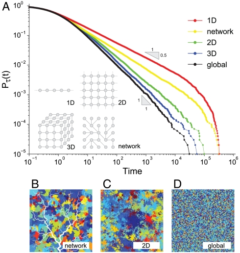
In this section we provide a theoretical rationale for the universality of the scaling behavior of persistence-time distributions with respect to the topology of the interactions allowed by the environmental matrix. In particular, we provide evidence on how nontrivial exponents of the type observed empirically can be reproduced by simple theoretical models once dispersal limitation and the actual network of spatial connections are taken into account. We have implemented the neutral game described above in regular one-, two-, and three-dimensional lattices in which every site represents an individual (15, 16). We have also explored the patterns emerging from the application of the model to dendritic structures mimicking riverine ecosystems where dispersal processes and ecological organization are constrained by the network structure. Indeed, many features of riverine ecosystems have been shown to be affected by the connectivity of river networks (25, 26). In particular, river geometry has been studied in relation to extinction risk (27), migration processes (28), persistence of amphibian populations (29), macroinvertebrate dispersal (30), and freshwater fish biodiversity (14, 31). For general calculations of the topological structure and metric properties relevant to dendritic ecological corridors, we employ the features of optimal channel networks (OCNs) (32). They hold fractal characteristics known to closely conform to the scaling of real networks (33). Among the advantages of the use of OCNs, one recalls the possibility to fit one such construct into any assigned domain (e.g., a square, Fig. 3), thus allowing exactly the same size and number of nodes of a two-dimensional lattice to be endowed with altered directionality of connections. To account for limited dispersal effects, we allow only the offsprings of the nearest neighbors of the individual who died to possibly colonize the empty site. In the networked landscape the neighborhood of a site is defined by the closest upstream and downstream sites. Limited dispersal promotes the clumping in space of species, which enhances their coexistence and survival probability (16, 34). Indeed we find that in all the considered landscapes, persistence-time distributions still follow a power-law behavior characterized by smaller, nontrivial scaling exponents (namely α = 1.92 for the 3D, α = 1.82 for the 2D, α = 1.62 for the OCN, and α = 1.50 for the 1D landscape, Fig. 3) limited by an exponential cutoff. Remarkably, the exponent obtained via simulation in a two-dimensional landscape (α = 1.82 ± 0.01) is close to those found in both breeding birds and herbaceous plants datasets (α = 1.83 ± 0.02 and α = 1.78 ± 0.08, respectively).

Fig. 3.

Persistence-time distributions are dependent on the structure of the spatial interaction networks. (A) Persistence-time exceedance probabilities P_τ(t) (probability that species’ persistence times τ be ≥t) for the neutral individual-based model (15, 16) with nearest-neighbor dispersal implemented on the different topologies shown in the inset. Note that in the power-law regime if p_τ(t) scales as t^-α, P_τ(t) ∝ t^-α+1. The scaling exponent α is equal to 1.50 ± 0.01 for the one-dimensional lattice (red), α = 1.62 ± 0.01 for the networked landscape (yellow), 1.82 ± 0.01 and 1.92 ± 0.01, respectively, for the 2D (green) and 3D (blue) lattices. Errors are estimated through the standard bootstrap method. The persistence-time distribution for the mean-field model (global dispersal) reproduces the exact value α = 2 (black curve). For all simulations ν = 10^-5 and time is expressed in generation time units (11). (Bottom) Sketches of the color-coded spatial arrangements of species in a networked landscape (B), in a two-dimensional lattice with nearest-neighbor dispersal (C), and with global dispersal (D).

We also study how persistence-time distributions deducted from the theoretical model change with dispersal broader than nearest neighbors (see SI Text). As expected, as long as the mean dispersal distance remains small with respect to the system size, the distribution eventually ends up scaling as the one predicted by the nearest-neighbors dispersal. We also relax the neutral assumption by implementing an individual-based competition/survival trade-off model (16). Specifically, species with higher mortality rates are assumed to hold less competitive ability to colonize empty sites (2, 35). It is important to note that the trade-off model also exhibits power-law persistence-time distribution with exponents indeed close to those shown by the neutral model (see SI Text). Our theoretical results are thus robust with respect both to changes in the dispersal range and to relaxations of the neutrality assumptions. This confirms our expectation that a power-law distribution for species persistence times is the result of emergent behaviors independent of fine ecological details, thus supporting the neutral assumption that effective interaction strength among species is weak (36) and does not significantly constrain the dynamics of ecosystems. We also note that our results are not seen as a test for the neutrality hypothesis for breeding birds or herbaceous plants dynamics, but rather as tools to reveal emerging universal and macroscopic patterns (37, 38).

Discussion and Conclusions

In the previous section we established a hierarchy of scaling exponents ranging from the smallest, proper to 1D interactions, to larger values namely for directional (network-like), 2D, and 3D dispersals. We thus suggest that the coherence of the empirical scalings would stem from the two-dimensional isotropic nature of the environmental matrix available to the ecological processes relevant to both breeding birds and herbaceous plants.

We also suggest that species persistence-time distribution, owing to its robustness and scale-invariant character, is a synthetic descriptor of ecosystem dynamics and of biodiversity. In fact, other key macroecological patterns are intimately related to the persistence-time distribution. A first clear example is the direct link with ecosystem diversity, as explained below. In our framework species emerge as a point Poisson process with rate λ = νN and last for a persistence time τ. The mean number of species S in the system at a given time is therefore S = λ〈τ〉 (39) where 〈τ〉 is the mean persistence time. Therefore, the smaller exponents found, say, for networked environments with respect to two-dimensional ones, imply longer mean persistence and, in turn, higher diversity. This echoes recent results suggesting a higher diversity of freshwater versus marine ray-finned fishes (40, 41).

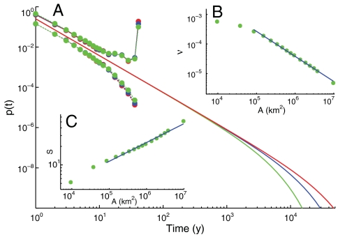
Another evidence of the effective way in which species persistence-time distribution can characterize ecosystem diversity is the link with the species-area relationship, which characterizes the increase in the observed number of species with increasing sample area. The spatial extent of the breeding bird dataset and the tools developed for the data analysis allow us to study how the persistence-time distribution depends on the spatial scale of analysis (Fig. 4A). As expected, while the scaling exponent remains the same, the diversification rate ν decreases with the geographic area A and is found to closely follow a scaling relation of the type ν ∝ A^-β, with β = 0.84 ± 0.01 (Fig. 4B), for a wide range of areas. This scaling form of the cutoff time scale 1/ν can be related to the species-area relationship. Assuming that the number of individuals scales isometrically with the sampled geographic area (2, 8), i.e., N ∝ A, and given that 〈τ〉 = ∫tp_τ(t)dt ∝ ν^α-2 (see SI Text) one gets

[2]

The observational values β = 0.84 ± 0.01 and α = 1.83 ± 0.02 give an exponent z = 0.30 ± 0.02, which is close to the species-area relation measured directly on the data for the same range of areas (z = 0.31 ± 0.02, Fig. 4C). Conversely, one could have used the observed species-area exponent to infer the scaling properties of the diversification rate.

Fig. 4.

Biogeography of species persistence time. (A) Observational distributions p_τ^′(t) and p_τ^′′(t) (interpolated solid circles) for the breeding bird dataset and corresponding fitted persistence-time distributions p_τ(t) ∝ t^-αe^-νt (solid lines) for different scales of analysis: Area A = 8.5·10⁴ km² (green), A = 3.4·10⁵ km² (blue), A = 9.5·10⁵ km² (red). ν(A) provides the cutoff for the distribution, whose scaling exponent is unaffected by geographic area. Note that the position of the cutoff of p_τ(t) is inferred from the estimate of the atom of probability of p_τ^′′(t), which is more sensitive to the scale of analysis. (B) Scaling of the diversification rate ν with the geographic area ν ∝ A^-β, β = 0.84 ± 0.01. (C) Empirical species-area relationship (SAR). The plot shows the mean number of species S found in moving squares of size A. We find S ∝ A^z, z = 0.31 ± 0.02. Slope and confidence interval have been obtained averaging 41 SARs, one per year of observation.

Finally, from a conservation perspective, a meaningful assessment of species’ local extinction rates is deemed valuable. We propose the distribution of the times to local extinction τ_e (Fig. 2A) as a tool to quantify the dynamical evolution of the species assembly currently observed within a given geographic area. Mathematically, τ_e is defined as the time to local extinction of a species randomly sampled from the system, regardless of its current abundance. When formula 1 holds for persistence times, the distribution of the times to local extinction p_τe(t) is shown to scale as p_τe(t) ∝ t^1-αe^-νt (see Materials and Methods). Therefore, not only do the developed theoretical and operational tools allow to infer the scaling behavior of persistence times, but also of the time to local extinction even from relatively short observational windows. Although these patterns cannot provide information about the behavior of a specific species or of a particular patch inside the ecosystem considered (e.g., a biodiversity hot spot), they can effectively describe the overall dynamical evolution of the ecosystem diversity. In particular, the scaling behavior allows us to extrapolate species persistence-time distributions for wide geographic areas, which are hard to estimate, from measures of persistence on smaller areas, which are, on the contrary, more practical and feasible. We thus conclude that the biogeographical characters of species persistence, stemming from the structure of the spatial interaction networks and from local constraints to species emergence rates, add a previously undescribed ingredient to a rich literature bearing major implications for the inventory of life on Earth.

Materials and Methods

Inference of the Persistence-Time Distribution from a Finite Observational Period.

The exact derivation of the probability distribution of the variables τ^′ and τ^′′ (Fig. 2A) follows. In this theoretical framework, the probability νdt of observing a diversification event in a time step dt is assumed to be a constant; thus species emergence in the system due to migration or speciation is seen as a uniform point Poisson process with rate λ = νN (where N is total number of individuals in the system and λ has the dimension of the inverse of a generation time). We term t₀ the emergence time of a species in the system, and T₀ and T_f = T₀ + ΔT_w the beginning and the end of the observational time window, respectively. A species emerged at time t₀ will be continuously present in a geographic region for its persistence time τ until its local extinction at time t₀ + τ.

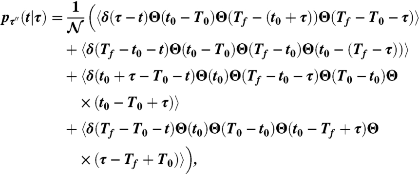
We first analyze the distribution of τ^′′, the most complex case. The variable τ^′′ can be expressed as a function of the random variables τ and t₀, which are probabilistically characterized. We can distinguish four different cases (Fig. 2A):

1. the species emerges and goes locally extinct within the time window;

2. the species emerges during the observations and it is still present at the end of the time window;

3. the species emerges before the beginning of the observations and goes locally extinct within the time window;

4. the species is always present for all the duration of the observations;

or, mathematically,

We express the probability of observing τ^′′ conditional on a persistence time of duration τ as

[3]

where the operator 〈·〉 is the ensemble average with respect to the random variable t₀, δ(x) and Θ(x) are the Dirac delta distribution and the Heaviside function, respectively. is the normalization constant.

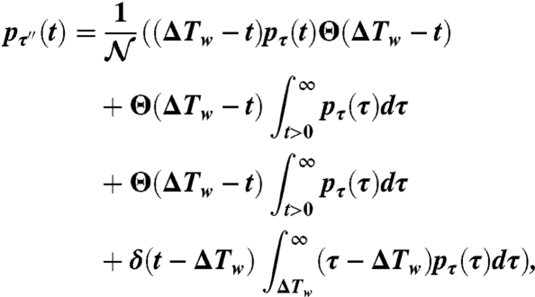
When comparing analytical and observational distributions, we assume that the system is at stationarity and unaffected by initial conditions; i.e., T₀ is far from the beginning of the process. Mathematically this is obtained taking the limit T₀,T_f → +∞ with T_f - T₀ = ΔT_w. By solving the ensemble averages and by marginalizing with respect to τ, Eq. 3 finally takes the form (see SI Text for a step-by-step derivation)

[4]

where simplifies to

with being the exceedance cumulative distribution of the persistence-time probability density function.

The variable τ^′ comprises only the first of the four cases listed in Eq. 3. Thus the probability distribution p_τ^′(t) follows directly from the first term of Eq. 4,

where the normalization constant is equal to

which completes the derivation.

Distribution of Times to Local Extinction.

We term τ_e the time to local extinction of a species randomly sampled among the observed assembly at a certain time T (Fig. 2A). Analogously to the derivation described above, we can express τ_e as

We then express the probability distribution of the times to local extinction conditioned to a persistence time τ as

where the constant ensures proper normalization. Solving the ensemble average operators yields

Marginalizing over τ and considering the system at stationarity (T → +∞), we finally obtain

[5]

where is simply 〈τ〉. Eq. 5 allows us to derive the distribution of the times to local extinction given the persistence-time distribution. Particularizing now to the case of persistence-time distributions of the shape p_τ(t) ∝ t^-αe^-νt, Eq. 5 translates into p_τe(t) ∝ t^1-αe^-νt.

References

- 1.Diamond J. The present, past and future of human-caused exctinctions. Philos Trans R Soc London B. 1989;325:469–477. doi: 10.1098/rstb.1989.0100. [DOI] [PubMed] [Google Scholar]
- 2.Brown JH. Macroecology. Chicago: Univ Chicago Press; 1995. [Google Scholar]
- 3.Thomas C, et al. Extinction risk from climate change. Nature. 2004;427:145–148. doi: 10.1038/nature02121. [DOI] [PubMed] [Google Scholar]
- 4.Svenning J.-C, Condit R. Biodiversity in a warmer world. Science. 2008;322:206–207. doi: 10.1126/science.1164542. [DOI] [PubMed] [Google Scholar]
- 5.May RM. Ecological science and tomorrow’s world. Philos Trans R Soc London B. 2010;365:41–47. doi: 10.1098/rstb.2009.0164. [DOI] [PMC free article] [PubMed] [Google Scholar]
- 6.Keitt T, Stanley H. Dynamics of North American breeding bird populations. Nature. 1998;393:257–260. [Google Scholar]
- 7.Pigolotti S, Flammini A, Marsili M, Maritan A. Species lifetime distribution for simple models of ecologies. Proc Natl Acad Sci USA. 2005;102:15747–15751. doi: 10.1073/pnas.0502648102. [DOI] [PMC free article] [PubMed] [Google Scholar]
- 8.MacArthur RH, Wilson EO. The Theory of Island Biogeography. Princeton, NJ: Princeton Univ Press; 1967. [Google Scholar]
- 9.Ricklefs R. Community diversity—Relative roles of local and regional processes. Science. 1987;235:167–171. doi: 10.1126/science.235.4785.167. [DOI] [PubMed] [Google Scholar]
- 10.Chandrasekhar S. Stochastic problems in physics and astronomy. Rev Mod Phys. 1943;15:1–89. [Google Scholar]
- 11.Hubbell S. The Unified Theory of Biodiversity and Biogeography. Princeton, NJ: Princeton Univ Press; 2001. [Google Scholar]
- 12.Volkov I, Banavar J, Hubbell S, Maritan A. Neutral theory and relative species abundance in ecology. Nature. 2003;424:1035–1037. doi: 10.1038/nature01883. [DOI] [PubMed] [Google Scholar]
- 13.Alonso D, Etienne RS, McKane AJ. The merits of neutral theory. Trends Ecol Evol. 2006;21:451–457. doi: 10.1016/j.tree.2006.03.019. [DOI] [PubMed] [Google Scholar]
- 14.Muneepeerakul R, et al. Neutral metacommunity models predict fish diversity patterns in Mississippi–Missouri basin. Nature. 2008;453:220–222. doi: 10.1038/nature06813. [DOI] [PubMed] [Google Scholar]
- 15.Durrett R, Levin S. Spatial models for species-area curves. J Theor Biol. 1996;179:119–127. [Google Scholar]
- 16.Chave J, Muller-Landau H, Levin S. Comparing classical community models: Theoretical consequences for patterns of diversity. Am Nat. 2002;159:1–23. doi: 10.1086/324112. [DOI] [PubMed] [Google Scholar]
- 17.Chisholm RA, Lichstein JW. Linking dispersal, immigration and scale in the neutral theory of biodiversity. Ecol Lett. 2009;12:1385–1393. doi: 10.1111/j.1461-0248.2009.01389.x. [DOI] [PubMed] [Google Scholar]
- 18.Sneppen K, Bak P, Flyvbjerg H, Jensen M. Evolution as a self-organized critical phenomenon. Proc Natl Acad Sci USA. 1995;92:5209–5213. doi: 10.1073/pnas.92.11.5209. [DOI] [PMC free article] [PubMed] [Google Scholar]
- 19.Solé R, Bascompte J. Are critical phenomena relevant to large-scale evolution? Proc R Soc London Ser B. 1996;263:161–168. doi: 10.1098/rspb.1996.0026. [DOI] [PubMed] [Google Scholar]
- 20.Newman M, Sibani P. Extinction, diversity and survivorship of taxa in the fossil record. Proc R Soc London Ser B. 1999;266:1593–1599. [Google Scholar]
- 21.VanValen L. A new evolutionary law. Evol Theor. 1973;1:1–30. [Google Scholar]
- 22.Department of the Interior Geological Survey, Patuxent Wildlife Research Center, Laurel, MD. North American Breeding Bird Survey. http://www.pwrc.usgs.gov/bbs.
- 23.Adler PB, Tyburczy WR, Lauenroth WK. Long-term mapped quadrats from Kansas prairie: Demographic information for herbaceous plants. Ecology. 2007;88:2673–2673. [Google Scholar]
- 24.Alpizar-Jara R, et al. The relationship between species detection probability and local extinction probability. Oecologia. 2004;141:652–660. doi: 10.1007/s00442-004-1641-0. [DOI] [PubMed] [Google Scholar]
- 25.Grant EHC, Lowe WH, Fagan WF. Living in the branches: Population dynamics and ecological processes in dendritic networks. Ecol Lett. 2007;10:165–175. doi: 10.1111/j.1461-0248.2006.01007.x. [DOI] [PubMed] [Google Scholar]
- 26.Rodriguez-Iturbe I, Muneepeerakul R, Bertuzzo E, Levin SA, Rinaldo A. River networks as ecological corridors: A complex systems perspective for integrating hydrologic, geomorphologic, and ecologic dynamics. Water Resour Res. 2009;45:W01413. [Google Scholar]
- 27.Fagan W. Connectivity, fragmentation, and extinction risk in dendritic metapopulations. Ecology. 2002;83:3243–3249. [Google Scholar]
- 28.Campos D, Fort J, Mendez V. Transport on fractal river networks: Application to migration fronts. Theor Popul Biol. 2006;69:88–93. doi: 10.1016/j.tpb.2005.09.001. [DOI] [PubMed] [Google Scholar]
- 29.Grant EHC, Nichols JD, Lowe WH, Fagan WF. Use of multiple dispersal pathways facilitates amphibian persistence in stream networks. Proc Natl Acad Sci USA. 2010;107:6936–6940. doi: 10.1073/pnas.1000266107. [DOI] [PMC free article] [PubMed] [Google Scholar]
- 30.Brown BL, Swan CM. Dendritic network structure constrains metacommunity properties in riverine ecosystems. J Anim Ecol. 2010;79:571–580. doi: 10.1111/j.1365-2656.2010.01668.x. [DOI] [PubMed] [Google Scholar]
- 31.Bertuzzo E, et al. On the geographic range of freshwater fish in river basins. Water Resour Res. 2009;45 [Google Scholar]
- 32.Rodriguez-Iturbe I, et al. Fractal structures as least energy patterns—The case of river networks. Geophys Res Lett. 1992;19:889–892. [Google Scholar]
- 33.Rinaldo A, et al. Minimum energy and fractal structures of drainage networks. Water Resour Res. 1992;28:2183–2195. [Google Scholar]
- 34.Kerr B, Riley M, Feldman M, Bohannan B. Local dispersal promotes biodiversity in a real-life game of rock-paper-scissors. Nature. 2002;418:171–174. doi: 10.1038/nature00823. [DOI] [PubMed] [Google Scholar]
- 35.Tilman D. Competition and biodiversity in spatially structured habitats. Ecology. 1994;75:2–16. [Google Scholar]
- 36.Volkov I, Banavar JR, Hubbell SP, Maritan A. Inferring species interactions in tropical forests. Proc Natl Acad Sci USA. 2009;106:13854–13859. doi: 10.1073/pnas.0903244106. [DOI] [PMC free article] [PubMed] [Google Scholar]
- 37.Solé R, Alonso D, McKane A. Self-organized instability in complex ecosystems. Philos Trans R Soc London B. 2002;357:667–681. doi: 10.1098/rstb.2001.0992. [DOI] [PMC free article] [PubMed] [Google Scholar]
- 38.Pueyo S, He F, Zillio T. The maximum entropy formalism and the idiosyncratic theory of biodiversity. Ecol Lett. 2007;10:1017–1028. doi: 10.1111/j.1461-0248.2007.01096.x. [DOI] [PMC free article] [PubMed] [Google Scholar]
- 39.Rodriguez-Iturbe I, Cox D, Isham V. Some models for rainfall based on stochastic point-processes. Proc R Soc London Ser A. 1987;410:269–288. [Google Scholar]
- 40.de Aguiar MAM, Baranger M, Baptestini EM, Kaufman L, Bar-Yam Y. Global patterns of speciation and diversity. Nature. 2009;460:384–U98. doi: 10.1038/nature08168. [DOI] [PubMed] [Google Scholar]
- 41.Moyle P, Chech J. An Introduction to Ichthyology. 5th Ed. San Francisco: Benjamin Cummings; 2003. [Google Scholar]
Associated Data
This section collects any data citations, data availability statements, or supplementary materials included in this article.