Abstract
Purpose: In comparison with conventional filtered backprojection (FBP) algorithms for x-ray computed tomography (CT) image reconstruction, statistical algorithms directly incorporate the random nature of the data and do not assume CT data are linear, noiseless functions of the attenuation line integral. Thus, it has been hypothesized that statistical image reconstruction may support a more favorable tradeoff than FBP between image noise and spatial resolution in dose-limited applications. The purpose of this study is to evaluate the noise-resolution tradeoff for the alternating minimization (AM) algorithm regularized using a nonquadratic penalty function.
Methods: Idealized monoenergetic CT projection data with Poisson noise were simulated for two phantoms with inserts of varying contrast (7%–238%) and distance from the field-of-view (FOV) center (2–6.5 cm). Images were reconstructed for the simulated projection data by the FBP algorithm and two penalty function parameter values of the penalized AM algorithm. Each algorithm was run with a range of smoothing strengths to allow quantification of the noise-resolution tradeoff curve. Image noise is quantified as the standard deviation in the water background around each contrast insert. Modulation transfer functions (MTFs) were calculated from six-parameter model fits to oversampled edge-spread functions defined by the circular contrast-insert edges as a metric of local resolution. The integral of the MTF up to 0.5 lp∕mm was adopted as a single-parameter measure of local spatial resolution.
Results: The penalized AM algorithm noise-resolution tradeoff curve was always more favorable than that of the FBP algorithm. While resolution and noise are found to vary as a function of distance from the FOV center differently for the two algorithms, the ratio of noises when matching the resolution metric is relatively uniform over the image. The ratio of AM-to-FBP image variances, a predictor of dose-reduction potential, was strongly dependent on the shape of the AM’s nonquadratic penalty function and was also strongly influenced by the contrast of the insert for which resolution is quantified. Dose-reduction potential, reported here as the fraction (%) of FBP dose necessary for AM to reconstruct an image with comparable noise and resolution, for one penalty parameter value of the AM algorithm was found to vary from 70% to 50% for low-contrast and high-contrast structures, respectively, and from 70% to 10% for the second AM penalty parameter value. However, the second penalty, AM-700, was found to suffer from poor low-contrast resolution when matching the high-contrast resolution metric with FBP.
Conclusions: The results of this simulation study imply that penalized AM has the potential to reconstruct images with similar noise and resolution using a fraction (10%–70%) of the FBP dose. However, this dose-reduction potential depends strongly on the AM penalty parameter and the contrast magnitude of the structures of interest. In addition, the authors’ results imply that the advantage of AM can be maximized by optimizing the nonquadratic penalty function to the specific imaging task of interest. Future work will extend the methods used here to quantify noise and resolution in images reconstructed from real CT data.
Keywords: computed tomography, alternating minimization, nonquadratic regularization, noise, resolution
INTRODUCTION
Conventional filtered backprojection (FBP) algorithms1 provide an exact solution to the inverse problem of computed tomography (CT) under the assumption that a complete set of noiseless transmission measurements are available, which are linear functions of the attenuation line integral through the patient. However, phenomena such as measurement noise,2 scatter,3, 4 beam-hardening,5 and high-contrast edge effects6 lead to data nonlinearity and artifacts such as streaking and cupping in the reconstructed image. The classic expectation-maximization algorithm of Lange and Carson7 was formed around the statistical nature of x-ray CT data and provided the foundation for a class of statistically motivated algorithms that can directly incorporate many of these nonlinear signal-formation processes into their data models. The reader is referred to Fessler’s8 overview of statistical image reconstruction (SIR) algorithm methodology. The promise of better image quality via a more realistic modeling of the underlying CT physics has motivated many investigations of statistical algorithms, despite the extensive computational resources they demand.
It seems intuitive that SIR algorithms that explicitly model CT-signal statistics would be able to reconstruct images with less noise than FBP from the same noisy projection data set. However, it is known that the image most likely to match the measured data suffers from excessive image noise.9, 10 A widely used approach to suppress image noise in statistically based reconstruction algorithms is to modify the objective function to incorporate some a priori assumptions about the scan subject, e.g., the local neighborhood penalty function investigated by this study that enforces the assumption of image smoothness. As with any noise-reduction method, there is an associated cost. In CT image reconstruction, one of the most tangible costs of noise reduction is loss of spatial resolution. The degradation of spatial resolution associated with noise reduction constitutes what we will refer to as the noise-resolution tradeoff.
An algorithm with a better noise-resolution tradeoff would have an advantage in a number of clinical situations. Better noise-resolution tradeoff means that an algorithm can reconstruct images from the same data with either less image noise for similar resolution or better image resolution for similar image noise. By extension, an algorithm that provides a noise-resolution tradeoff advantage could provide images of comparable image quality, in terms of both noise and resolution, from data with more noise, i.e., data acquired with lower imaging dose, an important area of concern in diagnostic radiology.11 Pediatric imaging and lung cancer screening are relevant clinical scenarios where improved reconstruction techniques for low dose CT would be clinically valuable.
SIR algorithms could also find use in quantitative CT applications. The very specific application of estimating the photon cross-sections from dual-energy measurements has been shown to be extremely sensitive to the accuracy of the measured CT values.12 Cupping and streaking artifacts from data nonlinearities such as beam-hardening and scatter represent systematic shifts in CT image intensity. The focus of this work is to assess the suppression of random errors, i.e., image noise. Measurement noise can be reduced by averaging over a large number of pixels within a homogeneous region but at the expense of reduced spatial resolution. This may, in turn, introduce large systematic dose-calculation errors in low energy photon-emitting treatment modalities that exhibit large dose gradients, such as brachytherapy. An algorithm that can provide superior noise-resolution tradeoff may prove useful in such quantitative CT applications where both low noise and high resolution are important.
In this work, we assess the noise-resolution tradeoff, in comparison with FBP, for the alternating minimization (AM) algorithm,13 which provides for an exact update solution to the objective function. A nonquadratic penalty function is used to regularize the AM algorithm and to tradeoff noise and resolution. Previous investigators have assessed the noise-resolution tradeoff to evaluate SIR algorithms using parabolic surrogates to model the Poisson log-likelihood,14, 15 adaptive statistical sinogram smoothing techniques,14 and iterative reconstruction algorithms for cone-beam CT imaging geometries.16, 17 In contrast with these previous studies that have quantified resolution only for high-contrast structures, our study investigates the impact of structure contrast on the reported noise-resolution tradeoff. An ideal monoenergetic simulation environment is used to avoid artifacts arising from data nonlinearity, such as scattered radiation and beam-hardening, the goal being to isolate the smoothing effects of the two algorithms. In this way, we form a baseline of noise-resolution tradeoff performance for the FBP and alternating minimization algorithms for ideal Poisson-counting projection data. Future work will extend the methods for the quantification of noise and resolution in this paper to images reconstructed from real CT data.
MATERIALS AND METHODS
CT image reconstruction
Penalized AM reconstruction
The penalized monoenergetic version of the alternating minimization algorithm is used to reconstruct the synthetic projection data. The AM algorithm reformulates the classic maximization of the Poisson log-likelihood as an alternating minimization of Csiszar’s18I-divergence between the measured data d and the expected data means g
| (1) |
where μ′ is the current image estimate. The I-divergence is the negative of the log-likelihood, meaning that minimization of the I-divergence is identical to the maximization of the log-likelihood. For full details of the alternating minimization algorithm, the reader is referred to O’Sullivan’s 2007 paper.13 A log-cosh penalty term is included in the AM algorithm’s objective function to enforce our a priori assumption of image smoothness
| (2) |
where α controls the relative weight of the penalty function. The roughness penalty computes a penalty for a pixel x as a function of the pixel intensities in the local neighborhood N(x). The penalty chosen for this study is defined as
| (3) |
The neighboring pixels are weighted as 1.0 for directly adjacent pixels and 0 for all other pixels
| (4) |
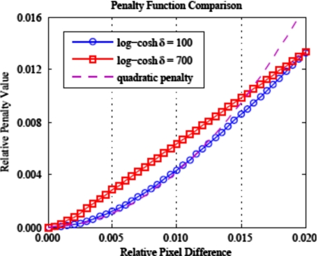
Purely quadratic penalty functions effectively suppress noise, but tend to blur high-contrast edges as the penalty grows quickly for large pixel intensity differences. The continuously defined edge-preserving log-cosh function19 is similar to a Huber penalty,20 which is quadratic for small pixel-to-pixel variations, so as to suppress noise, and linear for larger variations, so as to preserve edge boundaries. The parameter δ controls the pixel intensity difference for which the penalty transitions from quadratic to linear growth. Increasing δ causes the transition to linear growth to occur at smaller intensity differences. Two different values of δ are investigated to study the effect on image noise and resolution. We let AM-100 denote images reconstructed with the penalized AM algorithm with δ=100, which transitions to linear penalty growth for pixel differences approximately 50% of the water background. AM-700 denotes the AM algorithm using a log-cosh penalty with δ=700, which has a growth transition for pixel differences around 10% of background. Figure 1 plots both of the log-cosh penalties investigated in this work and a quadratic penalty function for comparison. Note that the Lagrange multipliers used in Fig. 1 were chosen purely for plotting purposes to showcase the different penalty growth. Values of α for AM-700 nearly an order of magnitude smaller than for AM-100 were necessary to reconstruct images with acceptable quality. AM-100 and AM-700 represent two bounds of potential clinically relevant penalty parameter value choices: AM-100 is closer in shape to a quadratic penalty and AM-700 is closer in shape to a linear penalty. Results for δ values between 100 and 700 would reasonably be expected to lie between the two presented parameter values.
Figure 1.
Comparison of penalty function shape for the two log-cosh penalties investigated in this work and a quadratic penalty. Quadratic penalty functions grow too quickly for large pixel differences and consequently overblur high-contrast edges. Note that the log-cosh penalties are scaled (α) for plotting purposes and do not correspond to the values used in simulation.
To evaluate the tradeoff between image noise and resolution, a set of images was reconstructed with varying log-cosh penalty Lagrange multipliers [α in Eq. 2]. Here we use the term smoothing strength to refer to both the Lagrange multiplier α for the AM algorithm and the full-width at half maximum (FWHM) of the Gaussian-modified ramp filter in the FBP algorithm described in Sec. 2A2. For each data case, an unpenalized AM image is reconstructed as a performance baseline. Both penalty function parameter values of the alternating minimization algorithm were run for 250 iterations with 22 ordered subsets, used to increase the convergence rate.21 The number of iterations was chosen from preliminary simulations that showed the images were well converged.
Filtered backprojection reconstruction
Weighted filtered backprojection as described in Kak and Slaney1 is used to backproject the filtered fan beam projection data. The filter H(f) is a modified ramp filter defined in frequency space as
| (5) |
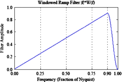
Here s is a constant scale factor that ensures the image intensities represent the correct units of linear attenuation (mm−1) and |f| is the ramp function. The window function that causes the ramp filter to roll off at f≥0.9⋅fN (fN=Nyquist frequency) with a raised cosine function to suppress high-frequency noise is given by
| (6) |
Figure 2 displays the windowed ramp filter. The cosine roll-off in the window function was incorporated to suppress high-frequency ringing artifacts observed in prior simulations at Washington University when a rectangular window function was employed. The frequency at which the cosine roll-off kicks in (90% of Nyquist) was chosen as the highest frequency that suppressed the ringing artifacts in order to retain as much high-frequency content as possible. When compared side-by-side to reconstructions from the proprietary Siemens FBP, trained observers were unable to distinguish which FBP implementation was used for each image. G(f) is the Fourier transform of a Gaussian smoothing kernel that further reduces the amplitude of high spatial frequencies. A series of images with varying levels of noise and resolution is achieved by varying the FWHM of the Gaussian smoothing kernel. For consistency, the system matrix used for the filtered backprojection algorithm is the same as that used for the penalized AM algorithm.
Figure 2.
Windowed ramp filter (no Gaussian smoothing kernel included). Ramp filter is rolled off for frequencies≥90% of fN with a cosine function to suppress high-frequency noise. This filter was chosen in preliminary simulations to reconstruct images that are qualitatively indistinguishable from Siemens clinical images.
Simulated projection data
Virtual CT system
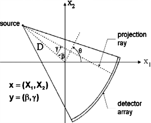
The virtual third generation CT system (Fig. 3) is composed of 1056 gantry positions (β) equally spaced around a full 360° rotation. There are 384 detectors (γ), each subtending an arc angle of 4.0625 min. The source-to-isocenter distance is 570 mm and the source-to-detector distance is 1005 mm. This gives a virtual detector width of 1.2 mm and a projected width at isocenter of 0.67 mm. The image space x is composed of 512×512 square pixels with a length of 0.5 mm on a side, providing a field-of-view (FOV) of 256 mm.
Figure 3.
Third generation virtual CT geometry. Square pixels, 0.5 mm on a side, compose the image space denoted by x. The rays connecting source angle β and detector index γ form the sinogram space y.
We simulate monoenergetic projection data with no scattering to avoid beam-hardening and scatter artifacts in the image reconstruction. Simulated projection data are generated by integrating the ray-traces through the analytically defined phantoms over the detector area
| (7) |
The phantom image μi is defined as a superposition of i analytically defined ellipses. I0 is the number of incident photons on the scan subject and li(γ′) is the analytical path length through the ith ellipse of uniform composition along the ray γ′. A data-model mismatch is present as the data are generated using an analytical forward projector and the reconstruction algorithms use discrete projection. The artifacts from this mismatch are minimal and methods to avoid contamination in the image noise and resolution metrics are discussed in Sec. 2C.
Simple Poisson noise is included in the analytically ray-traced, noiseless sinogram data by randomly varying the incident photon fluence I0. Though CT-signal statistics have been shown to follow the compound Poisson distribution,22 previous literature has shown that approximating this more complex distribution by the simple Poisson distribution, assumed by AM, does not significantly affect image quality.23 An incident fluence of 100 000 photons per detector leads to a percent standard deviation of ∼0.3% for unattenuated source-detector rays, which approximates experimentally observed noise levels in projection data exported from our Philips Brilliance Big Bore CT simulator using a typical clinical scanning protocol (120 kVp, 325 mA s, and 0.75 mm slice thickness). To investigate the impact of projection noise on the noise-resolution tradeoff, noisy sinograms are generated for I0=25 000 photons per detector (25k projection noise case) and I0=200 000 photons per detector (200k projection noise case), which represent low dose and low noise imaging protocols, respectively. Noiseless projection data are also reconstructed with all algorithms and smoothing strengths for use in the quantification of noise and resolution.
Phantoms
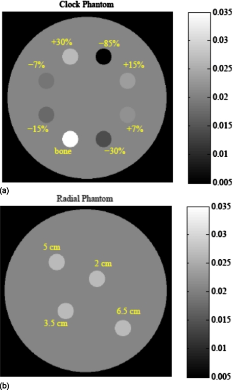
Two simulation phantoms were used in this work to investigate the tradeoff between noise and resolution (Fig. 4). Both phantoms consist of a background 20 cm diameter water cylinder and various 2 cm diameter cylindrical inserts. The water background is set to μ=0.0205 mm−1 corresponding to the 61 keV energy of our monoenergetic simulation. The main noise-resolution tradeoff comparison is made using the clock phantom, which contains eight inserts of varying contrast. Each insert center is located 5.5 cm from the image FOV center. The clock phantom allows us to investigate the effect of varying contrast magnitudes on the noise-resolution tradeoff.
Figure 4.
Simulation phantoms consist of a 20 cm water cylinder with various 2 cm diameter contrast inserts. (a) The clock phantom with eight inserts of varying contrast allows comparison of the noise-resolution tradeoff for varying magnitude of contrast. (b) The radial phantom with four inserts of the same contrast (+30%) and varying distance from the FOV center allows the spatial dependence of the noise-resolution tradeoff to be investigated.
The radial phantom contains four contrast inserts at varying radial distances from the FOV center. Inserts with the same contrast (+30%) and varying distance from the FOV center (2–6.5 cm) allow us to investigate the spatial dependence of the noise-resolution tradeoff.
Noise and resolution measurement
Noise measurement
Image noise is assessed in the water region surrounding each contrast insert. For an image reconstructed from a noisy projection data set, the image noise is the standard deviation, as a percent of the water background value, for the pixels inside the noise region of interest (ROI):
| (8) |
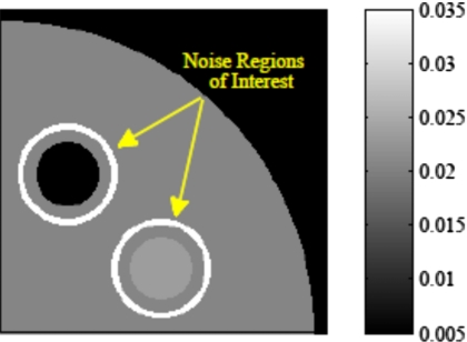
The noise ROI for each insert is an annulus that includes image pixels in the water background lying within 4–6 mm (inclusive) of the insert boundary, shown in Fig. 5, containing 756 pixels. A subtraction image between the noiseless and noisy data reconstructions is used for the variance measurement to remove systematic bias, such as sampling artifacts, from the calculation.
Figure 5.
Each insert’s annular noise region of interest consists of the 756 image pixels whose centers lie between 4 and 6 mm from the insert boundary.
To reduce computational burden, spatial statistics are used to quantify image noise in lieu of ensemble statistics. To test this, 30 monoenergetic data sets of the clock phantom, each with a different Poisson noise realization, were created and reconstructed with a single smoothing strength for each of the three algorithms. The ensemble noise in each image pixel for each algorithm was calculated from the resultant sequence of 30 images. The results of this comparison showed the use of spatial statistics within an annular ROI for noise quantification to be an adequate approximation of the average ensemble noise around each insert. The ensemble noise was seen to be slowly varying with radial distance from the FOV center, which is also shown in the radial phantom results of Sec. 3D. The dependence of noise on distance from the insert edge was found to be negligible due to the circular symmetry of the ROI and slowly varying radial dependence of the noise.
An algorithm that can reconstruct an image of comparable resolution with less noise from the same projection data offers the clinical advantage of patient dose reduction. We assume that the image noise is proportional to relative projection noise1, 24 and that projection variance is inversely proportional to the patient dose. From these assumptions, we can formulate an answer to the question “For the same image noise and resolution, how much can the AM algorithms reduce patient dose in comparison to FBP?” We calculate the dose fraction as the ratio of AM variance to FBP variance at a constant resolution metric value
| (9) |
Intuitively, the ratio of variances, or dose fraction, represents the fraction of dose necessary for the AM algorithm to achieve the same image noise as the FBP algorithm with the same resolution metric for the chosen contrast insert.
Resolution measurement
The resolution metric used in this work is based on the modulation transfer function (MTF). While x-ray transmission CT is not a shift-invariant linear system, we believe that MTF analysis as a measure of local impulse response can still provide insight into the effect of reconstruction on edge blurring. The radial phantom study was designed to investigate the spatial variation of noise and resolution for each reconstruction algorithm.
The edge-spread function (ESF) was differentiated to obtain the line-spread function (LSF) and the Fourier transform of the LSF was calculated to obtain the MTF
| (10) |
| (11) |
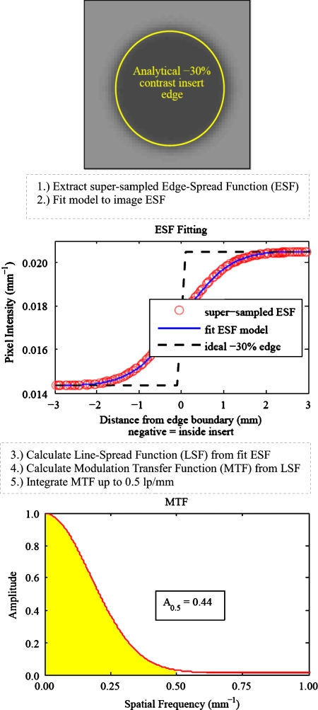
Here r is the distance between the pixel center and the known edge location. The circular symmetry of the contrast inserts can be used to construct a supersampled edge-spread function from the reconstructed image. Since our simulation phantom is comprised of a set of circular structures, we can plot each reconstructed image pixel’s intensity as a function of the distance (r) between its center and the analytically defined insert edge. As multiple pixels will have the same distance to the edge, the mean intensity at each unique distance is calculated and used for subsequent estimation of the MTF. Sampling pixels around a circularly symmetric insert to form a supersampled edge-spread function represents an average of the edge response function within the region of interest. In this way, we can view the transition between the water background and the contrast insert. This idea of using circular symmetry to oversample an edge-spread function is similar to Thornton’s use of a sphere25 to measure the in-plane MTF and slice-sensitivity profile for a multislice CT scanner. Figure 6 displays a flowchart illustrating the resolution measurement technique for the −30% contrast insert reconstructed with FBP (FWHM=2.0 mm). The location of the analytically defined insert edge is superimposed on the reconstructed image to aid visualization.
Figure 6.
Illustration of the resolution measurement for the −30% insert reconstructed using FBP with FWHM=2.0 mm.
An edge-spread function model was then fit to the supersampled ESF [ESFinsert(r)]. While the image noise is measured on images reconstructed from the noisy projection data sets, the edge-spread function is derived from images reconstructed from the noiseless projection data set to avoid bias from the image noise and to improve the model fitting. The model fitting is used to further reduce noise from the supersampled ESF prior to differentiation and Fourier transformation. Although ESFs are extracted from images reconstructed from noiseless projection data, the individual data points exhibit fluctuations due to effects such as partial volume averaging of finite voxels and the mismatch between data and reconstruction forward projectors. To avoid instability in the MTF arising from numerical differentiation of noisy data, we use an ESF model that assumes the line-spread function is well-described by a linear combination of Gaussian and exponential components26
| (12) |
| (13) |
| (14) |
The MATLAB function fminsearch is used to find the six parameters a–f that minimize the relative least-squares difference between the reconstructed image ESF and the ESF model. The second image in Fig. 6 shows the supersampled ESFinsert(r) and the fitted model. All contrast inserts within an image are fitted separately. Each fitted ESF model is then differentiated to obtain the LSF, which is then Fourier transformed to calculate the MTF for the reconstructed contrast insert of interest.
To analyze the noise-resolution tradeoff for a particular reconstruction algorithm, i.e., how the image noise and resolution vary with increasing smoothing strength, it is useful to extract a single parameter to characterize resolution for each contrast insert in each image. This will allow us to plot a curve of how the edge resolution is degraded as the image noise is reduced. La Rivière14 reported the FWHM of a Gaussian blurring model fitted to line profiles of high-contrast bone inserts. This is an intuitive metric as a wider Gaussian represents a blurrier edge. However, our six-parameter Gaussian-exponential model does not lead to such a straightforward metric.
We choose to report the area under the MTF curve up to 0.5 lp∕mm as a single-value surrogate of edge resolution. The 0.5 lp∕mm integration limit was chosen as it is near the frequency where MTF shapes differ the most between FBP and AM-700, as shown later in Fig. 7. It is also close to the ACR’s accreditation requirement of 0.6 lp∕mm for high-contrast resolution. The MTF area for a particular reconstructed insert edge is calculated as the area under the MTF up to 0.5 lp∕mm or
| (15) |
The MTF area is normalized to 0.5, as this is the area under an ideal MTF curve that has amplitude 1.0 for all spatial frequencies. Refer again to Fig. 6 for the calculated MTF and subsequent MTF area metric of an example contrast insert. Intuitively, the MTF area represents the fraction of ideal input signal that is recovered for spatial frequencies less than or equal to 0.5 lp∕mm.
Figure 7.
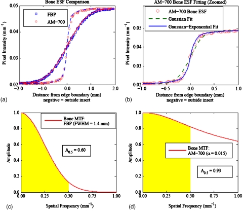
(a) Comparison of the bone insert ESF shape for the FBP algorithm with FWHM=1.4 mm and the AM-700 algorithm with α=0.015. The corresponding lines represent the Gaussian-exponential model fit used for the estimation of the MTF. Smoothing strengths were chosen for comparison as they reconstructed nearly matched image noise (∼1.09%±0.01%). Note the difference in ESF shape between the two algorithms in (a) at nearly matched image noise. The FBP edge-spread functions were found to be well fit by both Gaussian and Gaussian-exponential blurring models. (b) zooms in on the AM-700 ESF fitting to show that the Gaussian blurring model had trouble fitting the steep central transition and shoulder roll-off seen in the AM-700 high-contrast edges. This finding motivated the use of the Gaussian-exponential blurring model to fit all of the edge-spread functions in this work. (c) and (d) display the MTF calculation for the FBP and AM-700 bone inserts, respectively.
RESULTS
Necessity of Gaussian-exponential edge-spread function model
Previous investigators have characterized CT image resolution under the assumption of Gaussian blurring, e.g., the FWHM of a Gaussian ESF model14 as a surrogate for resolution. Our preliminary work revealed that purely Gaussian blurring models did not fit the AM-700 high-contrast edges well. Figure 7 illustrates the different shapes of the high-contrast bone insert ESF and subsequent calculated MTFs as reconstructed with the FBP and AM-700 algorithms. The smoothing strengths of the noiseless FBP and AM-700 edge-spread functions in Fig. 7 were chosen for comparison as they led to nearly the same image noise (∼1.09%±0.01%) when reconstructing the 100k noisy data set.
The steep central transition and shoulder roll-off of the AM-700 high-contrast edges was found to be poorly fit by a purely Gaussian blurring model [Fig. 7b] and motivated us to use the edge-spread function model [Eq. 12], which assumes the blurring kernel has both Gaussian and exponential components. The Gaussian-exponential model was used to fit all reconstructed image edge-spread functions in this work to provide a consistent methodology. No loss of ESF fitting quality with the Gaussian-exponential model was seen for the edges that were well fit by the purely Gaussian model, such as all FBP edges, all AM-100 edges, and AM-700 low-contrast (≤30%) edges.
In contrast with the FBP bone MTF [Fig. 7c], in which the amplitude quickly drops, the AM-700 bone MTF [Fig. 7d] shows an initial drop for low frequencies due to the rounded shoulder of the AM-700 ESF and retention of higher spatial frequencies due to the sharp central transition of the ESF. For high-contrast structures reconstructed by the AM-700 algorithm, the ESF and MTF shape were found to be markedly different than those seen in the literature.15, 16, 25, 27 Conventional MTF metrics, such as the spatial frequency corresponding to 10% MTF and 50% MTF, were found to provide poor characterization of the curves, given the long MTF tails of the high-contrast AM-700 structures. For example, the 10% MTF for AM-700 bone insert shown in Fig. 7d occurs at a frequency of 2.79 lp∕mm, while the corresponding FBP MTF is essentially zero at this frequency. The desire for a single-valued metric that describes a clinically relevant feature common to all the MTF shapes characteristic of our study motivated our use of the MTF area as a surrogate for resolution.
Noise-resolution tradeoff for varying contrast
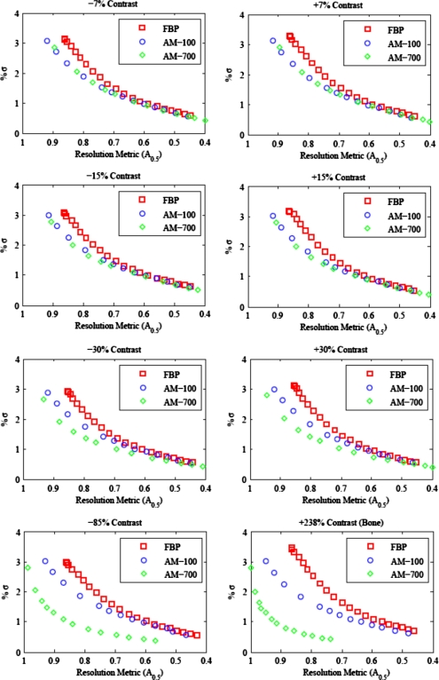
For each reconstructed clock phantom image, the relative noise in the water background and the MTF area were determined independently for each of the eight contrast inserts. Plotting the image noise as a function of resolution (MTF area) for a set of images reconstructed by a particular algorithm with varying levels of smoothing strength describes the noise-resolution tradeoff characteristic of the algorithm.
Figure 8 compares the noise-resolution tradeoff between the FBP algorithm and the AM algorithm, with δ=100 and δ=700 for images reconstructed from the 100k noisy projection data. The tradeoff curves for the clock phantom’s eight contrast inserts are plotted separately to show how the tradeoff varies with the magnitude of contrast. Each point along a curve represents an image with a unique smoothing strength. For display purposes, the unpenalized AM images are not included on the AM tradeoff curves as the image noise is greater than 6% and reduces the scale of the noise axis. The noise in the water background around each contrast insert within a single reconstructed image is essentially the same. Thus, the differences seen in the AM tradeoff curves for varying magnitudes of insert contrast are due to differences in the resolution. This is a direct result of the nonquadratic local neighborhood penalty function. Also, note that the FBP algorithm appears to have a lower achievable resolution than AM; this is a result of the raised cosine roll-off windowed ramp function used for FBP in this work.
Figure 8.
Noise-resolution tradeoff curves for the clock phantom reconstructed with 100k projection noise. Note the reverse x-axis. As the smoothing strength is increased, noise is reduced at the cost of reduced resolution. The tradeoff curve for AM with δ=700 for the penalty function is markedly different for structures of varying contrast.
For all magnitudes of contrast, the AM tradeoff curves lie below the FBP algorithm curve. Both AM-100 and AM-700 reconstruct images with either less image noise for the same resolution metric, sharper edges for matched image noise or, by extension, images with similar resolution and image noise for less patient dose. The AM-700 algorithm shows an increasing benefit as the contrast magnitude used for resolution comparison is increased. The clock phantom study shows us that the noise-resolution tradeoff advantage of the penalized AM algorithm in comparison with conventional FBP is dependent on the contrast magnitude used for resolution calculation and the choice of parameter value for AM’s edge-preserving penalty function.
Effect of projection noise magnitude
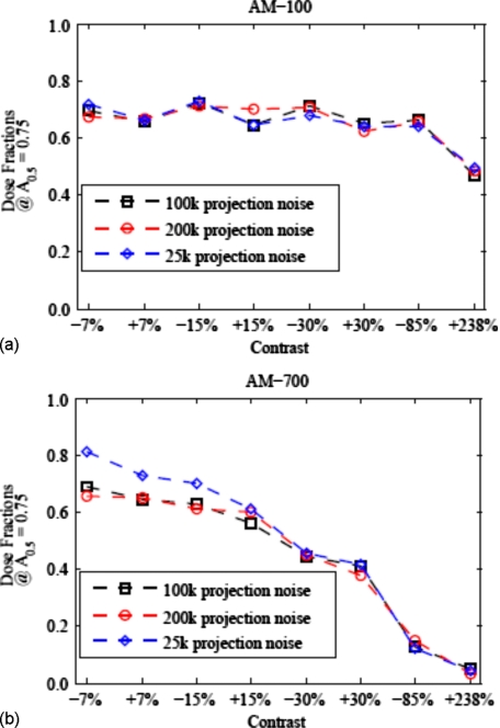
As outlined in Sec. 2C1, the potential for dose reduction that the AM algorithm offers is calculated as the ratio of AM-insert variance to FBP-insert variance when matching the resolution metric for a chosen contrast insert. By applying spline interpolation to the tradeoff curves of Fig. 8, FBP and AM noise levels for a matched resolution metric of A0.5=0.75 were estimated. The resulting AM-to-FBP variance ratio (for all three projection noise realizations) is plotted as a function of contrast in Fig. 9. The magnitude of projection noise investigated in the three noise realizations does not appear to have a marked effect on the advantage of the AM algorithm. The maximum impact of low dose (25k) and low noise (200k) imaging techniques relative to 100k is seen for the AM-700 low-contrast structures ranging from 0.66 to 0.81 [Fig. 9b]. This variation was overshadowed by the variation due to contrast magnitude for the AM-700 algorithm, for which the variance ratio ranges from 0.69 to 0.05 (100k projection noise realization). Figure 9 shows that the potential for dose reduction is largely driven by the contrast magnitude chosen for matching image resolution.
Figure 9.
AM/FBP variance ratio at a matched resolution value of AMTF0.5=0.75 for each of the eight inserts of the clock phantom. (a) and (b) display the results for AM-100 and AM-700, respectively. The 100k projection noise case is plotted as the baseline with the low noise (200k) and low dose (25k) cases plotted for comparison. As can be seen, the three noise realizations cause some variability in the dose fractions, but this is overshadowed by the choice of penalty function parameter values and contrast magnitude effects.
Spatial dependence of noise-resolution tradeoff
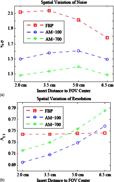
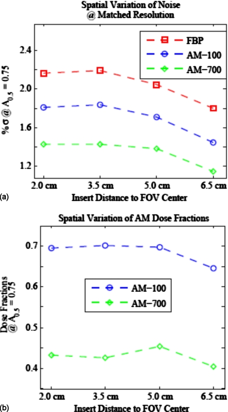
The dependence of resolution, noise, and variance ratio on spatial location is illustrated in Figs. 1011. Within a single reconstructed image, FBP noise varies more with FOV location than the AM image noise [Fig. 10a]. In contrast, Fig. 10b shows that AM resolution increases with distance from the FOV center, while FBP resolution is nearly spatially constant. Figure 11 shows the spatial variation of noise and variance ratios for AM and FBP images with a matched spatial resolution metric of A0.5=0.75. For all algorithms, resolution-matched image noise decreases with increasing distance from the FOV center. This is not surprising, as the projection noise for the peripheral insert locations is smaller due to a shorter average path length through the phantom for the source-detector rays that traverse the peripheral image pixels. The dose fraction of the AM algorithm is nearly the same for all four insert locations [Fig. 11b] with dose fractions ranging from 0.65 to 0.70 for AM-100 and from 0.41 to 0.45 for AM-700.
Figure 10.
Results of the radial phantom study showing the spatial dependence of (a) noise and (b) resolution within a single reconstructed image from each algorithm. The smoothing strengths were chosen such that the resolution metric for the reconstruction algorithms were similar for purposes of comparison. The AM resolution increases with distance from the FOV center, while the FBP algorithm’s resolution does not. FBP image noise varies more spatially than for the AM algorithm.
Figure 11.
Comparison of the noise-resolution tradeoff for varying distance from FOV center. When compared at matched resolution (noise interpolated to matched A0.5=0.75), (a) the FBP and AM algorithms show similar variation of noise across the FOV and (b) the dose fraction stays nearly constant for all inserts.
Reconstructed image comparison
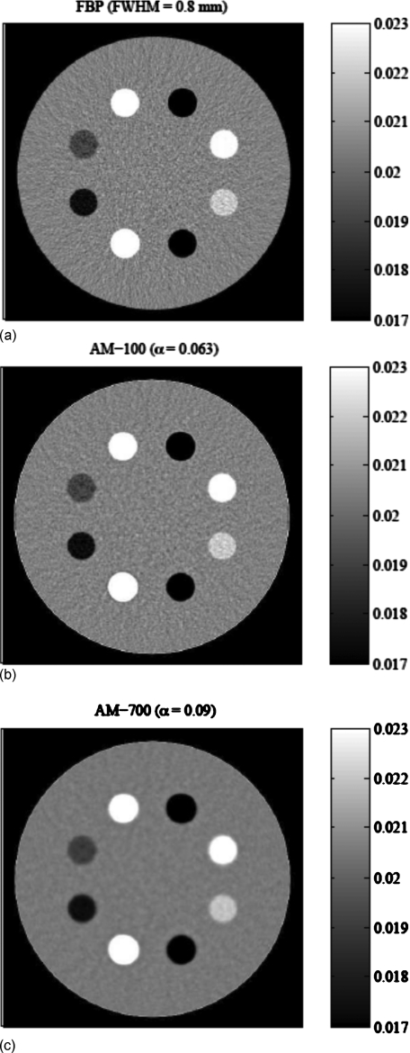
Figure 12 shows images of the simulated clock phantom reconstructed from the 100k noisy data set with similar resolutions (A0.5∼0.75) around the high-contrast bone insert. The AM-700 image noise level is only 25% of that of the FBP image. While the AM-700 high-contrast resolution metric value nearly matches that of the FBP images, the low-contrast inserts exhibit subjectively poorer resolution than that of the FBP algorithm. In comparison, the AM-100 algorithm was found to offer comparable resolution to the FBP for all contrast inserts, with about 70% of the noise relative to FBP.
Figure 12.
Reconstructed images of the simulated clock phantom data with nearly matched bone insert (7 o’clock position) resolution metric of A0.5∼0.75. All images set to identical ±15% window [0.017:0.023] mm−1 for display of image noise. Noise around the bone insert is (a) 2.04% for FBP, (b) 1.36% for AM-100, and (c) 0.47% for AM-700.
Note the presence of an artifact around the phantom edge in the AM images [Figs. 12b, 12c]. The literature9, 28 has shown these artifacts are in fact inherent to maximum likelihood reconstruction methods and arise from mismatches between the SIR algorithm’s forward model and the true physical detection process. Zbijewski28 shows that reconstructing on a finer voxel grid alleviates much of the edge artifact, but this will lead to much longer computing times. While the smallest penalty strength (αmin) was found to eliminate the edge artifact around the internal contrast inserts for both AM-100 and AM-700, further work will be needed to address the ringing artifact around the phantom edge if it is determined to be of clinical concern.
Qualitative real data comparison
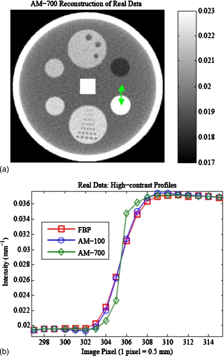
Real CT data includes effects from physical phenomena such as beam-hardening and scatter, which are known to degrade image quality. Figure 13 illustrates the ability of the penalized AM algorithm to reconstruct images from axial sinograms acquired on the Philips Brilliance Big Bore scanner. Smoothing strengths for the three reconstructions were tuned to give nearly the same noise in a 2×2 cm2 square ROI (1600 total pixels) in the center of the water region. For the low-contrast detectability insert (6 o’clock) differences among the three reconstructions could not be visually discerned. However, profiles through the high-contrast insert, located at 4 o’clock, reveal sharper edge discrimination for the AM-700 algorithm [Fig. 13b], which motivates future work to investigate the noise-resolution tradeoff using real CT data.
Figure 13.
(a) AM-700 reconstructed image of the multipin layer of a daily QA phantom from real data acquired on a Philips Brilliance Big Bore CT scanner. Smoothing strengths were adjusted to match noise (∼0.94% in the central square ROI) within 0.005% among the AM-700, AM-100, and FBP images. (b) Visible differences in the high-contrast insert (4 o’clock) are illustrated in the profiles.
DISCUSSION
This work compares the noise-resolution tradeoff of the conventional filtered backprojection algorithm to that of the alternating minimization algorithm with two different parameter values for a local edge-preserving penalty function. This is not the first work comparing the noise-resolution tradeoff between filtered backprojection and statistical iterative algorithms. However, it is the first to do so for the alternating minimization algorithm for x-ray transmission tomography, which supports an exact solution to the maximization of the Poisson log-likelihood (M-step). The conclusions from the simulation study presented here could reasonably be extrapolated to other SIR algorithms that seek to maximize the same penalized-likelihood objective function, since the AM solution images are very near complete convergence due to the large number of iterations employed. It is also the first, to the best of the authors’ knowledge, to characterize the noise-resolution tradeoff curves and subsequent dose-reduction factors for a range of contrast magnitudes.
In this paper, we selected the normalized MTF integral up to a cutoff frequency of 0.5 lp∕mm as a convenient, but somewhat arbitrary, single-parameter metric for quantifying spatial resolution. Other integration limits up to the Nyquist frequency were considered but were found to increase the reported AM-700 advantage due to AM-700’s longer MTF tails for high-contrast structures. For comparing FBP and AM resolution, the 0.5 lp∕mm limit was chosen to ensure significant overlap of the nonzero frequency content of the corresponding MTFs, which potentially have very different shapes and high-frequency tails. This limit was considered to be a conservative choice for reporting dose-reduction potential. While in theory the MTF is a linear-systems metric and CT resolution is known to be spatially variant over the FOV,29 we believe that a MTF derived from a supersampled edge-spread function objectively describes the spatial frequency content in the local region. The concept of measuring the MTF for structures within a CT image dates back three decades27 and is still a topic of debate to this day. To the author’s knowledge, no gold standard metric for quantifying CT image resolution has been embraced by the community, making direct comparison of our results and other works difficult.
Not surprisingly, the log-cosh penalized alternating minimization algorithm, which models detector counting statistics, reconstructs images with less noise than conventional filtered backprojection images of comparable resolution. In contrast with other investigations that matched high-contrast structure resolution, e.g., bone and steel beads, our study shows that the noise-resolution tradeoff for nonquadratic neighborhood penalty functions markedly varies with contrast magnitude of the edge used for quantifying resolution. The apparent advantage of using the log-cosh penalized AM algorithm when comparing high-contrast resolution was found to be moderately to substantially diminished when the resolutions of low-contrast edges were compared. Moreover, this variation was found to strongly depend on the chosen penalty function parameters.
Despite some loss of benefit for low-contrast objects, the ratio of variances for high-contrast objects in this work implies that the penalized AM algorithm is capable of reconstructing images with comparable quality to FBP using 10%–70% of the dose required by FBP, depending on the penalty function parameters (Fig. 9). This is compatible with the growing clinical literature; Stayman30 reported SIR-to-FBP image SNR ratios of about 1.6 for a PET system. For x-ray transmission CT, Ziegler15 reported SIR-to-FBP noise ratios of 2.1 to 3.0, implying dose-reduction factors of 4.4 to 9.0. La Rivière14 described an expectation-maximization sinogram smoothing technique which achieved a noise-resolution tradeoff similar to the adaptive trimmed mean filter approach2 that uses 50% less dose. These studies exhibit a range of dose-reduction factors for a number of reasons. Since the dose-reduction factor is a ratio of variances at an arbitrary value of the resolution metric, choosing a different value of the resolution metric along the noise-resolution tradeoff curve for matching will change the reported variance ratios. In addition, there are differences between the SIR and the FBP reconstruction algorithms used in the literature and the metrics used to quantify resolution. In spite of these differences, our reported dose-reduction potentials for high-contrast structures are in reasonable agreement with the published literature.
Varying the magnitude of noise in the projection data was found to only minimally affect the variance ratio at a matched spatial resolution in our simulations (Fig. 9). In contrast, Ziegler et al.15 showed that projection noise level does affect the SIR-to-FBP noise ratio. His work further showed that this effect was stronger for points farther from the FOV center than those near the center. Our range of distances from the FOV center (2–6.5 cm) was much smaller than those in Ziegler’s work (1.5–20 cm). We found the contrast magnitude and penalty parameter choice to have a greater effect on the variance ratio than projection noise.
As our work utilized a spatially invariant penalty function, it would be expected that AM images exhibit spatially variant and anisotropic resolution.29 Our study of the radial phantom shows that the resolution and noise vary differently with distance from the FOV center of AM and FBP images (Fig. 10). In contrast with studies that report FBP resolution to degrade with increasing distance,15 the FBP algorithm in this work showed little spatial variation of resolution. This difference could stem from slight differences in the FBP algorithm or the larger range of distances to FOV center that Ziegler investigated. The variation of AM resolution with distance from the FOV center [Fig. 10b] illustrates the nonuniform nature of the AM resolution. Interestingly, we found the AM-to-FBP variance ratio for a fixed resolution to be approximately constant over the FOV (Fig. 11).
Resolution anisotropy was studied by separating the total annular ROIs around the insert edges in the radial phantom into four Cartesian quadrants and calculating the associated MTFs using the same procedure described above. The quadrant MTFs in the FBP image were found to vary little from the MTF of the total ROI. The penalized AM quadrant MTFs were found to vary from one another, especially in the tangential and radial directions, indicative of anisotropic resolution. The AM anisotropies were found to be small compared to the differences between the AM and FBP algorithms, perhaps in part due to the highly symmetric nature of the phantoms investigated here. The resolution metric calculated from the total annular ROI represents an average of the local resolution in the region surrounding each contrast insert.
Methods for designing spatially variant quadratic penalty functions that achieve a target response have been described in the literature and shown to support nearly uniform and isotropic resolution for PET and transmission x-ray CT problems.30, 31, 32 Ahn and Leahy33 reported on the design of nonquadratic regularization penalties with similar goals in PET.33 Design of penalty functions, both quadratic and nonquadratic, that include the ideas of spatially variant29 and nonlocal penalty functions20 to achieve desirable properties such as uniform, isotropic resolution are important areas of ongoing work for x-ray transmission CT.
The quantitative results presented in this work have been performed exclusively in an idealized 2D x-ray CT simulation environment, with projection noise assumed to follow the simple Poisson distribution. While this data model allows detection of very subtle effects of reconstruction algorithm on noise-resolution tradeoffs, obviously clinical translation requires handling complex detector nonlinearities and nonideal behaviors. Both the AM (Ref. 13) and parabolic surrogates34 SIR algorithms generalize to more complex data models which include polyenergetic spectra, scatter, and correlated noise, all of which are necessary to extract statistically optimal smoothed images from measured sinogram data. SIR algorithms including the known polyenergetic x-ray spectrum in their forward model have been shown to outperform FBP reconstruction preceded by sinogram linearization corrections in terms of nonuniformity from beam-hardening artifacts.35 Our example clinical case (Fig. 13) suggests (but by no means proves) that our main conclusions are preserved, at least qualitatively, in the transition to more realistic data models. Beam-hardening and scatter effects manifest themselves as artifacts, i.e., systematic shifts in the mean image intensities. While such streaking and nonuniformity artifacts caused by these data mismatches play a large role in subjective image quality and quantitative CT, we would not expect these nonlinear processes to substantially affect the spatial resolution-noise tradeoff characteristic of the device. The logical next step in translating AM benefits to quantitative CT imaging to the clinic is to repeat systematic studies of resolution-noise tradeoff using more realistic data models and experimentally acquired data sets derived from scanning phantoms of known geometry and composition. Another issue is the incorporation of 3D system geometry (spiral multirow detector geometry) into the forward SIR projector. 3D SIR algorithms have been shown to alleviate CBCT artifacts, e.g., incomplete data artifacts in off-axis planes) characteristic of conventional FBP reconstruction.17 However, the Shi and Fessler36 design of three-dimensional penalty functions pose challenges, providing another important area of future investigation.
Long SIR computing times constitute another barrier to widespread clinical acceptance. Recent literature describing GE’s adaptive statistical iterative reconstruction (ASIR) algorithm shows that simplified statistical algorithms can still provide diagnostically viable images with 50% or 65% smaller doses than needed for conventional FBP.37, 38, 39 While the ASIR algorithm does not include modeling of the system matrix, which can play a large role in reducing artifacts and noise,16, 17 trained observers have rated the ASIR images acquired at 50% of the FBP dose to have similar, if not better, image quality for almost all metrics studied. The literature has shown that the simplified ASIR algorithm has the capability to reconstruct image volumes acceptable to current trained observers in a clinically relevant timeframe of 65 s compared to 50 s for FBP.39 For the AM algorithm, Keesing et al.40, 41 has demonstrated the feasibility of speeding up the computation time by parallelizing the projection operations for a fully 3D helical geometry.
Comparing the AM-100 and AM-700 results reveals the importance of optimizing the nonquadratic penalty function parameter δ. AM-700, with a penalty that transitions to linear growth for smaller pixel differences, shows greatly improved noise performance over AM-100 and the FBP algorithm when comparing high-contrast resolution. However, when comparing images with nearly matched high-contrast resolution metric values, AM-700 was seen to have worse resolution for the low-contrast inserts. The log-cosh penalty function with δ=700 could be beneficial where high-contrast resolution is important and reduced low-contrast resolution is acceptable, e.g., for dose reduction in image registration applications using bony landmarks. For clinical situations in which low-contrast resolution is important, for example, intensity-driven soft-tissue deformable image registration or soft-tissue delineation for contouring, log-cosh penalized AM with δ=100 could provide comparable image quality with 70% of the FBP dose. The results presented here show the need for future work in penalty function parameter optimization and those choices will certainly be task-specific.42
CONCLUSIONS
This work assessed the noise-resolution tradeoff of the penalized alternating minimization algorithm in comparison with FBP for a set of structures with a range of contrast magnitudes (±7% to +238%) and varying distance from the FOV center (2–6.5 cm). An idealized simulation environment was used to isolate the effects of each algorithm’s smoothing technique. A spatial resolution metric A0.5, derived from ESFs in the reconstructed image, was developed in response to the observation that the AM-700 MTF shape for high-contrast edges deviates significantly from that of FBP images. The parameter value used to specify AM’s local log-cosh penalty function has been shown to drastically modulate noise-resolution tradeoff curves and subsequent dose-reduction potentials reported for SIR algorithms. The noise-resolution tradeoff was also found to be greatly affected by the contrast of the structure used for evaluating spatial resolution. The range of projection noise levels investigated here and the variation in structure distance from FOV center only minimally affected the noise-resolution tradeoff. The ratio of AM-to-FBP image variance ratio for matched resolution surrogate implies a dose-reduction potential; the AM algorithm has the potential to reconstruct images with comparable noise and MTF area using only 10%–70% of the FBP dose. These values are in line with other published literature. The result that log-cosh penalized AM noise-resolution tradeoff is dependent on the contrast magnitude implies that nonquadratic penalty function parameters can be optimized to maximize the dose-reduction potential for specific imaging tasks.
ACKNOWLEDGMENTS
This work was supported in part from Grant Nos. R01 CA 75371, P01 CA 116602, and 5P30 CA 016059 awarded by the National Institutes of Health.
References
- Kak A. C. and Slaney M., Principles of Computerized Tomographic Imaging (IEEE, New York, 1988). [Google Scholar]
- Hsieh J., “Adaptive streak artifact reduction in computed tomography resulting from excessive x-ray photon noise,” Med. Phys. 25(11), 2139–2147 (1998). 10.1118/1.598410 [DOI] [PubMed] [Google Scholar]
- Endo M., Tsunoo T., Nakamori N., and Yoshida K., “Effect of scattered radiation on image noise in cone beam CT,” Med. Phys. 28(4), 469–474 (2001). 10.1118/1.1357457 [DOI] [PubMed] [Google Scholar]
- Joseph P. M. and Spital R. D., “The effects of scatter in x-ray computed tomography,” Med. Phys. 9(4), 464–472 (1982). 10.1118/1.595111 [DOI] [PubMed] [Google Scholar]
- Joseph P. M. and Spital R. D., “A method for correcting bone induced artifacts in computed tomography scanners,” J. Comput. Assist. Tomogr. 2(1), 100–108 (1978). 10.1097/00004728-197801000-00017 [DOI] [PubMed] [Google Scholar]
- Joseph P. M. and Spital R. D., “The exponential edge-gradient effect in x-ray computed tomography,” Phys. Med. Biol. 26(3), 473–487 (1981). 10.1088/0031-9155/26/3/010 [DOI] [PubMed] [Google Scholar]
- Lange K. and Carson R., “EM reconstruction algorithms for emission and transmission tomography,” J. Comput. Assist. Tomogr. 8(2), 306–316 (1984). [PubMed] [Google Scholar]
- Fessler J. A., “Statistical image reconstruction methods for transmission tomography,” in Medical Image Processing and Analysis, Handbook of Medical Imaging, Vol. 2, edited by Sonka M. and Fitzpatrick J. M. (SPIE, Bellingham, 2000), pp. 1–70. [Google Scholar]
- Snyder D. L., Miller M. I., Thomas L. J., and Politte D. G., “Noise and edge artifacts in maximum-likelihood reconstructions for emission tomography,” IEEE Trans. Med. Imaging 6(3), 228–238 (1987). 10.1109/TMI.1987.4307831 [DOI] [PubMed] [Google Scholar]
- Byrne C. L., “Iterative image reconstruction algorithms based on cross-entropy minimization,” IEEE Trans. Image Process. 2(1), 96–103 (1993). 10.1109/83.210869 [DOI] [PubMed] [Google Scholar]
- Brenner D. J. and Hall E. J., “Computed tomography—An increasing source of radiation exposure,” N. Engl. J. Med. 357(22), 2277–2284 (2007). 10.1056/NEJMra072149 [DOI] [PubMed] [Google Scholar]
- Williamson J. F., Li S., Devic S., Whiting B. R., and Lerma F. A., “On two-parameter models of photon cross sections: Application to dual-energy CT imaging,” Med. Phys. 33(11), 4115–4129 (2006). 10.1118/1.2349688 [DOI] [PubMed] [Google Scholar]
- O’Sullivan J. A. and Benac J., “Alternating minimization algorithms for transmission tomography,” IEEE Trans. Med. Imaging 26(3), 283–297 (2007). 10.1109/TMI.2006.886806 [DOI] [PubMed] [Google Scholar]
- La Rivière P. J., “Penalized-likelihood sinogram smoothing for low-dose CT,” Med. Phys. 32(6), 1676–1683 (2005). 10.1118/1.1915015 [DOI] [PubMed] [Google Scholar]
- Ziegler A., Kohler T., and Proksa R., “Noise and resolution in images reconstructed with FBP and OSC algorithms for CT,” Med. Phys. 34(2), 585–598 (2007). 10.1118/1.2409481 [DOI] [PubMed] [Google Scholar]
- Sunnegårdh J. and Danielsson P. E., “Regularized iterative weighted filtered backprojection for helical cone-beam CT,” Med. Phys. 35(9), 4173–4185 (2008). 10.1118/1.2966353 [DOI] [PubMed] [Google Scholar]
- Thibault J. B., Sauer K. D., Bouman C. A., and Hsieh J., “A three-dimensional statistical approach to improved image quality for multislice helical CT,” Med. Phys. 34(11), 4526–4444 (2007). 10.1118/1.2789499 [DOI] [PubMed] [Google Scholar]
- Csiszar I., “Why least squares and maximum entropy? An axiomatic approach to inference for linear inverse problems,” Ann. Stat. 19, 2032–2066 (1991). 10.1214/aos/1176348385 [DOI] [Google Scholar]
- Green P. J., “Bayesian reconstructions from emission tomography data using a modified EM algorithm,” IEEE Trans. Med. Imaging 9(1), 84–93 (1990). 10.1109/42.52985 [DOI] [PubMed] [Google Scholar]
- Yu D. F. and Fessler J. A., “Edge-preserving tomographic reconstruction with nonlocal regularization,” IEEE Trans. Med. Imaging 21(2), 159–173 (2002). 10.1109/42.993134 [DOI] [PubMed] [Google Scholar]
- Hudson H. M. and Larkin R. S., “Accelerated image reconstruction using ordered subsets of projection data,” IEEE Trans. Med. Imaging 13(4), 601–609 (1994). 10.1109/42.363108 [DOI] [PubMed] [Google Scholar]
- Whiting B. R., Massoumzadeh P., Earl O. A., O’Sullivan J. A., Snyder D. L., and Williamson J. F., “Properties of preprocessed sinogram data in x-ray computed tomography,” Med. Phys. 33(9), 3290–3303 (2006). 10.1118/1.2230762 [DOI] [PubMed] [Google Scholar]
- Lasio G. M., Whiting B. R., and Williamson J. F., “Statistical reconstruction for x-ray computed tomography using energy-integrating detectors,” Phys. Med. Biol. 52(8), 2247–2266 (2007). 10.1088/0031-9155/52/8/014 [DOI] [PubMed] [Google Scholar]
- Chesler D., Riederer S., and Pelc N., “Noise due to photon counting statistics in computed x-ray tomography,” J. Comput. Assist. Tomogr. 1(1), 64–74 (1977). 10.1097/00004728-197701000-00009 [DOI] [PubMed] [Google Scholar]
- Thornton M. M. and Flynn M. J., “Measurement of the spatial resolution of a clinical volumetric computed tomography scanner using a sphere phantom,” Proc. SPIE 6142, 707–716 (2006). [Google Scholar]
- Boone J. M. and Seibert J. A., “An analytical edge spread function model for computer fitting and subsequent calculation of the LSF and MTF,” Med. Phys. 21(10), 1541–1545 (1994). 10.1118/1.597264 [DOI] [PubMed] [Google Scholar]
- Judy P. F., “The line spread function and modulation transfer function of a computed tomographic scanner,” Med. Phys. 3(4), 233–236 (1976). 10.1118/1.594283 [DOI] [PubMed] [Google Scholar]
- Zbijewski W. and Beekman F. J., “Characterization and suppression of edge and aliasing artefacts in iterative x-ray CT reconstruction,” Phys. Med. Biol. 49(1), 145–157 (2004). 10.1088/0031-9155/49/1/010 [DOI] [PubMed] [Google Scholar]
- Fessler J. A. and Rogers W. L., “Spatial resolution properties of penalized-likelihood image reconstruction: Space-invariant tomographs,” IEEE Trans. Image Process. 5(9), 1346–1358 (1996). 10.1109/83.535846 [DOI] [PubMed] [Google Scholar]
- Stayman J. W. and Fessler J. A., “Compensation for nonuniform resolution using penalized-likelihood reconstruction in space-variant imaging systems,” IEEE Trans. Med. Imaging 23(3), 269–284 (2004). 10.1109/TMI.2003.823063 [DOI] [PubMed] [Google Scholar]
- Shi H. R. and Fessler J. A., “Quadratic regularization design for 2-D CT,” IEEE Trans. Med. Imaging 28(5), 645–656 (2009). 10.1109/TMI.2008.2007366 [DOI] [PMC free article] [PubMed] [Google Scholar]
- Stayman J. W. and Fessler J. A., “Regularization for uniform spatial resolution properties in penalized-likelihood image reconstruction,” IEEE Trans. Med. Imaging 19(6), 601–615 (2000). 10.1109/42.870666 [DOI] [PubMed] [Google Scholar]
- Ahn S. and Leahy R. M., “Analysis of resolution and noise properties of nonquadratically regularized image reconstruction methods for PET,” IEEE Trans. Med. Imaging 27(3), 413–424 (2008). 10.1109/TMI.2007.911549 [DOI] [PubMed] [Google Scholar]
- Lange K. and Fessler J. A., “Globally convergent algorithms for maximum a posteriori transmission tomography,” IEEE Trans. Image Process. 4(10), 1430–1438 (1995). 10.1109/83.465107 [DOI] [PubMed] [Google Scholar]
- Yan C. H., Whalen R. T., Beaupre G. S., Yen S. Y., and Napel S., “Reconstruction algorithm for polychromatic CT imaging: Application to beam hardening correction,” IEEE Trans. Med. Imaging 19(1), 1–11 (2000). 10.1109/42.832955 [DOI] [PubMed] [Google Scholar]
- Shi H. R. and Fessler J. A., “Quadratic regularization design for iterative reconstruction in 3D multi-slice axial CT,” in Proceedings of the IEEE Nuclear Science Symposium, 2006. (unpublished).
- Hara A. K., Paden R. G., Silva A. C., Kujak J. L., Lawder H. J., and Pavlicek W., “Iterative reconstruction technique for reducing body radiation dose at CT: Feasibility study,” AJR, Am. J. Roentgenol. 193(3), 764–771 (2009). 10.2214/AJR.09.2397 [DOI] [PubMed] [Google Scholar]
- Prakash P., Kalra M. K., Kambadakone A. K., Pien H., Hsieh J., Blake M. A., and Sahani D. V., “Reducing abdominal CT radiation dose with adaptive statistical iterative reconstruction technique,” Invest. Radiol. 45(4), 202–210 (2010). 10.1097/RLI.ob013e3181dzfeec [DOI] [PubMed] [Google Scholar]
- Silva A. C., Lawder H. J., Hara A., Kujak J., and Pavlicek W., “Innovations in CT dose reduction strategy: Application of the adaptive statistical iterative reconstruction algorithm,” AJR, Am. J. Roentgenol. 194(1), 191–199 (2010). 10.2214/AJR.09.2953 [DOI] [PubMed] [Google Scholar]
- Keesing D. B., O’Sullivan J. A., Politte D. G., and Whiting B. R., “Parallelization of a fully 3D CT iterative reconstruction algorithm,” in Proceedings of the IEEE International Symposium on Biomedical Imaging, pp. 1240–1243, 2006. (unpublished).
- Keesing D. B., O’Sullivan J. A., Politte D. G., Whiting B. R., and Snyder D. L., “Missing data estimation for fully 3D spiral CT image reconstruction,” in Proceedings of SPIE: Medical Imaging 2007: Physics of Medical Imaging, San Diego, CA, 2007. (unpublished).
- Sprawls P., “AAPM tutorial. CT image detail and noise,” Radiographics 12(5), 1041–1046 (1992). [DOI] [PubMed] [Google Scholar]


