EpiChIP: gene-by-gene quantification of epigenetic modification levels

Abstract

The combination of chromatin immunoprecipitation with next-generation sequencing technology (ChIP-seq) is a powerful and increasingly popular method for mapping protein–DNA interactions in a genome-wide fashion. The conventional way of analyzing this data is to identify sequencing peaks along the chromosomes that are significantly higher than the read background. For histone modifications and other epigenetic marks, it is often preferable to find a characteristic region of enrichment in sequencing reads relative to gene annotations. For instance, many histone modifications are typically enriched around transcription start sites. Calculating the optimal window that describes this enrichment allows one to quantify modification levels for each individual gene. Using data sets for the H3K9/14ac histone modification in Th cells and an accompanying IgG control, we present an analysis strategy that alternates between single gene and global data distribution levels and allows a clear distinction between experimental background and signal. Curve fitting permits false discovery rate-based classification of genes as modified versus unmodified. We have developed a software package called EpiChIP that carries out this type of analysis, including integration with and visualization of gene expression data.

INTRODUCTION

A major goal of molecular biology is to understand how the complex patterns of gene expression that define cell types and states are organized and maintained. An important step towards this aim is the positional mapping of DNA-interacting proteins, such as transcription factors (TFs), histones or basic transcriptional machinery on chromosomes. Linking this information to the expression levels of genes provides important insights into the regulation of transcription.

The main experimental strategy for studying protein–DNA interaction in vivo is chromatin immunoprecipitation (ChIP) (1), which is based on antibody-mediated enrichment of protein–DNA complexes. Hybridization of the immunoprecipitated DNA to tiling or promoter microarrays (ChIP-chip) allowed extension of ChIP from single-gene studies to the whole genome (2). A breakthrough for ChIP-based assays came with the introduction of next-generation sequencing technology, such as ABI SOLiD, Roche 454, HeliScope or the Illumina Genome Analyzer (3). Mapping of the sequencing reads to the genome reveals positions where high numbers of reads pile up to create peaks, indicating protein binding sites. This approach was termed ChIP-seq and offers tremendous advantages over ChIP-chip, such as single-base pair resolution, much lower starting material requirements and the absence of DNA-hybridization-related sensitivity issues (4). ChIP-seq has therefore become the state-of-the-art technology for mapping protein–DNA interactions in a genome-wide fashion.

One of the key findings of pioneering ChIP-seq experiments for TFs such as Stat1 (5) or Rest (NRSF) (6) was the unexpectedly large number of putative binding sites that are dispersed throughout the genome. Peaks are often located far from loci or do not contain binding motifs and yet are clearly not artifactual (7). Because of this, accurate target gene assignment is currently one of the major problems with TF ChIP-seq (7). In that respect, ChIP-seq experiments for post-translational modifications on histones have been more informative. Different types of histone modifications exhibit clear patterns of distribution along the genome and were found to be associated with other functional features. For instance, trimethylation of K4 on histone H3 (H3K4me3) is primarily found at transcriptional start sites of active genes (8,9). H3K27me3 marks, on the other hand, are more spread out along the bodies of transcriptionally repressed genes (8,10). Another type of histone marks, H3K36me3, appears to mark gene bodies and particularly exons of expressed transcripts (11–13).

Because this is a common feature of histone modifications, we have developed a search strategy to identify consistent regions of genes that are globally most enriched in a given ChIP-seq data set. To date, there is a small number of published programs or packages [e.g. CEAS (14), Repitools (15)] that allow one to search for such regions.

Our approach goes further by extracting the ChIP-seq signal in this fixed window for each gene. The global distribution of this data shows a clear distinction between experimental background and signal, which we use for false discovery rate (FDR)-based classification of genes. This allows us to define which genes are significantly modified above background, and to quantify the level of modification of each individual gene.

Using H3K9/14ac in Th2 cells as an example, we illustrate this strategy for analysis of ChIP-seq data and present the software package EpiChIP, which allows one to perform this analysis in a user-friendly way.

MATERIALS AND METHODS

Th2 cell differentiation culture

Spleens of C57BL/6 mice aged from 7 weeks to 4 months were removed and softly homogenized through a nylon mesh. The medium used throughout the cell cultures was IMDM supplemented with 10% FCS, 2 µM l-glutamine, penicillin, streptomycin and 50 µM β-mercaptoethanol. Cells were washed twice and purified by a Ficoll density gradient centrifugation. Cd4+Sell+ cells were isolated by a two-step MACS purification using the naive T Cell Isolation Kit II (Miltenyi Biotec). Cells were seeded into 24-well plates that had been coated with a mix of anti-Cd3 (1 µg/ml, clone 145-2C11, eBioscience) and anti-Cd28 (5 µg/ml, clone 37.51, eBioscience) antibodies overnight, at a density of 250 000 cells/ml and a total volume of 2 ml. The following cytokines and antibodies, respectively, were added to the Th2 culture: recombinant murine Il4 (10 ng/ml, R&D Systems), neutralizing Interferon-γ (5 µg/ml, Sigma). Cells were cultured for 4–5 days at 37°C, 5% CO₂. After this, cells were taken away from the activation stimulus, diluted 1:2 in fresh medium containing the same cytokine concentration as before. After 2–3 days of resting time, cells were directly cross-linked in formaldehyde for preparing ChIP-seq samples. For FACS staining, cells were restimulated with phorbol dibutyrate and ionomycin (both used at 500 ng/ml, both from Sigma) for 4 h in the presence of Monensin (2 µM, eBioscience) for the last 2 h after the resting phase. For real-time PCRs, the cells were lysed in Trizol. FACS staining and real-time PCR showed successful Th2 differentiation (Supplementary Figure S1A and S1B).

FACS staining

After restimulation, cells were washed in PBS and fixed overnight in IC fixation buffer (eBioscience). Staining for intracellular cytokine expression was carried out according to the eBioscience protocol, using Permeabilization buffer (eBioscience), and the following antibodies: anti-Interferon-γ-APC (1/1200, clone XMG1.2, eBioscience), anti-Il13-PE (1/400, clone eBio13A, eBioscience) and anti-Gata3-Alexa647 (one test, TWAJ, eBioscience). Stained cells were analyzed on a FACSCalibur (BD Biosciences) flow cytometer using Cellquest Pro and FlowJo software.

Real-time PCR

In parallel to the FACS staining, cells from the Th2 cell culture were subjected to real-time PCR to control for proper differentiation. To this end, RNA of 10⁶ cells was isolated with Trizol (Invitrogen) according to the manufacturer’s protocol. cDNA was produced using Superscript III reverse transcriptase (Invitrogen), following the protocol supplied by the manufacturer. The cDNA was subjected to real-time PCR, using the SYBR green PCR master mix (Applied Biosystems) and a 7900 HT Real-Time PCR system (Applied Biosystems). The primers used were as follows: Tbx21 (fwd: TTTCCAAGAGACCCAGTTCATTG, rev: ATGCGTACATGGACTCAAAGTT), Gata3 (fwd: CCCTCCGGCTTCATCCTCT, rev: CTGCACCTGATACTTGAGGC) and Rorγt (fwd: CCGCTGAGAGGGCTTCAC, rev: TGCAGGAGTAGGCCACATTACA). Specificity was determined by recording melting curves and checking product sizes on agarose gels. Normalization to control primers (Rplp0, fwd: TGCACTCTCGCTTTCTGGAGGGTG, rev: AATGCAGATGGATCAGCCAGGAAGG) and analysis was carried out as described previously (16).

ChIP-sequencing

Preparation of the samples was based on Wilson et al. (17). Briefly, 3 × 10⁷ Cells were cross-linked in 0.4% formaldehyde for 10 min at room temperature. After lysing cells and nuclei, samples were sonicated with a Diagenode Bioruptor at the maximum power setting for 15 min with 30 s intervals. This yielded DNA fragments with a median size of ∼200 bp as estimated by agarose gel electrophoresis. The immunoprecipitations were performed with either an unspecific control IgG from polyclonal rabbit serum (Sigma, Catalog-number I5006) or anti-H3K9/14ac-specific antiserum (Millipore, Catalog-number 06-599). Precipitates were processed with a ChIP-seq single-end sample preparation kit (Illumina) according to the manufacturer’s protocol with the following modifications: the PCR step was performed before gel extraction; Zymed spin columns were used for concentrating the samples after the individual reactions. The final eluates were sequenced on an Illumina GAII Genome Analyzer.

ChIP-seq data analysis

Custom Perl (v5.8.8) and R (version 2.10.1, http://www.r-project.org/) scripts were used at virtually all steps of the processing procedure. The H3K9/14ac sequencing resulted in 36-bp reads which were mapped to the mouse genome (mm9) with Bowtie (18). Ambiguous read mappings were discarded (Supplementary Table S1). The data was submitted to Gene Expression Omnibus (GEO, https://www.ncbi.nlm.nih.gov/geo/), and is downloadable under accession number GSE23092. The mapping output files were then converted into browser-extensible data (BED) files containing the positions of all fragments based on the assumption that each 36 bp read represented the end of a 200-bp fragment. The BED files were further converted into wiggle format files (WIG) by calculating the heights of stacks of overlapping fragments for each position. These files allowed viewing of the data in the UCSC genome browser and were used to check the data (Supplementary Figure S1C). For studying the distribution of ChIP-sequencing reads with respect to genes, the genomic coordinates of all murine RefSeq genes were downloaded from the table browser of the UCSC genome browser. Name2 of the RefSeq table was used as the primary identification key and to link ChIP-sequencing and microarray data (see below). The main analysis involved the determination of the area under the ChIP-seq peaks within defined windows of each RefSeq gene. In the case a TSS window was used and a gene had more than one transcriptional start site, the start site with the largest such area was chosen. Normalization by the total number of reads yielded the (normalized locus specific chromatin state) NLCS values. For log₂-transformation and curve fittings, we removed genes with area 0.

The heatmap displaying expression versus histone modification was generated by applying 2D kernel density estimation using the R library MASS.

These analyses except the mapping and the WIG file generation were implemented in EpiChIP using Java.

Expression data

Expression data (Th2) of Wei et al. (19) were downloaded from Gene Expression Omnibus (GEO, http://www.ncbi.nlm.nih.gov/geo/), accession number GSM548964. The mapped and normalized microarray data were used. Present (P) and absent (A) calls of the microarray probesets were ignored. The intensities for each probeset were log₂ transformed. These values were then linked to RefSeq genes based on the Affymetrix MOE430 2.0 annotations of build 27. If more than one probeset was mapping to a gene, the probeset with the highest intensity was chosen as representative of the gene’s expression level.

Curve fitting

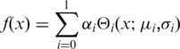
We modeled the distribution of the IgG control data with a truncated normal (truncated at 0.5) distribution, a lognormal distribution or a truncated Poisson distribution (0 was excluded as possible value). For the sample data, we used two-component mixture models of normal or lognormal distributions as given by

(1)

where denotes the probability density functions, α_i represents the fraction which the i-th component contributes to the total and µ_i and σ_i are the parameters of the i-th component. The fits were determined by a Java implementation in EpiChIP of the expectation maximization algorithm (EM) (20). The resulting likelihood values were used to calculate the bayesian information criteria (BICs) (21). In case of the fits to the not-XSET processed IgG control data, we used numerical optimization of the likelihood function with the R function ‘optim’.

Upon setting a threshold for the ChIP-seq value, the FDR of background (BG) genes with regards to histone modified (HM) genes can be defined (FDR_High):

(2)

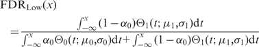
Analogous calculations were carried out for the negative groups (FDR_Low), by swapping the two distributions and integrating from to x:

(3)

The threshold x for a defined FDR was determined so that Values above or below the thresholds determined for FDR_High or FDR_Low, respectively, were classified as HM or BG, respectively.

Implementation in EpiChIP

The analysis methods were implemented in EpiChIP as described above. EpiChIP was written in Java.

MACS analysis

The MACS program (version 1.3.7.1) was downloaded from http://liulab.dfci.harvard.edu/MACS/ and run under standard parameters except for ‘tsize’ which was increased to 36 and ‘m-fold’ which was decreased to 20. Both the H3K9/14ac samples as well as the IgG control were used as input except for the H3K27me3 sample, for which no control was available (8).

RESULTS

Identifying the globally most highly enriched regions of genes

We generated ChIP-seq data for the H3K9/14 histone acetylation in murine Th2 cells, a cell type that is part of the immune system and can be obtained in large numbers ex vivo. Supplementary Figure S1A and S1B demonstrate characterization of the cell type by protein and mRNA expression of cell-type-specific genes (Il13 and Gata3). To test the experimental background of the ChIP-seq method, we also prepared data from a control sample where we used a non-specific IgG antibody during the immunoprecipitation step. Supplementary Table S1 shows that we were able to map ∼10–27 million reads per ChIP-seq reaction of which ∼80% were uniquely mappable.

We processed the mapped read positions based on the ‘XSET’ method (22), by assuming our 36-bp sequence reads to be the ends of fragments of an average size of 200 bp. We then converted this into a distribution of read density along the chromosomes. Supplementary Figure S1C shows the resulting peak landscape along the Gata3 gene.

In order to find the region relative to a specific genomic mark (5′- or 3′-end of genes, exons or introns) where histone modifications are present, we first aligned all the genomic objects (genes, exons or introns) according to either 5′- or 3′-ends and depicted an overall landscape of read distribution along the genomic objects –x-axis being the base pair distance relative to the alignment point and y-axis being the number of read-nucleotides per gene at that base pair. Additionally, we stretched or compressed each genomic object to the same length and obtained another set of landscapes in terms of ‘percentage length’. Within these landscapes, global peaks are detected as region with a read enrichment of >40% of the largest value and no <150 bp in width (2% in the case of percentage length). This is used as a window for further analysis (for a further discussion of the window detection procedure, please see the discussion in the Supplementary Data). Once the windows are identified across all genomic annotations, their importance is determined and ranked by how many reads fall into each window normalized to the window width.

In the case of our H3K9/14ac data set, the most enriched window is from 400-bp upstream of the transcription start site (TSS) to 807-bp downstream. In contrast, the IgG control distribution is much flatter, showing only a slight enrichment at TSSs (Figure 1A). Therefore, we used this window for further analysis. It is also interesting to note that intron/exons junctions featured small peaks.

Figure 1.

ChIP-seq data distribution for the H3K9/14ac histone modification. (A) The cumulative read density for the whole genome is shown from −5 kb to +5 kb relative to TSSs. The H3K9/14ac sample (blue) shows a strong enrichment within the first kb downstream from TSS. The IgG control (black) shows a much weaker enrichment in this region. (B) Kernel density estimates of the distributions of all genes with respect to NLCS values within the window from −400 to +807 bp with respect to TSSs. IgG control (black/top) and H3K9/14ac sample (blue/bottom) are shown on linear (left) and log₂ (right) scales. The dotted lines represent the signal distributions of random intergenic regions of the same window size. The shapes of the data distributions suggest that the H3K9/14ac sample consists of two separate distributions, the experimental/biological background (BG) and the actual histone-modification signal (HM). (C) Mathematical modeling of the IgG control-data distribution. The genome-wide distribution of the numbers of sequencing reads within the −400/+807 bp window from TSSs (not XSET processed) are shown as a histogram on linear (left) and log₂ (right) scales. Numerical maximum likelihood fits of truncated Poisson (red), normal (cyan), lognormal (purple) and truncated normal distributions (green) are overlaid. Parameters and BICs are given in Supplementary Table S2.

Clearly, this strategy can be applied to any type of chromosomal annotation, including, for example, enhancer annotations. Furthermore, it can be applied to ChIP-seq data for proteins other than histones, e.g. TFs, RNA polymerase and so forth, to search for globally enriched regions relative to gene or enhancer annotations for instance.

Gene-by-gene quantification of histone modification levels: signal versus noise

Based on the optimal window of H3K9/14ac around TSSs, we extracted the peak area within the window for each gene individually. We normalize this value by the total area and define it as the normalized locus-specific chromatin state (NLCS). When we display the global distribution of this value for all genes as a density plot, the number of genes decays rapidly as the value increases for both the control and the H3K9/14ac sample. The H3K9/14ac sample features an extra shoulder (Figure 1B), which is emphasized by log-transforming the data, and suggests that the sample data is a sum of two separate but overlapping distributions (Figure 1B). This is reminiscent of flow cytometry data, where protein staining with fluorescent antibodies often leads to two separate distributions of log-transformed fluorescence intensity per cell, one corresponding to auto-fluorescence or background staining, the other to the subpopulation of cells expressing the protein (23).

The major question is what the natures of the two subpopulations of our sample are. From the log transformation, we observe that the NLCS of the IgG control displays only one peak (apart from the smaller spikes which are due to log transformation) with NLCS values very similar to the left peak of the H3K9/14ac data. This observation indicates that the left peak is likely due to the background noise. This is also confirmed by a study of the genomic background within the samples. Here, we randomly selected fragments with the optimal window width from the intergenic regions and plotted the distribution of the NLCS values (Figure 1B, dotted lines). For the IgG control, the resulting distribution largely overlaps with the distribution based on the window (Figure 1B). The small shift to the left probably reflects the slight TSS enrichment we have seen previously (Figure 1A). The H3K9/14ac intergenic distribution also lies slightly toward the left of the left peak, and its large overlap with the left peak suggests that the left peak consists of a large proportion of experimental noise and possibly biological noise, which should be filtered from the right peak—the genes with true modification signals. Therefore, we designate these two to-be-separated subpopulations of genes as BG (background) and HM (histone modification) (Figure 1B).

In order to separate HM from BG, the shape of each distribution has to be elucidated. Although most studies assume that the experimental background of high-throughput sequencing follows Poisson distributions (22), some studies suggest that the ChIP-seq background is not simple (24,25). In order to directly compare a Poisson fit to possible alternatives (normal, log normal or truncated normal), we extracted from our IgG control data the number of complete sequencing reads that map to the TSS window. We excluded genes with zero values (2% in H3K9/14ac and 18% in IgG, which are reasonably low portions) because a discontinuity of the distribution is present at zero due to the lack of resolution and hence not suitable for modeling. We calculated the Bayesian Information Criterion (BIC) (21) as an indication of the goodness-of-fit. The fitting results suggest that the two-parameter distributions (normal, lognormal and truncated normal) fit much better than the one-parameter Poisson model. Amongst the two-parameter distributions, the truncated (at 0.5) normal distribution fits best to the IgG control distribution (Figure 1C, see Supplementary Table S2 for parameters).

The shape of the HM distribution of our H3K9/14ac sample suggests that a normal or lognormal function would fit the distribution of this group of genes well too. In order to determine contributions of the BG and HM groups to the total distribution of the data, we fit two-component mixture models of various combinations of normal and lognormal distributions (two normal, two lognormal, mixed lognormal and normal) to the NLCS distributions by using the expectation EM (20). Due to the complexity of parameter estimation, the truncated normal distribution was not included here.

All of the tested models fit the data well, with very close BICs (normal+lognormal, Figure 2A, for other combinations, see Supplementary Figure S2 and Table S3). For further analysis, we picked the model that represents BG and HM groups as normal and lognormal (Figure 2A), respectively, as they best reproduce the shape of the actual distribution.

Figure 2.

(A) Mathematical modeling of the H3K9/14ac sample data. (A) combination of a normal (for BG) and a lognormal distribution (for HM) was fit to the NLCS data (from the −400/+807-bp TSS window, as shown in Figure 1B). The experimental data is shown in blue, the BG curve in orange, the HM curve in purple, the sum of the two latter in red. The fit was based on parameter estimation by expectation maximization. Parameters are given in Supplementary Table S3. Alternative fits are shown in Supplementary Figure S2. The grey lines indicate the thresholds at FDR = 0.01. (B) Expression levels of genes in the BG and HM categories. The expression levels are significantly different (P < 2.2 × 10⁻¹⁶, one-sided Wilcoxon test). (C) Plot of histone modification versus gene expression for each gene. The heatmap represents a 2D-kernel density estimate of ∼15 000 genes.

Distinguishing histone-modified genes from background

Based on the parameterization of the BG and HM distributions, we can now quantify the overlap between the two groups of genes at any point of the data distribution. An FDR can be set which gives a minimum threshold of NLCS above which the probability of finding a BG gene is below the desired FDR value. Genes with NLCS values higher than the minimum threshold can then be classified within the desired FDR. Similarly, BG genes can be obtained by a maximum threshold, which means that for genes below this threshold, the probability to find HM genes is less than the FDR.

We chose an FDR of 0.01 and performed a binary classification of genes for both the BG and HM groups of genes (Figure 2A). Of the total 21 326 genes, 20 424 could be classified, with the remainder of 902 genes in the intermediate region where the BG and HM distributions overlap extensively. Our classification agrees with the current understanding of T helper cell biology as genes expressed exclusively in Th2 cells such as Gata3, Il4 and Il13 are found in the HM group. Genes such as Ifng and Il17a, on the other hand, which are known to be expressed in Th1 and Th17 cells (and not in Th2 cells), respectively, are found in the BG category.

Integration with expression data

In order to probe the biological meaning of the two sets of genes, we extracted the expression levels of genes in each category from published microarray data for the same cell type (19). Genes in the HM category were expressed at significantly higher levels (P < 2.2 × 10⁻¹⁶, one-sided Wilcoxon rank-sum test) than those classified as BG (Figure 2B).

To further study the relationship between histone modification and expression, we display the combined histone modification and expression data for all genes as a 2D density plot, with the color denoting the density of genes at particular spots. This representation of the NLCS versus gene expression data supports the concept of BG/HM separation, as two clearly identifiable groups of genes are visible, which correspond to either high expression and presence of H3K9/14ac histone modification or low/off expression and histone modification at background levels, respectively (Figure 2C). Comparison with Figure 2B shows that the expression levels of the BG/HM classified genes agree very well with the expression levels of the two groups of genes in Figure 2C.

These results demonstrate that the global pattern of ChIP-seq signal for a histone modification allows us to distinguish experimental or biological background from the actual signal, if the data is extracted from each gene individually based on a sequence window. This in turn makes it possible to classify genes into background and histone-modified genes and yields estimates for the genome-wide fraction of modified genes. The close agreement with the expression data demonstrates the validity and power of our approach. An overview of our analysis strategy is given in Figure 3.

Figure 3.

Overview of the analysis strategy.

EpiChIP software

Based on our observations, we have developed the ‘EpiChIP’ software, which allows the analysis of ChIP-seq experiments in a similar way to the approach described above. EpiChIP is a platform independent desktop application and comes with a user-friendly graphical interface that does not require any programming skills. The user supplies EpiChIP with files of sequencing reads that were mapped by any of three common mapping programs (Maq, Eland, Bowtie) or BED files. Then, based on a gene annotation file (RefSeq for mouse and human are included with EpiChIP) or user-defined custom annotations, one or more sequence windows with respect to genomic coordinates can be chosen. These may include regions around the TSS or end of a gene, the sequences at intron/exon boundaries, etc. EpiChIP then determines the density of paired-end or XSET-processed single-end reads along the sequence window(s) for each gene.

The genome-wide distribution of the data along the window(s) is displayed, peak detection is performed and further window-specific information such as the percentage of total peak area that falls into the various windows is output. This enables the user to decide which window should be used for the further analysis.

EpiChIP allows the user to upload a control sample and overlay it with the plots generated for the actual sample as a further means to test the presence of specific signal in the sample (in addition to the presence of bimodality in the global data distribution).

Based on the selected window, the NLCS value for each individual gene is then extracted and the distribution of NLCS among all genes is displayed on linear or log₂ scale. Currently, our program fits combinations of normal or lognormal distributions to this data and displays all relevant fitting parameters. An upgrade allowing for further distributions is planned. EpiChIP lets the user decide on an FDR and saves the resulting gene lists in files that can be used for further analysis.

In the case that the 1D distribution does not allow one to clearly identify two peaks, we also included a feature for linking the data to a second data set, such as gene expression data, and displaying it as a heatmap as in Figure 2C. The user can then encircle groups of genes and save them to files.

EpiChIP is downloadable for multiple platforms from http://epichip.sourceforge.net/index.html. The web site will be regularly updated and contains a tutorial, a detailed documentation, an FAQ list and the mapped Th2 sample and control files which can be used as demos for exploring EpiChIP functions.

Examples

We have tested EpiChIP on published ChIP-seq datasets for 36 histone modifications, RNA PolII and CTCF binding and H2AZ histones in human Th cells (8,26). EpiChIP confirmed previously described genomic distributions of the studied modifications and identified optimal windows varying from <200 bp to >5 kb in length in 14 out of 16 histone acetylations and 14 out of 20 methylations (Supplementary Table S4). The smaller number of optimal windows that were identified among the methylations probably reflects the more diverse pattern of histone methylations, which, in contrast to the acetylations, can also be associated with repressed transcription and generally show more intricate distributions, such as the marking of expressed exons (11,27).

In all cases where an optimal window was detected, the bimodality in the log NLCS-value distribution was observed. We show screenshots of the curve fittings EpiChIP performed on five different examples. For H3K9me1, we used the window EpiChIP detected automatically, from −987 to +2568 bp with respect to TSSs (Figure 4A). For H3K27me3, where a peak at TSSs is not strong but present, we manually picked a window from the TSS to 2-kb downstream (Figure 4B). Finally, we picked a window from the start of exons to +300-bp downstream (the first exons and introns of all genes are excluded by EpiChIP to avoid signal overlaps from TSSs) for the H3K36me3 modification (Figure 4C). In addition, we show curve fittings to two canonical activating histone modifications, H3K9ac (Supplementary Figure S3A) and H3K4me3 (Supplementary Figure S3B). The EpiChIP curve fitting yielded good fits in all cases and allowed successful separation of HM from BG. This illustrates the functionality of our program and demonstrates the wide applicability to different types of histone modifications and other data.

Figure 4.

EpiChIP screenshots for analysis examples. Types of histone modifications and analysis windows as indicated (A) H3K9me1, (B) H3K27me3 and (C) H3K36me3.

We further studied the consistency of EpiChIP with one of the most widely used peak-finding program, MACS (28). We used the list of peaks MACS identified in our H3K9/14ac sample to represent a new starting dataset for EpiChIP and compared its output on the MACS peaks with the EpiChIP output on the original data. We found that the optimal window for the MACS peaks (from −402 to +841 bp at TSSs, Supplementary Figure S4A) was very similar to the one identified in the original data (see above). Moreover, once we used this window to calculate the NLCS values and perform a classification into BG and HM, the overlap between HM genes and genes that had a MACS peak in the same window was very high (Supplementary Figure S4B). This good agreement supports our concept of background modeling based on the genome-wide data distribution. Furthermore, it demonstrates that EpiChIP and peak-finding programs can be used in a complementary manner. As a further example, we compared the performance of EpiChIP and MACS on the H3K27me3 dataset as described above. When we select for all genes that have MACS peaks within the region from 0 to 2 kb with respect to TSS and plot the expression levels of those, we find that many of the MACS-selected genes are still expressed at high levels, whereas the proportion of EpiChIP-‘HM’ genes that are expressed are lower and within the range expected from the FDR (Supplementary Figure S5).

DISCUSSION

We demonstrate here a novel way for analyzing ChIP-seq data for histone modifications. The strengths of our approach are the focus on fixed sequence windows with respect to genomic coordinates, the extraction of data on a single-gene basis, the analysis of the genome-wide distribution of the data and the modeling of the background by curve fitting. As our findings show, this reveals a number of undiscovered features of the structure of the data, which is invaluable to understanding the underlying biological mechanisms.

Most other programs for analyzing ChIP-seq data are aimed at the detection of peaks, which is usually not restricted to specific regions along the genome. This approach is useful for TFs and enhancer-marking histone modifications such as the H3K4me1 mark (29). However, it is not fully suited to most other histone modifications, which are not found as sharp peaks but usually cover larger regions associated with gene coordinates. By considering a defined, fixed sequence window with respect to gene positions, there is no need for EpiChIP to separately estimate the background within a shifting window at each point to account for heterogeneous regions along the genome. Instead, our global approach clearly allows the distinction between signal and background. Thus, EpiChIP makes minimal assumptions and does not attempt ‘blind folded’ background estimation.

Detection and/or shape of the background distribution will depend on parameters such as the total number of sequencing reads, the frequency of the studied histone modification, the biological noise associated with it and the experimental noise of the used method. The higher the read number, the fewer genes will have zero reads, and the background distribution will become better defined. Improvements of the current ChIP-seq techniques will likely lead to reductions of the experimental background noise. This might be balanced by increased sensitivity, possibly revealing distributions of biological background noise with more accuracy.

The EpiChIP analysis strategy does not make direct use of the control sample in the background/signal discrimination process. Although this has certain drawbacks such as the loss of position-specific background information, this is largely compensated for by the window approach. For instance, our IgG control shows slight enrichment close to TSSs which is, however, similar at all TSSs throughout the genome and not due to a few outliers. For analysis of the actual sample, the window approach is therefore expected to yield similar levels of background at all analyzed spots. A major advantage of determining the background internally is that the actual distribution itself is used, allowing a more accurate determination of the real background. Since there is a trade-off of sequencing read numbers between signal and background in the experiment but not in the control, the background levels in the actual sample might be lower in terms of NLCS than in the control. The internal curve fitting for signal/background discrimination is not affected by this. In any case, inclusion of controls in ChIP-seq experiments provides useful information about the characteristics of the background distribution.

The successful analysis of several different types of histone modifications with EpiChIP indicates that our approach is generally applicable to ChIP-seq data for histone modifications. Our binary classification provides an easy way to compare and/or integrate large datasets of many epigenetic marks in terms of absence/presence of marks at genes. Thus analysis tools such as clustering, principal component analysis, etc. can readily be run across all genes in a genome. Integration with expression data also becomes very easy and might reveal associations of modules of epigenetic modifications with certain gene expression levels.

EpiChIP can also be used with custom genomic annotations. Thus it can serve as a tool for directly analyzing the dependence between a ChIP-seq data set and a set of chromosomal annotations derived from other ChIP-seq data sets, RNA-seq data sets or yet another source. In this way, EpiChIP provides new perspectives for discovering novel patterns and formulating hypotheses with regards to transcriptional regulation.

SUPPLEMENTARY DATA

Supplementary Data are available at NAR Online.

FUNDING

Funding for open access charge: Medical Research Council.

Conflict of interest statement. None declared.

REFERENCES

- 1.Solomon MJ, Larsen PL, Varshavsky A. Mapping protein-DNA interactions in vivo with formaldehyde: evidence that histone H4 is retained on a highly transcribed gene. Cell. 1988;53:937–947. doi: 10.1016/s0092-8674(88)90469-2. [DOI] [PubMed] [Google Scholar]
- 2.Ren B, Robert F, Wyrick JJ, Aparicio O, Jennings EG, Simon I, Zeitlinger J, Schreiber J, Hannett N, Kanin E, et al. Genome-wide location and function of DNA binding proteins. Science. 2000;290:2306–2309. doi: 10.1126/science.290.5500.2306. [DOI] [PubMed] [Google Scholar]
- 3.Shendure J, Ji H. Next-generation DNA sequencing. Nat. Biotechnol. 2008;26:1135–1145. doi: 10.1038/nbt1486. [DOI] [PubMed] [Google Scholar]
- 4.Park PJ. ChIP-seq: advantages and challenges of a maturing technology. Nat. Rev. Genet. 2009;10:669–680. doi: 10.1038/nrg2641. [DOI] [PMC free article] [PubMed] [Google Scholar]
- 5.Robertson G, Hirst M, Bainbridge M, Bilenky M, Zhao Y, Zeng T, Euskirchen G, Bernier B, Varhol R, Delaney A, et al. Genome-wide profiles of STAT1 DNA association using chromatin immunoprecipitation and massively parallel sequencing. Nat. Methods. 2007;4:651–657. doi: 10.1038/nmeth1068. [DOI] [PubMed] [Google Scholar]
- 6.Johnson DS, Mortazavi A, Myers RM, Wold B. Genome-wide mapping of in vivo protein-DNA interactions. Science. 2007;316:1497–1502. doi: 10.1126/science.1141319. [DOI] [PubMed] [Google Scholar]
- 7.Farnham PJ. Insights from genomic profiling of transcription factors. Nat. Rev. Genet. 2009;10:605–616. doi: 10.1038/nrg2636. [DOI] [PMC free article] [PubMed] [Google Scholar]
- 8.Barski A, Cuddapah S, Cui K, Roh TY, Schones DE, Wang Z, Wei G, Chepelev I, Zhao K. High-resolution profiling of histone methylations in the human genome. Cell. 2007;129:823–837. doi: 10.1016/j.cell.2007.05.009. [DOI] [PubMed] [Google Scholar]
- 9.Heintzman ND, Stuart RK, Hon G, Fu Y, Ching CW, Hawkins RD, Barrera LO, Van Calcar S, Qu C, Ching KA, et al. Distinct and predictive chromatin signatures of transcriptional promoters and enhancers in the human genome. Nat. Genet. 2007;39:311–318. doi: 10.1038/ng1966. [DOI] [PubMed] [Google Scholar]
- 10.Roh TY, Cuddapah S, Cui K, Zhao K. The genomic landscape of histone modifications in human T cells. Proc. Natl Acad. Sci. USA. 2006;103:15782–15787. doi: 10.1073/pnas.0607617103. [DOI] [PMC free article] [PubMed] [Google Scholar]
- 11.Kolasinska-Zwierz P, Down T, Latorre I, Liu T, Liu XS, Ahringer J. Differential chromatin marking of introns and expressed exons by H3K36me3. Nat. Genet. 2009;41:376–381. doi: 10.1038/ng.322. [DOI] [PMC free article] [PubMed] [Google Scholar]
- 12.Andersson R, Enroth S, Rada-Iglesias A, Wadelius C, Komorowski J. Nucleosomes are well positioned in exons and carry characteristic histone modifications. Genome Res. 2009;19:1732–1741. doi: 10.1101/gr.092353.109. [DOI] [PMC free article] [PubMed] [Google Scholar]
- 13.Schwartz S, Meshorer E, Ast G. Chromatin organization marks exon-intron structure. Nat. Struct. Mol. Biol. 2009;16:990–995. doi: 10.1038/nsmb.1659. [DOI] [PubMed] [Google Scholar]
- 14.Shin H, Liu T, Manrai AK, Liu XS. CEAS: cis-regulatory element annotation system. Bioinformatics. 2009;25:2605–2606. doi: 10.1093/bioinformatics/btp479. [DOI] [PubMed] [Google Scholar]
- 15.Statham AL, Strbenac D, Coolen MW, Stirzaker C, Clark SJ, Robinson MD. Repitools: an R package for the analysis of enrichment-based epigenomic data. Bioinformatics. 2010;26:1662–1663. doi: 10.1093/bioinformatics/btq247. [DOI] [PMC free article] [PubMed] [Google Scholar]
- 16.Hebenstreit D, Giaisi M, Treiber MK, Zhang XB, Mi HF, Horejs-Hoeck J, Andersen KG, Krammer PH, Duschl A, Li-Weber M. LEF-1 negatively controls interleukin-4 expression through a proximal promoter regulatory element. J. Biol. Chem. 2008;283:22490–22497. doi: 10.1074/jbc.M804096200. [DOI] [PMC free article] [PubMed] [Google Scholar]
- 17.Wilson NK, Miranda-Saavedra D, Kinston S, Bonadies N, Foster SD, Calero-Nieto F, Dawson MA, Donaldson IJ, Dumon S, Frampton J, et al. The transcriptional programme controlled by the stem cell leukaemia gene Scl/Tal1 during early embryonic haematopoietic development. Blood. 2009;113:5456–5465. doi: 10.1182/blood-2009-01-200048. [DOI] [PubMed] [Google Scholar]
- 18.Langmead B, Trapnell C, Pop M, Salzberg SL. Ultrafast and memory-efficient alignment of short DNA sequences to the human genome. Genome Biol. 2009;10:R25. doi: 10.1186/gb-2009-10-3-r25. [DOI] [PMC free article] [PubMed] [Google Scholar]
- 19.Wei L, Vahedi G, Sun HW, Watford WT, Takatori H, Ramos HL, Takahashi H, Liang J, Gutierrez-Cruz G, Zang C, et al. Discrete roles of STAT4 and STAT6 transcription factors in tuning epigenetic modifications and transcription during T helper cell differentiation. Immunity. 2010;32:840–851. doi: 10.1016/j.immuni.2010.06.003. [DOI] [PMC free article] [PubMed] [Google Scholar]
- 20.Dempster AP, Laird NM, Rubin DB. Maximum Likelihood from Incomplete Data Via Em Algorithm. J. Roy Stat. Soc. B Met. 1977;39:1–38. [Google Scholar]
- 21.Schwarz G. Estimating Dimension of a Model. Ann. Stat. 1978;6:461–464. [Google Scholar]
- 22.Pepke S, Wold B, Mortazavi A. Computation for ChIP-seq and RNA-seq studies. Nat. Methods. 2009;6:S22–S32. doi: 10.1038/nmeth.1371. [DOI] [PMC free article] [PubMed] [Google Scholar]
- 23.Shapiro HM. Practical Flow Cytometry. 3rd edn. New Jersey: Wiley-Liss, Hoboken; 2003. [Google Scholar]
- 24.Bentley DR, Balasubramanian S, Swerdlow HP, Smith GP, Milton J, Brown CG, Hall KP, Evers DJ, Barnes CL, Bignell HR, et al. Accurate whole human genome sequencing using reversible terminator chemistry. Nature. 2008;456:53–59. doi: 10.1038/nature07517. [DOI] [PMC free article] [PubMed] [Google Scholar]
- 25.Rozowsky J, Euskirchen G, Auerbach RK, Zhang ZD, Gibson T, Bjornson R, Carriero N, Snyder M, Gerstein MB. PeakSeq enables systematic scoring of ChIP-seq experiments relative to controls. Nat. Biotechnol. 2009;27:66–75. doi: 10.1038/nbt.1518. [DOI] [PMC free article] [PubMed] [Google Scholar]
- 26.Wang Z, Zang C, Rosenfeld JA, Schones DE, Barski A, Cuddapah S, Cui K, Roh TY, Peng W, Zhang MQ, et al. Combinatorial patterns of histone acetylations and methylations in the human genome. Nat. Genet. 2008;40:897–903. doi: 10.1038/ng.154. [DOI] [PMC free article] [PubMed] [Google Scholar]
- 27.Wang Z, Schones DE, Zhao K. Characterization of human epigenomes. Curr. Opin. Genet. Dev. 2009;19:127–134. doi: 10.1016/j.gde.2009.02.001. [DOI] [PMC free article] [PubMed] [Google Scholar]
- 28.Zhang Y, Liu T, Meyer CA, Eeckhoute J, Johnson DS, Bernstein BE, Nussbaum C, Myers RM, Brown M, Li W, et al. Model-based analysis of ChIP-Seq (MACS) Genome Biol. 2008;9:R137. doi: 10.1186/gb-2008-9-9-r137. [DOI] [PMC free article] [PubMed] [Google Scholar]
- 29.Heintzman ND, Hon GC, Hawkins RD, Kheradpour P, Stark A, Harp LF, Ye Z, Lee LK, Stuart RK, Ching CW, et al. Histone modifications at human enhancers reflect global cell-type-specific gene expression. Nature. 2009;459:108–112. doi: 10.1038/nature07829. [DOI] [PMC free article] [PubMed] [Google Scholar]
Associated Data
This section collects any data citations, data availability statements, or supplementary materials included in this article.