Network component analysis: Reconstruction of regulatory signals in biological systems

Abstract

High-dimensional data sets generated by high-throughput technologies, such as DNA microarray, are often the outputs of complex networked systems driven by hidden regulatory signals. Traditional statistical methods for computing low-dimensional or hidden representations of these data sets, such as principal component analysis and independent component analysis, ignore the underlying network structures and provide decompositions based purely on a priori statistical constraints on the computed component signals. The resulting decomposition thus provides a phenomenological model for the observed data and does not necessarily contain physically or biologically meaningful signals. Here, we develop a method, called network component analysis, for uncovering hidden regulatory signals from outputs of networked systems, when only a partial knowledge of the underlying network topology is available. The a priori network structure information is first tested for compliance with a set of identifiability criteria. For networks that satisfy the criteria, the signals from the regulatory nodes and their strengths of influence on each output node can be faithfully reconstructed. This method is first validated experimentally by using the absorbance spectra of a network of various hemoglobin species. The method is then applied to microarray data generated from yeast Saccharamyces cerevisiae and the activities of various transcription factors during cell cycle are reconstructed by using recently discovered connectivity information for the underlying transcriptional regulatory networks.

High-throughput techniques in biology, such as DNA microarray (1), have generated a large amount of data that can potentially provide systems-level information regarding the underlying dynamics and mechanisms. These high-dimensional output data are typically the end products of low-dimensional regulatory signals driven through an interacting network. As illustrated in Fig. 1, the relationship between the lower dimensional regulatory signals (or states) and output data can be modeled by a bipartite networked system, where the output signals (e.g., gene expression levels) are generated by weighted functions of the intracellular states (e.g., the activity of the transcription factors). A major challenge in systems biology is to derive methodologies for simultaneous reconstructions of the hidden dynamics of the regulatory signals.

Fig. 1.

A regulatory system in which the output data are driven by regulatory signals through a bipartite network. Network component analysis (NCA) takes advantage of partial network connectivity knowledge and is able to reconstruct regulatory signals and the weighted connectivity strength. For example, if a regulatory node or factor is known from experimental evidence to have negligible or no effect on an output signal, then the corresponding edge may be removed or, equivalently, its weight may be set to zero. As discussed in the text, such qualitative knowledge for a number of large biological systems is becoming available through high-throughput experiments. In contrast, traditional methods such as PCA and ICA depend on statistical assumptions and cannot reconstruct regulatory signals or connectivity strength.

In recent years, statistical techniques for determining low-dimensional representations of high-dimensional data sets, e.g., principal component analysis (PCA) (2) or singular value decomposition (3–5) and independent component analysis (ICA) (6), have been applied successfully to deduce biologically significant information from high-throughput data sets. It is important to recognize that such dimensionality reduction techniques are not designed to address the hidden dynamics reconstruction problem addressed in this article. For example, PCA and ICA both would generate linear networks for interpreting the observed data set, where the regulatory signals are constrained to be mutually orthogonal and statistically independent, respectively. However, both the reconstructed signals and the networks do not match the real system and provide only a phenomenological modeling of the observed data. In fact, as we show later, it is impossible to reconstruct the underlying regulatory state without additional constraints.

Fortunately, for many biological systems partial prior knowledge about the connectivity patterns of the bipartite networks is beginning to become available via high-throughput experiments (7) or data mining of interaction knowledge (8–10), even though the detailed mechanisms remain undiscovered. Currently, however, it is unclear whether and how such qualitative connectivity information can be used to generate quantitative regulatory signals and further network details. Motivated by this pressing question in systems biology, we first derive a set of criteria for such prior connectivity information to be sufficient to solve the reverse engineering problem. We then provide a framework for the reconstruction process once such criteria are satisfied. This approach, termed NCA, is experimentally validated by using absorbance spectra of reconstructed biological solutions where the mixing (connectivity) pattern is known. Finally, we demonstrate the utility of NCA to genomewide gene expression data in yeast Saccharomyces cerevisiae during cell cycle. As the bipartite network shown in Fig. 1 can represent many different types of data that are determined by multiple competing factors, the method developed here, NCA, can be applied to a large number of problems, where qualitative network structural information is available.

Mathematical Framework

The multidimensional data are organized in a format where M samples (or time points) of N output variables (such as the expression ratio of transcripts) is collected in the rows of a matrix [E] (size: N rows × M columns). We seek to reconstruct a model of the type:

[1]

Here the matrix [P] (size: L × M) consists of samples of L regulatory signals, where L is in general much smaller than N, thus resulting in the reduction in dimensionality. The matrix [A] (size: N × L) encodes the connectivity strength between the regulatory layer and the output signals (Fig. 1). Eq. 1 represents the linear approximation of any detailed mechanistic model and is commonly used as the first approximation when the latter is unavailable.

The decomposition of a matrix [E] into two matrices, [A] and [P], according to Eq. 1 is an inverse problem whose solution is in general not uniquely defined unless further assumptions on the matrices [A]or[P] are made. This can be seen by introducing a nonsingular matrix [X] (L × L) such that [Ā] = [A][X] and [P̄] = [X^–1][P], and

[2]

Thus, without further constraints, [E] cannot be uniquely decomposed to [A] and [P] according to Eq. 1. Conventional approaches, such as PCA and ICA, typically seek a matrix [A] such that the resulting reconstructed signal matrix [P] satisfies orthogonality or independence criteria, respectively. When dealing with data generated from structured networks, such as biological systems, these decomposition techniques present two drawbacks. First, the implicit statistical assumptions on the regulatory signals lack biological foundation. Second, the reconstructed connectivity structure is unlikely to be consistent with the underlying network structure. Therefore, we seek a decomposition method that makes no assumption on the statistical properties of the regulatory signals and that, at the same time, allows proper handling of the prior knowledge on the structure characterizing a given system.

Criteria for NCA

According to Eq. 2, multiple [A]s and [P]s can reconstruct data [E] equally well. However, when certain connectivity constraints are imposed on [A], the [X] matrix in Eq. 2 can only be diagonal (for proof, see Appendix 1, which is published as supporting information on the PNAS web site). Furthermore, when [A] has full column rank and [P] has full row rank, Eq. 2 represents all of the possible alternative solutions of the decomposition of [E] (see Appendix 1 for proof). Under these conditions, Eq. 1 results in a unique decomposition of the data, up to a scaling factor. Therefore, certain network structures enable the decomposition of data. This type of decomposition is defined as NCA. In summary, the criteria for NCA to be feasible are:

1. The connectivity matrix [A] must have full-column rank.

2. When a node in the regulatory layer is removed along with all of the output nodes connected to it, the resulting network must be characterized by a connectivity matrix that still has full-column rank. This condition implies that each column of [A] must have at least L-1 zeros.

3. [P] must have full row rank. In other words, each regulatory signal cannot be expressed as a linear combination of the other regulatory signals.

If these criteria are satisfied, the data matrix [E] can be uniquely decomposed to a connectivity matrix [A] and signal matrix [P] when a scaling rule applies. The matrix [A] contains the estimated connectivity strength on each edge, whereas the matrix [P] contains the regulatory signals of each regulatory node.

To test the feasibility of NCA, one first constructs an initial [A] matrix based on knowledge of connectivity. The [A] entry at ith row and jth column (a_ij) represents the control strength of each regulatory node j on output node i. If this pair is not connected, the value for a_ij is zero. Otherwise, it is arbitrarily set to a nonzero number as an initial value. Thus, the [A] matrix has a dimension of N × L, where N is the number of output nodes and L is the number of regulatory nodes (e.g., transcription factors) considered. Given the initial connectivity matrix [A] (N × L), we first test whether it has full column rank (criterion i). If this criterion is satisfied, we then form a set of reduced matrices [Ar_j], by removing the jth column and all of the rows of A corresponding to the nonzero entries of its jth column. For example, if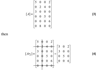 Criterion ii is satisfied, if and only if, for any possible choice of a single regulatory node, the corresponding reduced matrix has rank equal to L-1.

Criterion iii cannot be tested a priori, but it implies the necessary condition that L (the number of regulatory nodes) must be less than M (the number of data points). If L is indeed less than M, the matrix [P] is likely to have full row rank for real biological data. This rank condition should be checked after [P] is obtained from NCA. If L > M, a subnetwork should be generated to reduce L. This can be done by removing selected regulatory nodes together with all of the output nodes they control. If the subsystem satisfy L < M, then proceed to test the other criteria. If the subsystem satisfies all three criteria, then it is NCA compliant.

A simple example is shown in Fig. 2, which presents a completely identifiable network (Fig. 2a) and an unidentifiable network (Fig. 2b), although the two matrices have an identical number of constraints (zero entries). The network in Fig. 2b does not satisfy the identifiability criterion because of the connectivity pattern of R₃.

Fig. 2.

A completely identifiable network (a) and an unidentifiable network (b). Although the two initial [A] matrices describing the network matrices have an identical number of constraints (zero entries), the network in b does not satisfy the identifiability conditions because of the connectivity pattern of R₃. The edges in red are the differences between the two networks.

Method for NCA

Once the identifiability of a given system has been established, the regulatory signals, [P], and the connectivity strength, [A], can be reconstructed through the following procedure. An initial guess for the connectivity matrix A is formed by setting to zero all of the elements corresponding to missing edges between the regulatory layer and the output layer. The remaining elements can be initialized to an arbitrary value. Because the experimental measurements are noisy, an exact solution to the decomposition problem does not exist in general. However, when the above NCA criteria are satisfied, the estimation problem becomes well posed, and a solution that provides the best fit in the least-squares sense can be computed. We proceed by minimizing the following objective function:

[5]

where Z₀ is the topology induced by the network connectivity pattern. Additional constraints on the nature of the regulation (positive or negative) can also be included in the optimization framework, but are not strictly required by the method in general.

The above objective function is equivalent to a constrained maximum-likelihood procedure in the presence of Gaussian noise with independent and identically distributed components. The actual estimation of [A] and [P] is performed by using a two-step least-squares algorithm, which exploits the biconvexity properties of linear decompositions (Appendix 2, which is published as supporting information on the PNAS web site). The variability of our estimates is assessed by using a bootstrap procedure (Appendix 3, which is published as supporting information on the PNAS web site).

Normalization of [A] and [P] can be achieved by a nonsingular diagonal matrix [X] in Eq. 2. The elements of [X] should be selected according to the physical or biological nature of the data set. As an example, the columns of [A] (for each regulatory node across all of the output node) can be normalized so that the mean absolute value of the nonzero elements is equal to the number of controlled output nodes. With this normalization, the rows of [P] for different regulatory nodes represent the average effect of the regulator on the output nodes it controls, and the columns of [A] represent the relative control strength for the same regulator on different output nodes.

Experimental Validation of NCA

To verify experimentally the NCA method described above, we used a network of seven hemoglobin solutions as a test case. Each solution contains a combination of three components: oxyhemoglobin, methemoglobin, and cyano-methemoglobin. These solutions were prepared according to Appendix 4, which is published as supporting information on the PNAS web site, and the absorbance spectra were taken between 380 and 700 nm with 1-nm increments. According to Beer–Lambert law, the absorbance spectra can be described as follows:

[6]

where the rows of [Abs] are the absorbance spectra of each solution at each wavelength, the columns of the connectivity matrix [C] are the concentrations of each component, and the rows of [ε] are the spectra of pure components. The connectivity diagram of this solution network is shown in Fig. 3a, where the components of the four solutions are known, but the concentration of each component and the pure-component spectra are assumed to be unknown and will be determined from the solution spectra by using NCA.

Fig. 3.

Experimental validation of the NCA method using absorbance spectra of hemoglobin solutions. OxyHb, oxyhemoglobin; MetHb, methemoglobin; CyanoHb, cyano-methemoglobin. (a) The connectivity (mixing) diagram of the seven Hb solutions from three pure components that serve as the regulatory nodes. (b) The regulatory signals (pure component spectra) derived from NCA agree well with the true values, whereas those derived from PCA or ICA do not.

The connectivity matrix [C] is initiated by using nonzero random numbers and 0s for components present or absent, respectively, in the solution according to Fig. 3a. The initial [C] matrix was verified to satisfy the NCA criteria. The decomposition was carried out according to the NCA algorithm briefly described above and detailed in Appendix 2. Results (Fig. 3b) show that the pure component spectra ([ε]) resulted from NCA agree well with the true spectra obtained from independent measurements of pure components. Despite the similarity among the pure component spectra, NCA was able to resolve the differences. In contrast, singular value decomposition or ICA cannot reconstruct the pure component spectra faithfully (Fig. 3b). In addition, the concentrations estimated from the [C] matrix show satisfactory agreement with the true concentrations (Table 1). Note that the spectra were decomposed by using only the known components, but not the concentrations of the solutions. However, the NCA method was able to simultaneously determine the concentrations of each component and the spectra of pure components.

Table 1. Concentrations of the hemoglobin solutions estimated from the NCA analysis agree reasonably well with the true values (in parentheses).

Mixture	OxyHb, μM	MetHb, μM	CyanoHb, μM
M1	0.13 (0.13)	3.8 (4.3)	0 (0)
M2	5.1 (6.4)	0 (0)	5.8 (5.8)
M3	0 (0)	3.8 (4.3)	1.2 (1.2)
M4	0.13 (0.13)	3.3 (3.8)	1.2 (1.2)
M5	2.6 (3.8)	2.9 (3.3)	0 (0)
M6	2.6 (2.6)	0 (0)	9.3 (9.3)
M7	0 (0)	1.9 (2.4)	5.8 (5.8)

OxyHb, oxyhemoglobin; MetHb, methemoglobin; CyanoHb, cyano-methemoglobin.

Application to Gene Expression Regulation

Because the NCA method is experimentally verified with a test system, we now explore its utility in a more challenging system, transcriptional regulation in yeast. In general, transcription of genes is controlled by a smaller number of transcription factors, whose activation via posttranslational modification or ligand binding is the determining factor for gene expression. The activated form of a transcription factor, rather than its expression level, is what controls promoters and dictates the physiological state of the cell. We consider the signal transmitted to different promoters as the transcription factor activity (TFA). Correspondingly, the control strength (CS) quantifies how each promoter receives the signal and it reflects the relative contribution of the transcription factor to the expression of different genes (Fig. 1). Determining TFAs provides a basis for pinpointing perturbations caused by drug effects, genetic mutation, or complex environmental challenges. However, these regulatory quantities, even individually, are difficult to measure.

Typically, the first-order regulatory relationships between transcription factor and gene expression is represented by a bipartite network similar to that shown in Fig. 1, where the connections (or edges) represent the binding of a transcription factor to the gene's promoter region. A recently introduced genomewide location analysis (11, 12) allows the detection of transcription factor binding to promoter regions and provides a method for reconstructing such genomewide transcription connectivity diagrams (Fig. 1). The availability of such information allows further inference of regulatory signal represented by the TFA and the CS of the transcription factors on the genes.

To analyze the gene expression data, we approximate the relationship between transcription factor activities and gene expression levels, by a log-linear model of the type:

[7]

where E_i(t) is the gene expression level, TFA_j(t), j = 1,..., L is a set of transcriptional regulator activities, and CS_ij represents the control strength of transcription factor j on gene i. Log-linear models are used in several disciplines as a standard tool to approximate nonlinear systems and have the following advantages: (i) Because they represent linear approximations (i.e., in the log-log space), they inherit the usual benefits of linearization, i.e., they are locally accurate and computationally tractable. (ii) Unlike standard linear models (i.e., in the original data space), the log-linear models still allow a restricted nonlinear relationship between inputs and outputs. In the case of DNA microarray data, because gene expression levels are typically measured with respect to a reference level, it is particularly convenient to work with relative quantities as in Eq. 7. As a further justification of our log-linear model, we show in Appendix 5, which is published as supporting information on the PNAS web site, that Eq. 7 can be derived by linearizing a phenomenological model, based on Hill's equations, that has been used previously to describe the relationship between promoter activity and transcription factor activities (13). In particular, the value of CS_ij is determined by the Hill coefficients and the transcription factor affinity to the promoter region. The following expression in a matrix form can be derived from Eq. 7 after taking the logarithm:

[8]

where the elements Er_ij(t) = E_ij(t)/E_ij(0) and TFAr_kj(t) = TFA_kj (t)/TFA_kj(0) are the relative gene expression levels and transcription factor activities. The rows of [Er] (size: N × M) and [TFAr] (size: L × M) are the time courses of relative gene expression levels and transcription factor activities, respectively, and [CS] (size: N × L) is the matrix with elements CS_ik. Several linear decompositions of the matrix log [Er] have been used extensively in the study of gene expression array: as an example, Alter et al. (14) propose to use singular value decomposition to find the lower dimensional projections of the expression data that present the largest degree of variation. By using singular value decomposition, one implicitly assumes that the TFAs possess an orthogonal structure. Alternative approaches based for example on ICA have also been investigated (6). These aim at finding a decomposition of the data into statistically independent basis functions, using an unsupervised learning method. Although any of these decomposition techniques have strong statistical foundations, their molecular basis is difficult to pinpoint.

Application to Saccharomyces cerevisiae Cell Cycle Regulation

In eukaryotes, the transcriptional regulation can be grouped in terms of DNA-binding transcription factors, which recruit chromatin-modifying enzymes and components of transcription apparatus. Here, we used cell cycle regulation in S. cerevisiae as an example to test the applicability of the above approach. The connectivity between transcription factors and genes was obtained from the genomewide location analysis (7). Microarray data sets used for yeast cell cycle were taken from cultures synchronized by elutriation, α-factor arrest, and arrest of a cdc15 temperature sensitive mutant (15). We focused on the 11 transcription factors that are known to be related to cell-cycle regulation (7). Initially, 570 genes regulated by these 11 transcription factors were selected from a total of 1,134 genes in the data set. Because other transcription factors also contribute to the regulations of these genes, the network contains 44 transcription factors. This network was checked for NCA compliance by examining each of the reduced matrices for its rank. By trimming transcription factors and associated genes that violate this test, the final data set contains 441 genes with 33 transcription factors.

Interestingly, the NCA provides a very good fit to most of the microarray expression data (Fig. 4a). The columns of [CS] were normalized so that the mean absolute value of the nonzero elements is equal to the number of controlled genes. Thus, the rows of [TFA] for different transcription factors represent the average effect of the regulator on the genes it controls, and the columns of [CS] represent the relative CS for the same regulator on different genes. It is recognized that binding assays may yield false positive or false negative results, and that transcription factor binding does not guarantee regulation (16). The general agreement between data and the NCA model provides evidence for the regulatory role of a transcription factor with respect to a particular gene. In particular, a very small value of the CS for a particular gene-transcription factor connection is usually indicative of poor likelihood for such regulatory role.

Fig. 4.

S. cerevisiae cell cycle regulation. (a) The histogram of mean absolute errors (MAE) shows that the majority of the genes were fitted reasonably well. MAE is defined as . (b) The dynamics of the TFAs for 11 transcription factors involved in cell cycle regulation. Different stages in the cell cycle are indicated by the color code. Rows I, II, and III represent experiments using different synchronization methods: elutriation, α factor arrest, and arrest of a cdc15 temperature-sensitive mutant, respectively. Shaded areas span four standard deviations (estimated by using a bootstrap technique as explained in Appendix 3). (c) The comparison between expression levels and activities of selected transcription factors shows that the expression levels do not exhibit an oscillatory behavior, whereas TFAs do.

The dynamics of TFAs (Fig. 4b) reveal the role of each transcription factor during cell cycle regulation. In contrast, the expression ratios obtained from DNA microarray experiments (Fig. 4c) do not reveal regulatory features by themselves. Fig. 4c shows that TFAs of most of the recognized cell cycle regulators exhibited a cyclic behavior. Among the 11 recognized cell cycle regulators (7), Stb1, Mcm1, and Mbp1 exhibited the greatest amplitudes in their TFAs, whereas Skn7 and Swi6 showed little cyclic behavior. Swi6 has been shown to associate with Mbp1 or Swi4 (17), whereas Skn7 has to bind to Mbp1 to exert cell cycle regulation (18). Perhaps the oscillatory feature needed for cell cycle regulation comes from their binding partners. Indeed, Skn7 is also involved in oxidative stress response and heat shock response, and thus an oscillatory feature in this transcription factor is not expected.

Conclusion

We developed a data decomposition method, NCA, for reconstructing regulatory signals and CSs by using partial and qualitative network connectivity information. As stated above, this method contrasts with traditional methods such as PCA and ICA in that it does not make any assumption regarding the statistical properties of the regulatory signals. Rather, network structure, even if incompletely known, is used to generate a network-consistent representation of the regulatory signals. This method is validated experimentally by using absorbance spectra and then applied to transcriptional regulatory networks.

Many other types of large-scale data, such as neuronal signals, signal transduction data, metabolic fluxes, and protein–protein interaction information, may potentially be modeled as the output of underlying functional networks that are driven by regulatory signals. Thus for determining the underlying regulatory states, the network connectivity structures cannot be ignored. In these cases, traditional methods such as PCA and ICA will yield to NCA as the underlying network topologies are determined or inferred at an iterative process to aid the deduction of network topology. Even when the network structural information is partially known, trial network structures can be used to generate regulatory signals, which may be useful in an iterative process to aid the deduction of network technology.

As illustrated in this article, perhaps the most immediate impact of the NCA analysis will be for DNA microarray data. Our technique builds on earlier pioneering work in related areas (13, 19). For example, Ronen et al. (13) propose a method for estimating the kinetic parameters of simple regulatory network architectures, by fitting a kinetic model to high-resolution promoter activity data. Such a method is capable of dealing with a basic architecture, where all operons are regulated by a single transcription factor, and where the regulatory mechanism is well characterized. Recently, Gardner et al. (19) presented a combined experimental-computational technique for inferring genetic network structure. This technique determines network connectivity in systems in which both the input and the output signals are accessible.

Although the connectivity information between genes and transcription factors is not currently available for all organisms, it is expected that such information will be widely accessible in the near future by using various methods (7, 11, 19, 20). Meanwhile, the amount of large-scale gene expression data obtained by using either microarray or equivalent technologies is increasing rapidly, and the accuracy of these data is expected to improve. We expect that with both types of data widely available, quantitative reconstructions of transcriptional regulatory networks with NCA analysis will be routinely performed.

References

- 1.Schena, M., Shalon, D., Davis, R. W. & Brown, P. O. (1995) Science 270, 467–470. [DOI] [PubMed] [Google Scholar]
- 2.Raychaudhuri, S., Stuart, J. M. & Altman, R. B. (2000) Pac. Symp. Biocomput. 5, 455–466. [DOI] [PMC free article] [PubMed] [Google Scholar]
- 3.Holter, N. S., Mitra, M., Maritan, A., Cieplak, M., Banavar, J. R. & Fedoroff, N. V. (2000) Proc. Natl. Acad. Sci. USA 97, 8409–8414. [DOI] [PMC free article] [PubMed] [Google Scholar]
- 4.Holter, N. S., Maritan, A., Cieplak, M., Fedoroff, N. V. & Banavar, J. R. (2001) Proc. Natl. Acad. Sci. USA 98, 1693–1698. [DOI] [PMC free article] [PubMed] [Google Scholar]
- 5.Yeung, M. K., Tegner, J. & Collins, J. J. (2002) Proc. Natl. Acad. Sci. USA 99, 6163–6168. [DOI] [PMC free article] [PubMed] [Google Scholar]
- 6.Liebermeister, W. (2002) Bioinformatics 18, 51–60. [DOI] [PubMed] [Google Scholar]
- 7.Lee, T. I., Rinaldi, N. J., Robert, F., Odom, D. T., Bar-Joseph, Z., Gerber, G. K., Hannett, N. M., Harbison, C. T., Thompson, C. M., Simon, I., et al. (2002) Science 298, 799–804. [DOI] [PubMed] [Google Scholar]
- 8.Roth, F. P., Hughes, J. D., Estep, P. W. & Church, G. M. (1998) Nat. Biotechnol. 16, 939–945. [DOI] [PubMed] [Google Scholar]
- 9.Bussemaker, H., Li, H. & Siggia, E. (2000) Proc. Natl. Acad. Sci. USA 97, 10096–10100. [DOI] [PMC free article] [PubMed] [Google Scholar]
- 10.Bussemaker, H., Li, H. & Siggia, E. (2000) Nat. Genet. 27, 167–171. [DOI] [PubMed] [Google Scholar]
- 11.Ren, B., Robert, F., Wyrick, J. J., Aparicio, O., Jennings, E. G., Simon, I., Zeitlinger, J., Schreiber, J., Hannett, N., Kanin, E., et al. (2000) Science 290, 2306–2309. [DOI] [PubMed] [Google Scholar]
- 12.Zeitlinger, J., Simon, I., Harbison, C. T., Hannett, N. M., Volkert, T. L., Fink, G. R. & Young, R. A. (2003) Cell 113, 395–404. [DOI] [PubMed] [Google Scholar]
- 13.Ronen, M., Rosenberg, R., Shraiman, B. I. & Alon, U. (2002) Proc. Natl. Acad. Sci. USA 99, 10555–10560. [DOI] [PMC free article] [PubMed] [Google Scholar]
- 14.Alter, O., Brown, P. O. & Botstein, D. (2000) Proc. Natl. Acad. Sci. USA 97, 10101–10106. [DOI] [PMC free article] [PubMed] [Google Scholar]
- 15.Spellman, P. T., Sherlock, G., Zhang, M. Q., Iyer, V. R., Anders, K., Eisen, M. B., Brown., P. O., Botstein, D. & Futcher, B. (1998) Mol. Biol. Cell. 9, 3273–3297. [DOI] [PMC free article] [PubMed] [Google Scholar]
- 16.Futcher, B. (2002) Curr. Opin. Cell. Biol. 14, 676–683. [DOI] [PubMed] [Google Scholar]
- 17.Simon, I., Barnett, J., Hannett, N., Harbison, C. T., Rinaldi, N. J., Volkert, T. L., Wyrick, J. J., Zeitlinger, J., Gifford, D. K., Jaakkola, T. S., et al. (2001) Cell 106, 697–708. [DOI] [PubMed] [Google Scholar]
- 18.Bouquin, N., Johnson, A. L., Morgan, B. A. & Johnston, L. H. (1999) Mol. Biol. Cell 10, 3389–3400. [DOI] [PMC free article] [PubMed] [Google Scholar]
- 19.Gardner, T. S., di Bernardo, D., Lorenz, D. & Collins, J. J. (2003) Science 301, 102–105. [DOI] [PubMed] [Google Scholar]
- 20.Iyer, V. R., Horak, C. E., Scafe, C. S., Botstein, D., Snyder, M. & Brown, P. O. (2001) Nature 409, 533–538. [DOI] [PubMed] [Google Scholar]
Associated Data
This section collects any data citations, data availability statements, or supplementary materials included in this article.