Toward canonical ensemble distribution from self-guided Langevin dynamics simulation

Abstract

This work derives a quantitative description of the conformational distribution in self-guided Langevin dynamics (SGLD) simulations. SGLD simulations employ guiding forces calculated from local average momentums to enhance low-frequency motion. This enhancement in low-frequency motion dramatically accelerates conformational search efficiency, but also induces certain perturbations in conformational distribution. Through the local averaging, we separate properties of molecular systems into low-frequency and high-frequency portions. The guiding force effect on the conformational distribution is quantitatively described using these low-frequency and high-frequency properties. This quantitative relation provides a way to convert between a canonical ensemble and a self-guided ensemble. Using example systems, we demonstrated how to utilize the relation to obtain canonical ensemble properties and conformational distributions from SGLD simulations. This development makes SGLD not only an efficient approach for conformational searching, but also an accurate means for conformational sampling.

INTRODUCTION

The self-guided Langevin dynamics simulation method¹ was developed for efficient conformational searching so that rare events, such as protein folding and ligand binding, can be accessed with much less computing resources. It has been successfully applied to a range of computational studies.^{2, 3} While it can accelerate slow events to an affordable time scale, the perturbation in conformational distribution from the self-guiding force remained a major concern. For some calculations, such as free energy simulation, conformational search efficiency is a crucial factor to obtain convergent results, while the correct conformational distribution is responsible for accuracy.

Because the guiding force is calculated from the so called local averages, it has been a difficult task to quantitatively understand the effect of the guiding force on ensemble distributions. A common practice for self-guided Langevin dynamics (SGLD) simulation is to limit the guiding factor to a small range so that the effect on conformational distribution is very small and can be neglected.¹ Without a quantitative understanding of the perturbation on conformational distribution, it is difficult to take full advantage of the acceleration that SGLD simulations can achieve.

To obtain correct thermodynamic average properties, Andricioaei et al. proposed a Monte Carlo procedure called the momentum-enhanced hybrid Monte Carlo method to include the benefit of the guiding force while preserving the ensemble average properties.⁴ In dynamics simulations, the difficulty in characterizing the guiding force effect on ensemble distributions is mainly due to the lack of quantitative definition on the low-frequency motion to be enhanced. To tackle the problem in dynamics simulations, this work proposes a way to separate low-frequency and high-frequency portions of thermodynamic properties through the local averaging procedure. Based on this separation, this work derives a quantitative relation between conformational distribution and guiding parameters. The details of the derivation are described in Sec. 2. Examples of applying this relation are provided in Sec. 4.

THEORY AND METHOD

The low-frequency and high-frequency properties

Thermal motion in a molecular system has a distribution of frequencies. Chemical bonds vibrate and bend at high frequencies, while ion translation and protein folding events take a relatively long time to happen. High-frequency events repeat on a short time scale and are often most easy to study in molecular simulations. Low-frequency events are important for many macroscopic behaviors, such as protein folding and binding, but often are beyond the time scale accessible by molecular simulations with available computing resources.

Low-frequency properties are related to low-frequency events. For example, interaction between a pair of water molecules depends on the relative position between the water molecules. This interaction energy means the energy at zero frequency, i.e., the average among all bond vibration and bending states. At each given moment, bond vibration and bending, and even electron density fluctuation, produce an instantaneous energy deviation, which depends on the high-frequency motions and is called the high-frequency energy. For slow events, low-frequency properties give a more accurate picture, while for fast events, high-frequency properties are needed to describe them.

We propose to define a low-frequency property by the so called local average property. A local averaging procedure,^{1, 5} typically on force or momentum, is performed by the following equation:

$$\begin{array}{ccc}\hfill {⟨\mathbf{p}⟩}_L& =& \frac{1}{L}\sum _{i=n-L+1}^n{\mathbf{p}}_i=\frac{1}{t_L}{\int }_{t-t_L}^t\mathbf{p}\left(\tau \right)d\tau \hfill \\ & \approx & \left(1-\frac{1}{L}\right){\tilde{\mathbf{p}}}_{n-1}+\frac{1}{L}{\mathbf{p}}_n\hfill \\ & =& \left(1-\frac{\delta t}{t_L}\right)\tilde{\mathbf{p}}(t-\delta t)+\frac{\delta t}{t_L}\mathbf{p}\left(t\right)=\tilde{\mathbf{p}}.\hfill \end{array}$$ (1)

As can be seen from Eq. 1, a local average, denoted as “⟨ ⟩_L”, is calculated by averaging over the most recent L points, or the most recent t_L = Lδt time period. Here, δt is the time interval between data points. We call L as the local averaging size and t_L as the local average time. This average can be approximately calculated as an evolving average with a constant updating of the current value as shown in the right hand portion of Eq. 1. This evolving average is denoted with a “∼” cap: $\tilde{\mathbf{p}}$. Because all local averages in this work are calculated as evolving averages, we also use “⟨p⟩_L” to represent evolving averages when the cap ∼ is not easy to print. Corresponding to the low-frequency properties, we define high-frequency properties as the difference between instantaneous properties and their low-frequency ones: $\mathbf{p}-\tilde{\mathbf{p}}$.

The local averaging shown in Eq. 1 suppresses high-frequency effects and emphasizes low-frequency contributions. From Eq. 1 we can see that the local average time, t_L, determines the contribution frequency range. To better understand the evolving averaging, we can rearrange Eq. 1 to the following form:

$$\frac{\tilde{\mathbf{p}}\left(t\right)-\tilde{\mathbf{p}}(t-\delta t)}{\delta t}=\frac{\mathbf{p}\left(t\right)-\tilde{\mathbf{p}}(t-\delta t)}{t_L}.$$

When δt→0, we have

$$\frac{d\tilde{\mathbf{p}}\left(t\right)}{dt}=\frac{\mathbf{p}\left(t\right)-\tilde{\mathbf{p}}\left(t\right)}{t_L}.$$

This differential equation can be solved:

$$\tilde{\mathbf{p}}\left(t\right)=\frac{1}{t_L}{\int }_0^t\mathbf{p}\left(\tau \right)e^{-\frac{t-\tau }{t_L}}d\tau .$$ (2)

Therefore, a property at any moment provides an exponentially decaying contribution to the evolving average as a function of time. The decaying rate depends on the local average time, t_L.

The separation of the low-frequency properties and the high-frequency properties is at the center of the SGLD simulation method. The low-frequency properties are calculated through the evolving averaging shown in Eq. 1. To explain the behavior of the evolving averaging, we use q(t) = sin (2πϖt) as an example function of frequency ϖ to show how frequency and local average time affect the evolving average.

Substituting q(t) = sin (2πϖt) into Eq. 2, we get its evolving average:

$$\tilde{q}\left(t\right)=\frac{2\pi \varpi t_L(e^{-t∕t_L}-\cos \left(2\pi \varpi t\right))+\sin \left(2\pi \varpi t\right)}{1+4{\pi }^2{t}_L^2{\varpi }^2}.$$ (3)

As can be seen from Eq. 3 that for high frequency, 2πϖt_L ≫ 1, the amplitude of $\tilde{q}\left(t\right)$ is inversely proportional to ϖ, while for low frequency, 2πϖt_L ≪ 1, $\tilde{q}\left(t\right)\approx q\left(t\right)$. The local average time, t_L, defines the separation of what is high frequency and what is low frequency as compared with a local averaging frequency of ϖ_L = 1∕t_L. This example shows that the evolving averaging suppresses the high-frequency contribution while it has less effect on low-frequency components. The high-frequency portion can be expressed as

$$\begin{array}{ccc}& & q\left(t\right)-\tilde{q}\left(t\right)\hfill \\ & & =\frac{-2\pi \varpi t_L(e^{-t∕t_L}-\cos \left(2\pi \varpi t\right))+4{\pi }^2{t}_L^2{\varpi }^2\sin \left(2\pi \varpi t\right)}{1+4{\pi }^2{t}_L^2{\varpi }^2}.\hfill \end{array}$$ (4)

As can be seen from Eq. 4, when 2πϖt_L ≫ 1, $q\left(t\right)-\tilde{q}\left(t\right)\approx \sin \left(2\pi \varpi t\right)=q\left(t\right)$, and when 2πϖt_L ≪ 1, $q\left(t\right)-\tilde{q}\left(t\right)\approx -2\pi \varpi t_L(e^{-t∕t_L}-\cos \left(2\pi \varpi t\right))\to 0$. That is, the high-frequency portion keeps the high-frequency contributions while suppressing the low-frequency components.

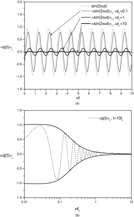
Figure 1a shows the example function and its evolving averages at different local average times. Clearly, we can see that the frequencies of the averaging results remain the same as the example function, but the amplitudes and phases are very different from each other. When ϖt_L = 0.1, this function represents a low-frequency motion and its evolving average has a magnitude similar to the function. When ϖt_L = 10, this function represents a high-frequency motion and the magnitude of its evolving average is very small as compared to the function. Figure 1b shows an averaging result as a function of ϖt_L. The envelope function represents the amplitude of the averages. Clearly we can see, with a small ϖt_L, the amplitude of the average has little change from the example function, while with a large ϖt_L, the amplitude of the average approaches zero, indicating that low-frequency function will remain in the evolving average and high-frequency function will be suppressed.

Figure 1.

(a) The example function, q(t) = sin (2πϖt), and its evolving averages at three local average times: ϖt_L = 0.1, 1, and 10. (b) The evolving average of the example function as a function of the frequency. The envelope curves show the amplitude as a function of ϖt_L. At small ϖt_L, which corresponds to a low frequency, the amplitude is approaching 1, very similar to that of the example function, while at a large ϖt_L, which corresponds to a high frequency, the amplitude approaches 0.

With the evolving averaging, many low-frequency properties can be obtained in molecular simulation. For example, low-frequency forces:

$${\tilde{\mathbf{f}}}_i\left(t\right)=\left(1-\frac{\delta t}{t_L}\right){\tilde{\mathbf{f}}}_i(t-\delta t)+\frac{\delta t}{t_L}{\mathbf{f}}_i\left(t\right);$$

low-frequency momentums:

$${\tilde{\mathbf{p}}}_i\left(t\right)=\left(1-\frac{\delta t}{t_L}\right){\tilde{\mathbf{p}}}_i(t-\delta t)+\frac{\delta t}{t_L}{\mathbf{p}}_i\left(t\right);$$

and low-frequency potential energies:

$${\tilde{E}}_p\left(t\right)=\left(1-\frac{\delta t}{t_L}\right){\tilde{E}}_p(t-\delta t)+\frac{\delta t}{t_L}{E}_p\left(t\right).$$

We can calculate some derived low-frequency quantities from these low-frequency properties, such as low-frequency kinetic energies:

$${\tilde{E}}_k=\frac{1}{2}\sum _i\frac{{\tilde{p}}_i^2}{m_i},$$ (5)

and low-frequency temperature:

$$\tilde{T}=\frac{{\tilde{E}}_k}{N_{\mathrm{DF}}k}.$$ (6)

Here, N_DF is the number of degree of freedom and k is the Boltzmann constant.

The self-guided Langevin dynamics

Langevin dynamics (LD) is based on the following equation of motion:

$${\dot{\mathbf{p}}}_i={\mathbf{f}}_i-{\gamma }_i{\mathbf{p}}_i+{\mathbf{R}}_i,$$ (7)

where ${\dot{\mathbf{p}}}_i$ and f_i are the time derivative of the momentum and the interaction force of particle i, respectively. R_i is a random force, which is related to mass, m_i, the collision frequency, γ_i, and simulation temperature, T, by the following equation:

$$⟨{\mathbf{R}}_i\left(0\right){\mathbf{R}}_i\left(t\right)⟩=2m_{i}kT{\gamma }_i\delta \left(t\right).$$ (8)

By adding a guiding force, we obtain the equation of motion for SGLD:¹

$${\dot{\mathbf{p}}}_i={\mathbf{f}}_i+{\mathbf{g}}_i-{\gamma }_i{\mathbf{p}}_i+{\mathbf{R}}_i,$$ (9)

g_i is called the guiding force and is calculated based on the low-frequency momentum:

$${\mathbf{g}}_i\left(t\right)={\lambda }_i{\gamma }_i\left({\tilde{\mathbf{p}}}_i\left(t\right)-\xi {\mathbf{p}}_i\left(t\right)\right).$$ (10)

Here, λ_i is the guiding factor. The parameter, ξ, is an energy conservation factor to cancel the energy input from the guiding force,

$$\sum _i{\mathbf{g}}_i·{\dot{\mathbf{r}}}_i=\sum _i{\lambda }_i{\gamma }_i{\tilde{\mathbf{p}}}_i·{\dot{\mathbf{r}}}_i-\xi \sum _i{\lambda }_i{\gamma }_i{\mathbf{p}}_i·{\dot{\mathbf{r}}}_i=0.$$ (11)

Here, the summation runs over all particles in a simulation system. From Eq. 11 we have

$$\xi =\frac{{\sum }_i{\lambda }_i{\gamma }_i{\tilde{\mathbf{p}}}_i·{\dot{\mathbf{r}}}_i}{{\sum }_i{\lambda }_i{\gamma }_i{\mathbf{p}}_i·{\dot{\mathbf{r}}}_i}.$$ (12)

Conformational distribution in SGLD

The guiding force in a SGLD simulation is designed to accelerate the low-frequency motion so the conformational search efficiency can be enhanced. It has two types of effects on a simulation system. First, the guiding force enhances the low-frequency motion as measured by the increase in the low-frequency temperature, and also it reduces the high-frequency motion due to the energy conservation force that comes with the guiding force [see Eq. 10]. Second, the guiding force produces a bias in the energy surface. Based on these two effects, the partition function of a SGLD ensemble is split into low-frequency and high-frequency parts:

$${\Theta }_{\mathrm{SGLD}}=\sum \Omega \exp \left(-\frac{{\lambda }_{\mathrm{lf}}{\tilde{E}}_p}{k{T}_{\mathrm{lf}}}-\frac{{\lambda }_{\mathrm{hf}}(E_p-{\tilde{E}}_p)}{k{T}_{\mathrm{hf}}}\right).$$ (13)

Here, λ_lf is called the low-frequency energy factor, describing the energy bias in the low-frequency energy surface, ${\tilde{E}}_p$, and λ_hf is the high-frequency energy factor, describing the energy bias in the high-frequency energy surface, $E_p-{\tilde{E}}_p$. The low-frequency and high-frequency energy surfaces under the guiding effect are ${\lambda }_{\mathrm{lf}}{\tilde{E}}_p$ and ${\lambda }_{\mathrm{hf}}(E_p-{\tilde{E}}_p)$, respectively. T_lf and T_hf are the effective temperatures in low-frequency and high-frequency conformational spaces, respectively. In normal conditions without the guiding forces (λ = 0), λ_lf = λ_hf = 1, and T_lf = T_hf = T, we have:

$$\begin{array}{ccc}\hfill {\Theta }_{\mathrm{SGLD}}(\lambda =0)& =& \sum \Omega \exp \left(-\frac{{\tilde{E}}_p}{kT}-\frac{(E_p-{\tilde{E}}_p)}{kT}\right)\hfill \\ & =& \sum \Omega \exp \left(-\frac{E_p}{kT}\right)={\Theta }_{\mathrm{LD}}.\hfill \end{array}$$

In the low-frequency conformational space, the equation of motion can be expressed as an evolving averaging of Eq. 9:

$${\dot{\tilde{\mathbf{p}}}}_i={\tilde{\mathbf{f}}}_i+{\tilde{\mathbf{g}}}_i-{\gamma }_i{\tilde{\mathbf{p}}}_i+{\tilde{\mathbf{R}}}_i.$$ (14)

The low-frequency energy factor, λ_lf, can be calculated according to the projection of the total low-frequency force in the direction of the low-frequency forces:

$${\lambda }_{\mathrm{lf}}=\frac{〈{\sum }_i({\tilde{\mathbf{f}}}_i+{\tilde{\mathbf{g}}}_i-{\gamma }_i{\tilde{\mathbf{p}}}_i){\tilde{\mathbf{f}}}_i〉}{〈{\sum }_i{\tilde{\mathbf{f}}}_i{\tilde{\mathbf{f}}}_i〉}.$$ (15)

Similarly, in the high-frequency conformational space, the equation of motion can be expressed as the difference between the instantaneous motion, Eq. 9, and the low-frequency motion Eq. 14:

$${\dot{\mathbf{p}}}_i-{\dot{\tilde{\mathbf{p}}}}_i={\mathbf{f}}_i-{\tilde{\mathbf{f}}}_i+{\mathbf{g}}_i-{\tilde{\mathbf{g}}}_i-{\gamma }_i({\mathbf{p}}_i-{\tilde{\mathbf{p}}}_i)+{\mathbf{R}}_i-{\tilde{\mathbf{R}}}_i.$$ (16)

The high-frequency energy factor, λ_hf, can be calculated according to the projection of the total high-frequency force in the direction of the high-frequency forces:

$${\lambda }_{\mathrm{hf}}=\frac{〈{\sum }_i\left({\mathbf{f}}_i-{\tilde{\mathbf{f}}}_i+{\mathbf{g}}_i-{\tilde{\mathbf{g}}}_i-{\gamma }_i({\mathbf{p}}_i-{\tilde{\mathbf{p}}}_i)\right)({\mathbf{f}}_i-{\tilde{\mathbf{f}}}_i)〉}{〈{\sum }_i({\mathbf{f}}_i-{\tilde{\mathbf{f}}}_i)({\mathbf{f}}_i-{\tilde{\mathbf{f}}}_i)〉}.$$ (17)

Next, let us examine the guiding force effect on low-frequency and high-frequency motions. Under the guiding force, a system experiences an enhanced motion in the low-frequency conformational space. This motion in the low-frequency conformational space can be measured by the low-frequency temperature [see Eq. 6]. It is reasonable to assume that the effective temperature in the local frequency conformational space is proportional to the low-frequency temperature:

$$T_{\mathrm{lf}}=C_{\mathrm{lf}}\tilde{T}.$$

And the effective temperature in the high-frequency conformational space is proportional to the high-frequency temperature:

$$T_{\mathrm{hf}}=C_{\mathrm{hf}}(T-\tilde{T}).$$

The proportional constants can be estimated from a LD simulation or a SGLD simulation without the guiding forces (λ = 0), where T_lf = T_hf = T:

$$C_{\mathrm{lf}}=\frac{T}{{\tilde{T}}_0},$$

$$C_{\mathrm{hf}}=\frac{T}{T-{\tilde{T}}_0}.$$

Here, ${\tilde{T}}_0$ is the low-frequency temperature when λ = 0 and is called the reference low-frequency temperature. Based on the definition, we know ${\tilde{T}}_0$ depends on the simulation condition and the local average time, t_L. Therefore, the partition function of a SGLD simulation can be written as

$${\Theta }_{\mathrm{SGLD}}=\sum \Omega \exp \left(-\frac{{\lambda }_{\mathrm{lf}}{\tilde{T}}_0}{\tilde{T}}\frac{{\tilde{E}}_p}{kT}-\frac{{\lambda }_{\mathrm{hf}}(T-{\tilde{T}}_0)}{T-\tilde{T}}\frac{E_p-{\tilde{E}}_p}{kT}\right).$$ (18)

To utilize Eq. 18, in addition to λ_lf, λ_hf, ${\tilde{E}}_p,$ and $\tilde{T}$ from a SGLD simulation, we also need ${\tilde{T}}_0$ from a LD simulation or a SGLD simulation with λ = 0. To avoid this burden, we propose the following way to estimate ${\tilde{T}}_0$ directly from the same SGLD simulation.

The low-frequency motion, Eq. 14, corresponds to a Langevin dynamics in a low-frequency conformational space and can be rewritten to a Langevin dynamics form:

$${\dot{\tilde{\mathbf{p}}}}_i={\tilde{\mathbf{f}}}_i-{\chi }_{\mathrm{lf}}{\gamma }_i{\tilde{\mathbf{p}}}_i+{\tilde{\mathbf{R}}}_i.$$ (19)

Equation 19 corresponds to a Langevin dynamics with a collision frequency of χ_lfγ_i. The factor, χ_lf, is called the low-frequency collision factor and can be calculated by the following equation:

$${\chi }_{\mathrm{lf}}=\frac{{\sum }_i({\gamma }_i{\tilde{\mathbf{p}}}_i-{\tilde{\mathbf{g}}}_i){\gamma }_i{\tilde{\mathbf{p}}}_i}{{\sum }_i{\gamma }_i^2{\tilde{\mathbf{p}}}_i{\tilde{\mathbf{p}}}_i}.$$ (20)

Based on the Langevin dynamics relation, Eq. 8, with a given distribution of random forces, the product of temperature and collision frequency is a constant:

$$T{\gamma }_i=\frac{⟨{\mathbf{R}}_i\left(0\right){\mathbf{R}}_i\left(t\right)⟩}{2m_{i}k\delta \left(t\right)}.$$ (21)

The reference low-frequency temperature, ${\tilde{T}}_0$, corresponds to the low-frequency temperature at a collision frequency of γ_i, while the low-frequency temperature in a SGLD simulation, $\tilde{T}$, corresponds to that at the collision frequency of χ_lfγ_i. Because the guiding force does not affect the random force, from Eq. 21, we have

$${\tilde{T}}_0=\tilde{T}{\chi }_{\mathrm{lf}}.$$ (22)

Equation 22 provides a way to estimate ${\tilde{T}}_0$ from $\tilde{T}$, which can be calculated directly in a SGLD simulation according to Eq. 6. Therefore, the partition function can be approximated as

$$\begin{array}{c}\hfill {\Theta }_{\mathrm{SGLD}}\approx \sum \Omega \exp \left(-{\lambda }_{\mathrm{lf}}{\chi }_{\mathrm{lf}}\frac{{\tilde{E}}_p}{kT}-{\lambda }_{\mathrm{hf}}\frac{T-{\chi }_{\mathrm{lf}}\tilde{T}}{T-\tilde{T}}\frac{E_p-{\tilde{E}}_p}{kT}\right).\end{array}$$ (23)

In summary, at a given temperature, T, the guiding force produces the following effects in both low and high-frequency conformational spaces:

• a.In the low-frequency conformational space, the low-frequency energy surface, ${\tilde{E}}_p$, is modified by a factor of λ_lf. The effective temperature is changed from T to $T_{\mathrm{lf}}=\frac{\tilde{T}}{{\tilde{T}}_0}T=\frac{T}{{\chi }_{\mathrm{lf}}}$.
• b.In the high-frequency conformational space, the high-frequency energy surface, $E_p-{\tilde{E}}_p$, is modified by a factor of λ_hf. The effective temperature is changed from T to $T_{\mathrm{hf}}=\frac{T-\tilde{T}}{T-{\tilde{T}}_0}T=\frac{T-\tilde{T}}{T-{\chi }_{\mathrm{lf}}\tilde{T}}T$.

The partition function of a canonical ensemble from a LD simulation can be related to that of a SGLD ensemble by the following equation:

$$\begin{array}{ccc}\hfill {\Theta }_{\mathrm{LD}}& =& \sum \Omega \exp \left(-\frac{{\tilde{E}}_p}{kT}-\frac{E_p-{\tilde{E}}_p}{kT}\right)\hfill \\ & =& \sum \Omega \exp \left(-{\lambda }_{\mathrm{lf}}\frac{{\tilde{T}}_0}{\tilde{T}}\frac{{\tilde{E}}_p}{kT}-{\lambda }_{\mathrm{hf}}\frac{(T-{\tilde{T}}_0)}{(T-\tilde{T})}\frac{E_p-{\tilde{E}}_p}{kT}\right)\hfill \\ & & \times \exp (\left({\lambda }_{lf}\frac{{\tilde{T}}_0}{\tilde{T}}-1\right)\frac{{\tilde{E}}_p}{kT}+\left({\lambda }_{\mathrm{hf}}\frac{(T-{\tilde{T}}_0)}{(T-\tilde{T})}-1\right)\hfill \\ & & \times \frac{E_p-{\tilde{E}}_p}{kT}).\hfill \\ & =& {\Theta }_{\mathrm{SGLD}}{⟨w_{\mathrm{SGLD}}⟩}_{\mathrm{SGLD}}\hfill \end{array}$$ (24)

Here, w_SGLD is called the SGLD weighting factor:

$$\begin{array}{ccc}\hfill w_{\mathrm{SGLD}}& =& \exp (\left({\lambda }_{\mathrm{lf}}\frac{{\tilde{T}}_0}{\tilde{T}}-1\right)\frac{{\tilde{E}}_p}{kT}+\left({\lambda }_{\mathrm{hf}}\frac{T-{\tilde{T}}_0}{T-\tilde{T}}-1\right)\hfill \\ & & \times \frac{E_p-{\tilde{E}}_p}{kT})\hfill \\ & \approx & \exp (\left({\lambda }_{\mathrm{lf}}{\chi }_{\mathrm{lf}}-1\right)\frac{{\tilde{E}}_p}{kT}\hfill \\ & & +\left({\lambda }_{\mathrm{hf}}\frac{T-{\chi }_{\mathrm{lf}}\tilde{T}}{T-\tilde{T}}-1\right)\frac{E_p-{\tilde{E}}_p}{kT}).\hfill \end{array}$$ (25)

To calculate the weighting factor according to Eq. 25, we need E_p and ${\tilde{E}}_p$ for each conformation, as well as $\tilde{T}$, λ_lf, λ_hf, and χ_lf from the SGLD simulation. Once we have the weighting factor, any ensemble average, ⟨A ⟩, can be calculated in a SGLD simulation as

$$⟨A⟩=\frac{{⟨A{w}_{\mathrm{SGLD}}⟩}_{\mathrm{SGLD}}}{{⟨w_{\mathrm{SGLD}}⟩}_{\mathrm{SGLD}}}.$$ (26)

The self-guiding temperature

In SGLD simulations, the guiding factor, λ, is an input parameter whose value is often hard to decide for its lack of physical meaning. For the convenience in describing the conformational search ability of a SGLD simulation, we define a so called self-guiding temperature, T_sg, based on the effective temperatures in the low and high-frequency conformational spaces:

$$T_{\mathrm{sg}}=\frac{T_{\mathrm{lf}}}{T_{\mathrm{hf}}}T=\frac{\tilde{T}(T-{\tilde{T}}_0)}{{\tilde{T}}_0(T-\tilde{T})}T.$$ (27)

The self-guiding temperature, T_sg, provides a rough measure of the conformational searching ability in the unit of temperature. A SGLD simulation with a self-guiding temperature of T_sg has a conformational search ability comparable to that in a high-temperature simulation at the temperature of T_sg. As can be seen from Eq. 27, for a LD simulation, $\tilde{T}={\tilde{T}}_0$, we have T_sg = T. For a SGLD simulation with λ > 0, we have $\tilde{T}>{\tilde{T}}_0$ and T_sg > T, and with λ < 0, , we have $\tilde{T}<{\tilde{T}}_0$ and T_sg < T. T_sg can be used as a guidance for choosing λ. For example, it is reasonable to choose a λ that produces T_sg = 2T. However, when λ is large and T_sg is too large as compared to T, it is difficult to obtain accurate canonical ensemble through reweighting with Eqs. 25, 26. Therefore, λ should be chosen to balance the acceleration of conformational search and the accuracy in converting conformational distribution.

SIMULATION DETAILS

To demonstrate the ensemble distribution in SGLD simulations and the conversion to canonical ensembles, we report the results for several simple systems. A leap-frog Verlet algorithm for the SGLD simulation has been implemented into CHARMM (Refs. ^{6, 7}), version 36 and is described in the Appendix. Because a SGLD simulation involves extra calculation only in the propagation of the equations of motion as compared to a normal LD simulation, the cost of a SGLD simulation is almost identical to a LD simulation for the same number of time steps. SGLD simulations do require additional memory because of the need to store the guiding forces, as well as some arrays for the weighting factor calculation.

RESULTS AND DISCUSSIONS

Through the three model systems presented here we demonstrate three points: (1) effect of guiding forces on conformational search, (2) effect of guiding forces on conformational distribution, and (3) conversion from SGLD conformational distributions to LD conformational distributions.

The skewed double well system

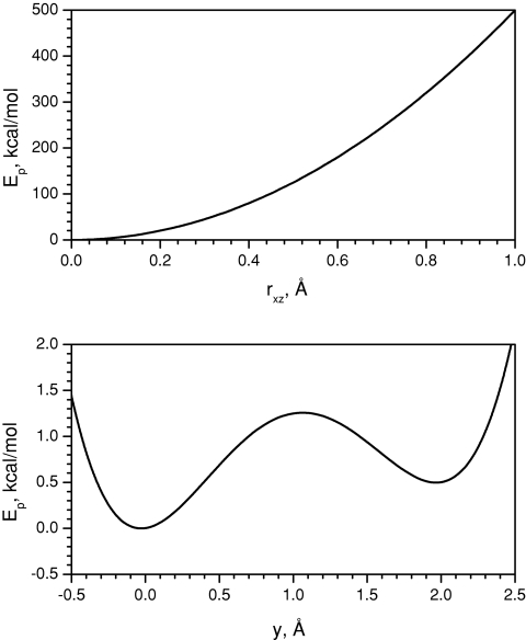
A skewed double well system represents the simplest nonsymmetric system with an energy barrier to cross. This system has only one particle and the particle moves on a fixed energy surface. This energy surface is designed in such a way that it restricts the particle to move near the y-axis with two energy minimums of different depths along the y-axis. Such a design forces the particle to have a high-frequency motion in the x–z direction and a low-frequency motion in the y direction. The potential profiles along the y-axis and across the y-axis are shown in Fig. 2. The potential function (in kcal∕mol) is

$${\varepsilon }_p=500(x^2+z^2)+y^2{(y-2)}^2+0.25y.$$ (28)

An argon atom was used to represent the particle. Simulations were carried out at 80 K with a local average time, t_L = 0.2 ps. A time step of 1 fs was used and the simulation length was 100 ns for each simulation.

Figure 2.

The skewed double well potential along the y-axis (lower panel) when r_xz = 0 and perpendicular to the y-axis (upper panel) when y = 0.

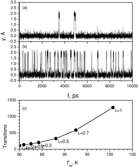
Figure 3 shows two trajectories in y coordinates, one in a LD simulation [Fig. 3a] and the other in a SGLD simulation with λ = 1 [Fig. 3b]. Clearly, the transition between the two wells at y = 0 Å and y = 2 Å are more frequent in the SGLD simulation than that in the LD simulation, demonstrating an enhanced energy barrier overcoming ability in the SGLD simulation. Figure 3c shows the number of transitions as a function of T_sg. When λ increases, T_sg increases, so does the transitions between the wells. At λ = 1, T_sg = 100.7 K, the transitions increases by about 10 times more than the transitions in a LD simulation (i.e., λ = 0 and T_sg = T = 80 K). This result demonstrates the dramatic enhancement in the energy barrier crossing ability.

Figure 3.

Transitions of the particle in the double well system. (a) Trajectory in the LD simulation; (b) Trajectory in the SGLD simulation with λ = 1 where T_sg = 100.7 K. (c) Transition number as a function of the self-guiding temperature, T_sg. The collision frequency is 10∕ps and temperature is 80 K.

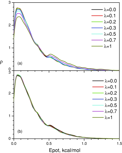
Figure 4a shows the potential energy distribution in the SGLD simulations. As λ increases, the distribution decreases in the low-energy region and increases in the high-energy region. Figure 4b shows the weighted energy distributions. Clearly, all curves converge fairly well to the one with λ = 0, demonstrating that the weighting scheme can convert the SGLD distributions to the canonical energy distribution with a reasonable degree of accuracy.

Figure 4.

The energy distributions of the double well system in the SGLD simulations: (a) unweighted; (b) weighted. The collision frequency is 10∕ps and temperature is 80 K.

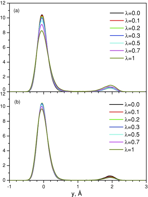
To further examine the guiding effect on the conformational distribution, we plot the conformational density as a function of the y coordinate in Fig. 5. Figure 5a shows the distributions at different guiding factors. There are two peaks with different heights, corresponding to the skewed double wells. Examining the peak heights at different λ, we can see that as λ increases, the left peak (the higher peak) decreases, while the right peak (the lower peak) grows. Figure 5b shows the weighted conformational distribution. All distributions converge fairly well to the one with λ = 0. This result again validates the reweighting scheme.

Figure 5.

The y-coordinate distributions of the double well system in the SGLD simulations: (a) unweighted; (b) weighted. The collision frequency is 10∕ps and temperature is 80 K.

It should be noted that the reweighting scheme, Eqs. 24, 25, 26, is based on the first order perturbation approximation and is limited to small difference in conformational distribution. As can be seen in Fig. 5b, when the guiding factor is large, the deviation from the LD distribution increases. Further increasing the guiding factor will make the reweighting hard to converge.

Argon fluid

Argon liquid represents a typical homogeneous system. It is a convenient system to examine ensemble average properties. Argon atoms were described by the Lennard-Jones 6–12 potentials with ɛ = 119.8 K and σ = 3.405 Å. In this example system, 500 argon atoms were placed in a cubic periodic box (28.53 × 28.53 × 28.53 ų). A time step of 1 fs was used for all simulations. The simulation length was 10 ns for each simulation. The temperature was set to 100 K except otherwise noted. Nonbonded interactions were calculated using the following rationalized polynomial 3D isotropic periodic sum (IPS) potentials.^{6, 8}

Lennard-Jones IPS potentials:

$${\varepsilon }_{\mathrm{disp}}^{\mathrm{IPS}}(r,R)=\left\{\begin{array}{cc}{\displaystyle \begin{array}{c}{\displaystyle -\frac{C_{ij}}{r^6}-\frac{C_{ij}}{R^6}\left({\displaystyle \frac{1341}{3064}+\frac{77}{141}{\left({\displaystyle \frac{r}{R}}\right)}^2+\frac{61}{141}{\left({\displaystyle \frac{r}{R}}\right)}^4+\frac{56}{141}{\left({\displaystyle \frac{r}{R}}\right)}^8}\right)}\hfill \\ \begin{array}{c}\\ 0\hfill \end{array}\hfill \end{array}}\hfill & \begin{array}{c}\begin{array}{c}\\ r\le R\hfill \end{array}\hfill \\ \begin{array}{c}\\ r>R\hfill \end{array}\hfill \end{array}\hfill \end{array}\right.,$$ (29)

$${\varepsilon }_{\mathrm{rep}}^{\mathrm{IPS}}(r,R)=\left\{\begin{array}{cc}\begin{array}{c}{\displaystyle \frac{A_{ij}}{r^{12}}+\frac{A_{ij}}{R^{12}}\left({\displaystyle \frac{23}{3620}+\frac{8}{151}{\left({\displaystyle \frac{r}{R}}\right)}^2+\frac{66}{151}{\left({\displaystyle \frac{r}{R}}\right)}^6+\frac{100}{151}{\left({\displaystyle \frac{r}{R}}\right)}^{10}}\right)}\hfill \\ \begin{array}{c}\\ 0\hfill \end{array}\hfill \end{array}& \begin{array}{c}\begin{array}{c}\\ r\le R\hfill \end{array}\\ \begin{array}{c}\\ r>R\hfill \end{array}\end{array}\end{array}\right..$$ (30)

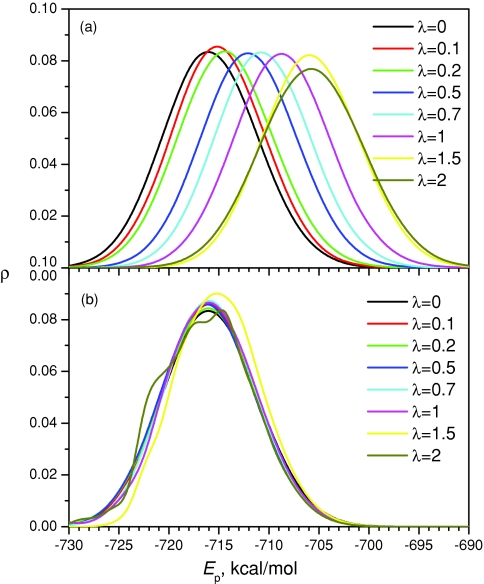
Figure 6a shows the potential energy distributions in the SGLD simulations at different guiding factors. Clearly, the energy distribution changes with the guiding factor. When applying the weighting scheme, the energy distribution converges together [Fig. 6b], except when λ > 1 where numerical convergence becomes a problem due to the large difference in the conformational distribution. As shown in Eq. 25, the weighting factor varies exponentially with the energies. The weighting scheme will converge poorly if the major distribution to be calculated is not properly sampled in the simulation. Note that if the simulation length is significantly increased, convergence would improve for larger λ values. About the precision of reweighting in simulations, Shen and Hamelberg has a more thorough analysis.⁹

Figure 6.

The energy distributions of the argon liquid in the SGLD simulations at 100 K: (a) unweighted; (b) weighted. The collision frequency is 1∕ps.

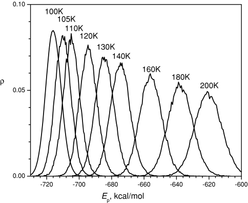
Many enhanced sampling techniques come with a certain alteration of the conformational distribution. Increasing temperature is a commonly used approach to speed up a conformational search. However, the change in conformational distribution due to a rise in temperature is significant. Figure 7 shows the potential energy distributions of the argon fluid from LD simulations at different temperatures. Clearly we can see potential energies shift toward high energies when temperature increases. Comparing the distributions at 100 and 140 K, there is little conformation shared by both distributions. In other words, a temperature increase can speed up simulations but most of the conformations searched at 140 K are of little importance to the distribution at 100 K, which makes a reweighting formula to correct for the effects of higher temperature difficult to converge.

Figure 7.

The energy distributions of the argon liquid in the LD simulations at different temperatures (as labeled). The collision frequency is 1∕ps.

Obviously, the potential energy shifts up in a much smaller scale in SGLD simulations [Fig. 6a] than that when raising the temperature. Comparing Figs. 6a, 7, we can see that the energy deviations due to the guiding effect is much smaller than the deviation due to the temperature increase.

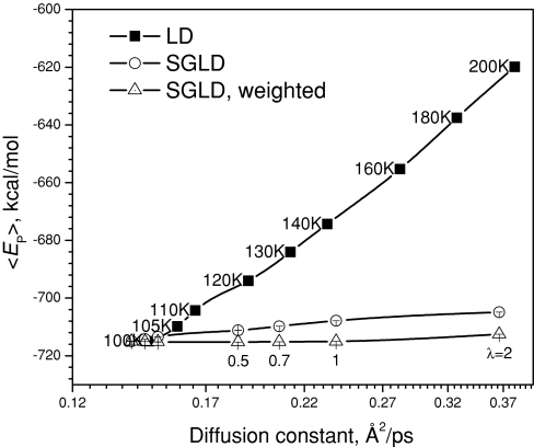
To quantitatively compare the SGLD and high-temperature LD simulations, we plot the average potential energies against diffusion constants in Fig. 8. Diffusion constants measure the conformational change in the slowest frequency and can be a good measurement of the conformational search efficiency. The diffusion constants were calculated with a fixed center of mass to avoid any exaggeration due to the motion of the center of mass. As can be seen from Fig. 8, SGLD increases diffusion constants with much smaller energy deviations than LD simulations at elevated temperatures. This plot tells us that SGLD can speed up conformational searches with little change in conformational distribution, while high-temperature LD simulation speeds up conformational search, but searches a conformational space far away from that at the temperature of interest.

Figure 8.

Average potential energies vs diffusion constants for the argon liquid in the LD simulations at different temperatures (as labeled) and in the SGLD simulations at different guiding factors (as labeled). The collision frequency is 1∕ps. The SGLD simulations were performed at 100 K.

The weighted average potential energies are also plotted against diffusion constants in Fig. 8. For SGLD, the weighted potential energy is very flat against diffusion constant. In other words, through the weighting procedure, SGLD can speed up conformational searches and produce accurate conformational distribution.

Alanine dipeptide

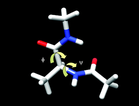
The Alanine dipeptide is perhaps the simplest and the most well studied molecule that is relevant to proteins. Figure 9 shows one conformation of an alanine dipeptide. The conformation of this molecule is mainly characterized by two dihedral angles, ϕ: CT–N–Cα–C and ψ: N–Cα–C–NT. The CHARMM all-atom force field⁶ was used to describe the interactions. Here, we used a distance-dependent dielectric constant of 4r to represent solvent screening effect to simplify the example. The cutoff distance is set to 100 Å to avoid any cutoff effect in the nonbonded interaction calculation within this small molecule.

Figure 9.

A conformation of an alanine dipeptide. Chemical bonds are shown as sticks. Oxygen and nitrogen atoms are shown as red and blue, respectively. Two backbone dihedral angles, ϕ and ψ, are marked by arrows.

All simulations were performed with a time step of 2 fs and SHAKE algorithm¹⁰ was employed to fix the bond lengths. Each simulation was 200 ns in length and conformations of every 2 ps were saved for postanalysis. The SGLD simulations were performed with a local average time of t_L = 0.2 ps and a temperature of 300 K.

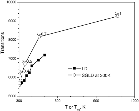
To demonstrate the conformational search of SGLD simulations, we performed high-temperature LD simulations, as well as SGLD simulations with different guiding factors for the alanine dipeptide. To quantitatively describe the conformational search of this peptide, we calculated the transition rate for the dihedral angles, (ϕ, ψ) to transfer from one local minimum at (–90°,–70°) to another local minimum at (–90°, 170°). One transfer is counted when (ϕ, ψ) is changing from within 40° of one local minimum to within 40° of the other local minimum.

Figure 10 shows the transition rate in the LD simulations against the simulation temperature and in the SGLD simulations against the self-guiding temperature. The self-guiding temperature is defined to reflect the conformational searching ability [Eq. 27] of a SGLD simulation so that users can have a rough idea of how much conformational search ability has been achieved. As can be seen from Fig. 10, the transition rate increases with the temperature or the self-guiding temperature in a similar trend. The transition rates of SGLD simulations is somewhat higher than that of the LD simulations at the temperature of T_sg, indicating T_sg somewhat underestimates the conformational searching ability of the SGLD simulations in this case. Figure 10 shows that the SGLD simulations at guiding factors of 0.2, 0.5, and 1 have self-guiding temperatures of 346, 458, and 1067 K, respectively, indicating that the conformational search abilities of these simulations are comparable to that of high-temperature LD simulations at 346, 458, and 1067 K, respectively. It is clear that SGLD simulations have increased the conformational search ability dramatically.

Figure 10.

Conformational transitions of the alanine dipeptide as a function of temperature in the LD simulations and as a function of the self-guiding temperature, T_sg, in the SGLD simulations. The self-guiding temperature, T_sg, defined by Eq. 27, reflects the conformational searching ability that is comparable to a high-temperature simulation at T = T_sg. The collision frequency is γ = 10∕ps. The SGLD simulations were performed at 300 K.

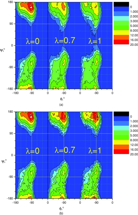
To examine the reweighting scheme in a multidimensional distribution, we plot the ϕ−ψ dihedral angle distributions from the LD and SGLD simulations in Fig. 11. Before reweighting, as shown in Fig. 11a, SGLD simulations have lower peak heights and broader baselines than the LD simulation. This result indicates that the dramatical acceleration in conformational search accompanies a change in conformational distribution. An increase in the guiding factor, λ, results in an increase in the self-guiding temperatures (Fig. 10), and as a result, the system experiences an enhanced motion in the low-frequency conformational space. This enhanced motion increases conformational search ability, but also flattens the conformational distribution. As the guiding factor increases, the high peaks become lower and the valleys become shallower. After reweighting, as can be seen in Fig. 11b, the peak heights and the baseline broadness of the SGLD results are quite similar to that of the LD simulation. This result again validates the weighting scheme. Obviously, the reweighting result is noisier at a larger guiding factor. A smaller guiding factor will help reduce the reweighting noise, but have a weaker conformational search ability. Therefore, the guiding factor should be set to have enough conformational search ability while allowing a reweighting of acceptable accuracy.

Figure 11.

(a) ϕ−ψ distributions of the alanine dipeptide in the LD (λ = 0) and SGLD simulations at λ = 0.7 and λ = 1 before reweighting. The collision frequency is γ = 10∕ps. The SGLD simulations were performed at 300 K. (b) ϕ−ψ distributions of the alanine dipeptide in the LD (λ = 0) and SGLD simulations at λ = 0.7 and λ = 1 after reweighting. The collision frequency is γ = 10∕ps. The SGLD simulations were performed at 300 K.

CONCLUSIONS

The conformational distribution from SGLD simulation is quantitatively described through the low-frequency and high-frequency properties. This provides a way to convert conformational distributions from SGLD simulations to canonical ensemble distributions. Through this work, the SGLD simulation method can be used not only to achieve a dramatically enhanced conformational search, but also to produce an accurate conformational distribution. This understanding of the SGLD conformational distribution provides a sound theoretical basis for further development and application of this method.

APPENDIX: SGLD SIMULATION ALGORITHM

To help understand how to calculate ensemble averages from SGLD simulations, we describe a leap-frog Verlet SGLD simulation algorithm below.

• (i)Initiate low-frequency variables: ${\tilde{E}}_p\left(0\right)=E_p\left(0\right)$, ${\tilde{\mathbf{f}}}_i\left(0\right)=0$, ${\tilde{\mathbf{p}}}_i\left(0\right)=0$, and ${\tilde{\mathbf{g}}}_i\left(0\right)=0$.
• (ii)
  At time step, t, calculate interaction forces, f_i(t), random forces, R_i(t), and the uncorrected guiding forces, ${{\mathbf{g}}^{\prime }}_i\left(t\right)={\lambda }_i{\gamma }_i{\tilde{\mathbf{p}}}_i\left(t\right)$. The interaction forces, f_i(t), must include any constraint force as described later. Random forces, R_i(t), are generated from a Gaussian distribution with zero mean:

  $$\rho \left({\mathbf{R}}_i\right)=\frac{1}{\sqrt{4\pi {\gamma }_i{m}_{i}kT}}{e}^{-\frac{{\mathbf{R}}_i^2}{4{\gamma }_i{m}_{i}kT}}.$$ (A1)

  The low-frequency momentum is calculated using the momentum in the previous half step, ${\mathbf{p}}_i(t-\frac{\delta t}{2})$:

  $${\tilde{\mathbf{p}}}_i\left(t\right)=\left(1-\frac{\delta t}{t_L}\right){\tilde{\mathbf{p}}}_i(t-\delta t)+\frac{\delta t}{t_L}{\mathbf{p}}_i\left(t-\frac{\delta t}{2}\right).$$ (A2)
• (iii)
  Calculate the energy conservation factor, ξ. The half step velocity, ${\dot{\mathbf{r}}}_i\left(t\right)$, can be expressed in the following form:

  $$\begin{array}{ccc}\hfill {\dot{\mathbf{r}}}_i\left(t\right)& =& {\dot{\mathbf{r}}}_i\left(t-\frac{\delta t}{2}\right)+\frac{\delta t}{2m_i}\left({\mathbf{f}}_i\left(t\right)+{{\mathbf{g}}^{\prime }}_i\left(t\right)+{\mathbf{R}}_i\left(t\right)\right)\hfill \\ & & -\frac{\delta t}{2}({\gamma }_i+\xi {\lambda }_i{\gamma }_i){\dot{\mathbf{r}}}_i\left(t\right);\hfill \end{array}$$ (A3)

  calculate the friction-free velocity at the half step:

  $${\dot{{\mathbf{r}}^{\prime }}}_i\left(t\right)={\dot{\mathbf{r}}}_i\left(t-\frac{\delta t}{2}\right)+\frac{\delta t}{2m_i}\left({\mathbf{f}}_i\left(t\right)+{{\mathbf{g}}^{\prime }}_i\left(t\right)+{\mathbf{R}}_i\left(t\right)\right).$$ (A4)

  From Eqs. A3, A4, we have

  $$\begin{array}{ccc}\hfill {\dot{\mathbf{r}}}_i\left(t\right)& =& {\displaystyle \frac{{\dot{{\mathbf{r}}^{\prime }}}_i\left(t\right)}{{\displaystyle 1+\frac{(1+\xi {\lambda }_i){\gamma }_i\delta t}{2}}}\approx \frac{{\dot{{\mathbf{r}}^{\prime }}}_i\left(t\right)}{{\displaystyle 1+\frac{{\gamma }_i\delta t}{2}}}}\hfill \\ & & {\displaystyle -\frac{{\dot{{\mathbf{r}}^{\prime }}}_i\left(t\right)}{{\left({\displaystyle 1+\frac{{\gamma }_i\delta t}{2}}\right)}^2}\frac{\xi {\lambda }_i{\gamma }_i\delta t}{2}.}\hfill \end{array}$$ (A5)

  Based on the energy conservation relation, Eq. 11, and neglect the higher power term of ξ, we can solve the energy conservation factor:

  $${\displaystyle \xi =\frac{{\displaystyle \sum _i^N{\lambda }_i{\gamma }_i{\tilde{\mathbf{p}}}_i\left(t\right){\dot{{\mathbf{r}}^{\prime }}}_i\left(t\right){\left({\displaystyle 1+\frac{{\gamma }_i\delta t}{2}}\right)}^{-1}}}{{\displaystyle \sum _i^N{\displaystyle {\lambda }_i{\gamma }_i{m}_i{\dot{{\mathbf{r}}^{\prime }}}_i^2\left(t\right){\left({\displaystyle 1+\frac{{\gamma }_i\delta t}{2}}\right)}^{-2}+\frac{\delta t}{2}\sum _i^N{\lambda }_i^2{\gamma }_i^2{\tilde{\mathbf{p}}}_i\left(t\right){\dot{{\mathbf{r}}^{\prime }}}_i\left(t\right){\left({\displaystyle 1+\frac{{\gamma }_i\delta t}{2}}\right)}^{-2}}}}.}$$ (A6)
  The actual guiding force is

  $$\begin{array}{ccc}\hfill {\mathbf{g}}_i\left(t\right)& =& {\lambda }_i{\gamma }_i{\tilde{\mathbf{p}}}_i\left(t\right)-\xi {\mathbf{p}}_i\left(t\right)\hfill \\ & =& {\displaystyle {\lambda }_i{\gamma }_i{\tilde{\mathbf{p}}}_i\left(t\right)-\frac{\xi m_i{\dot{{\mathbf{r}}^{\prime }}}_i\left(t\right)}{{\displaystyle 1+\frac{(1+\xi {\lambda }_i){\gamma }_i\delta t}{2}}}.}\hfill \end{array}$$ (A7)
• (iv)
  Update low-frequency variables and accumulators for the calculation of the SGLD weighting factor. Low-frequency forces:

  $${\tilde{\mathbf{f}}}_i\left(t\right)=\left(1-\frac{\delta t}{t_L}\right){\tilde{\mathbf{f}}}_i(t-\delta t)+\frac{\delta t}{t_L}{\mathbf{f}}_i\left(t\right).$$

  Low-frequency potential energy:

  $${\tilde{E}}_p\left(t\right)=\left(1-\frac{\delta t}{t_L}\right){\tilde{E}}_p(t-\delta t)+\frac{\delta t}{t_L}{E}_p\left(t\right).$$

  Low-frequency guiding forces:

  $${\tilde{\mathbf{g}}}_i\left(t\right)=\left(1-\frac{\delta t}{t_L}\right){\tilde{\mathbf{g}}}_i(t-\delta t)+\frac{\delta t}{t_L}{\mathbf{g}}_i(\left(t\right).$$

  From the low-frequency momentums we can calculate the low-frequency temperature:

  $$\tilde{T}=\frac{1}{N_{\mathrm{DF}}}\sum _i\frac{{\tilde{\mathbf{p}}}_i^2}{m_i}.$$

  Update accumulators for the collision factors and energy factors:

  $$\mathrm{FLF}=\sum _t\sum _i^N{\tilde{\mathbf{f}}}_i\left(t\right)·{\tilde{\mathbf{f}}}_i\left(t\right),$$

  $$\mathrm{FHF}=\sum _t\sum _i^N({\mathbf{f}}_i\left(t\right)-{\tilde{\mathbf{f}}}_i\left(t\right))·({\mathbf{f}}_i\left(t\right)-{\tilde{\mathbf{f}}}_i\left(t\right)),$$

  $$\mathrm{GLF}=\sum _t\sum _i^N\left({\tilde{\mathbf{g}}}_i\left(t\right)-{\gamma }_i{\tilde{\mathbf{p}}}_i\left(t\right)\right)·{\tilde{\mathbf{f}}}_i\left(t\right),$$

  $$\begin{array}{ccc}\hfill \mathrm{GHF}& =& \sum _t\sum _i^N\left({\mathbf{g}}_i\left(t\right)-{\tilde{\mathbf{g}}}_i\left(t\right)-{\gamma }_i({\mathbf{p}}_i\left(t\right)-{\tilde{\mathbf{p}}}_i\left(t\right))\right)\hfill \\ & & ·({\mathbf{f}}_i\left(t\right)-{\tilde{\mathbf{f}}}_i\left(t\right))\hfill \end{array}$$

  $$\mathrm{PPLF}=\sum _t\sum _i^N{\gamma }_i^2{\tilde{\mathbf{p}}}_i\left(t\right)·{\tilde{\mathbf{p}}}_i\left(t\right),$$

  $$\mathrm{GPLF}=\sum _t\sum _i^N{\tilde{\mathbf{g}}}_i\left(t\right)·{\gamma }_i{\tilde{\mathbf{p}}}_i\left(t\right).$$
  The collision and energy factors are calculated with the accumulators:

  $$\begin{array}{c}{\displaystyle {\lambda }_{\mathrm{lf}}=1+\frac{\mathrm{GLF}}{\mathrm{FLF}},{\lambda }_{\mathrm{hf}}=1+\frac{\mathrm{GHF}}{\mathrm{FHF}},}\\ {\displaystyle {\chi }_{\mathrm{lf}}=\frac{{\tilde{T}}_0}{\tilde{T}}=1-\frac{\mathrm{GPLF}}{\mathrm{PPLF}}.}\end{array}$$ (A8)

  When ${\tilde{T}}_0$ is available from a previous SGLD simulation with λ = 0, ${\chi }_{\mathrm{lf}}=\frac{{\tilde{T}}_0}{\tilde{T}}$ is recommended, otherwise, ${\chi }_{\mathrm{lf}}=1-\frac{\mathrm{GPLF}}{\mathrm{PPLF}}$ has to be used. The SGLD weighting factor of each conformation can be calculated as below during a simulation or in a postsimulation processing:

  $$\begin{array}{ccc}\hfill w_{\mathrm{SGLD}}& =& \exp (\left({\lambda }_{\mathrm{lf}}{\chi }_{\mathrm{lf}}-1\right)\frac{{\tilde{E}}_p-{\overline{E}}_p}{kT}\hfill \\ & & +\left({\lambda }_{\mathrm{hf}}\frac{T-{\chi }_{\mathrm{lf}}\tilde{T}}{T-\tilde{T}}-1\right)\frac{E_p-{\tilde{E}}_p}{kT}).\hfill \end{array}$$ (A9)

  In Eq. A9, the average potential energy is subtracted from the low-frequency energy to avoid overflow in calculating the exponential function. With the weighting factor, any ensemble averages can be calculated during a simulation or in a postsimulation process.
• (v)
  Advance velocities to the next half time step:

  $$\begin{array}{ccc}\hfill {\dot{\mathbf{r}}}_i\left(t+\frac{\delta t}{2}\right)& =& \left(2{\chi }_i-1\right){\dot{\mathbf{r}}}_i\left(t-\frac{\delta t}{2}\right)\hfill \\ & & +{\chi }_i\frac{\delta t}{m_i}\left({\mathbf{f}}_i\left(t\right)+{\mathbf{g}}_i\left(t\right)+{\mathbf{R}}_i\left(t\right)\right).\hfill \end{array}$$ (A10)

  Here, the scaling parameter, χ_i, is calculated as

  $${\chi }_i={\left(1+\frac{(1+\xi {\lambda }_i){\gamma }_i\delta t}{2}\right)}^{-1}.$$ (A11)

  Then advance positions to the next time step:

  $${\mathbf{r}}_i(t+\delta t)={\mathbf{r}}_i\left(t\right)+{\dot{\mathbf{r}}}_i\left(t+\frac{\delta t}{2}\right)\delta t.$$ (A12)

  If internal coordinates need to be constrained, apply constraining algorithms, such as SHAKE (Ref. ¹⁰) or semiflexible constraint dynamics,¹¹ to obtain constrained positions, ${\mathbf{r}}_i^{\mathrm{CON}}(t+\delta t)$, from r_i(t + δt). The constraint forces must be included in the low-frequency force calculation. The constraint forces are calculated by the following equation:

  $${\mathbf{f}}_i^{\mathrm{CON}}(t+\delta t)=\frac{2m_i}{\delta t^2}\left({\mathbf{r}}_i^{\mathrm{CON}}(t+\delta t)-{\mathbf{r}}_i(t+\delta t)\right).$$ (A13)
• (vi)Continue to step (ii) with t = t + δt until the end of the simulation.

References

- Wu X. and Brooks B. R., Chem. Phys. Lett. 381(3–4), 512 (2003). 10.1016/j.cplett.2003.10.013 [DOI] [Google Scholar]
- Damjanović A., García-Moreno E. B., and Brooks B. R., Proteins: Struct., Funct., Bioinf. 76(4), 1007 (2009); [DOI] [PMC free article] [PubMed] [Google Scholar]; Damjanović A., Miller B. T., Wenaus T. J., Maksimović P., Bertrand García-Moreno E., and Brooks B. R., J. Chem. Inf. Model. 48(10), 2021 (2008); [DOI] [PubMed] [Google Scholar]; Lee M. S. and Olson M. A., J. Chem. Theory Comput. 6(8), 2477 (2010); 10.1021/ct100062b [DOI] [PubMed] [Google Scholar]; Lee C. I. and Chang N. Y., Biophys. Chem. 151(1–2), 86 (2010). 10.1016/j.bpc.2010.05.002 [DOI] [PubMed] [Google Scholar]
- Damjanović A., Wu X., García-Moreno E. B., and Brooks B. R., Biophys. J. 95(9), 4091 (2008). [DOI] [PMC free article] [PubMed] [Google Scholar]
- Andricioaei I., Dinner A. R., and Karplus M., J. Chem. Phys. 118(3), 1074 (2003). 10.1063/1.1528893 [DOI] [Google Scholar]
- Wu X. and Wang S., J. Chem. Phys. 110(19), 9401 (1999); 10.1063/1.478948 [DOI] [Google Scholar]; Wu X. and Wang S., J. Phys. Chem. B 102(37), 7238 (1998); 10.1021/jp9817372 [DOI] [Google Scholar]; Wu X.-W. and Sung S.-S., Proteins: Struct. Funct. Genet. 34(3), 295 (1999). [DOI] [PubMed] [Google Scholar]
- Brooks B. R., C. L.BrooksIII, A. D.Mackerell, Jr., Nilsson L., Petrella R. J., Roux B., Won Y., Archontis G., Bartels C., Boresch S., Caflisch A., Caves L., Cui Q., Dinner A. R., Feig M., Fischer S., Gao J., Hodoscek M., Im W., Kuczera K., Lazaridis T., Ma J., Ovchinnikov V., Paci E., Pastor R. W., Post C. B., Pu J. Z., Schaefer M., Tidor B., Venable R. M., Woodcock H. L., Wu X., Yang W., York D. M., and Karplus M., J. Comput. Chem. 30(10), 1545 (2009). 10.1002/jcc.21287 [DOI] [PMC free article] [PubMed] [Google Scholar]
- Brooks B. R., Bruccoleri R. E., Olafson B. D., States D. J., Swaminathan S., Jaun B., and Karplus M., J. Comput. Chem. 4, 187 (1983). 10.1002/jcc.540040211 [DOI] [Google Scholar]
- Wu X. and Brooks B. R., J. Chem. Phys. 122(4), 44107 (2005). 10.1063/1.1836733 [DOI] [PMC free article] [PubMed] [Google Scholar]
- Shen T. and Hamelberg D., J. Chem. Phys. 129(3), 034103 (2008). 10.1063/1.2944250 [DOI] [PubMed] [Google Scholar]
- Ryckaert J. P., Ciccotti G., and Berendsen H. J. C., J. Comput. Phys. 23, 327 (1977). 10.1016/0021-9991(77)90098-5 [DOI] [Google Scholar]
- Wu X.-W. and Sung S.-S., J. Comput. Chem. 19(14), 1555 (1998). [DOI] [Google Scholar]