Collapse kinetics and chevron plots from simulations of denaturant-dependent folding of globular proteins

Abstract

Quantitative description of how proteins fold under experimental conditions remains a challenging problem. Experiments often use urea and guanidinium chloride to study folding whereas the natural variable in simulations is temperature. To bridge the gap, we use the molecular transfer model that combines measured denaturant-dependent transfer free energies for the peptide group and amino acid residues, and a coarse-grained C_α-side chain model for polypeptide chains to simulate the folding of src SH₃ domain. Stability of the native state decreases linearly as [C] (the concentration of guanidinium chloride) increases with the slope, m, that is in excellent agreement with experiments. Remarkably, the calculated folding rate at [C] = 0 is only 16-fold larger than the measured value. Most importantly ln k_obs (k_obs is the sum of folding and unfolding rates) as a function of [C] has the characteristic V (chevron) shape. In every folding trajectory, the times for reaching the native state, interactions stabilizing all the substructures, and global collapse coincide. The value of (m_f is the slope of the folding arm of the chevron plot) is identical to the fraction of buried solvent accessible surface area in the structures of the transition state ensemble. In the dominant transition state, which does not vary significantly at low [C], the core of the protein and certain loops are structured. Besides solving the long-standing problem of computing the chevron plot, our work lays the foundation for incorporating denaturant effects in a physically transparent manner either in all-atom or coarse-grained simulations.

Understanding how proteins fold in quantitative molecular detail can provide insights into protein aggregation and dynamics of formation of multisubunit complexes. As a result there have been intense efforts in deciphering the folding mechanisms of proteins using a variety of experiments (1–6), theories (7–13), and simulations (14–16). Despite these advances, a number of issues such as the denaturant-dependent characteristics of the unfolded states and the link between protein collapse and folding remain unclear (17–21). Single molecule experiments have provided clear evidence for folding pathway diversity, and have shown that polypeptide chains undergo almost continuous collapse as the denaturant concentration ([C]) is decreased (1, 19–21). These and other experiments (5, 22) raise the need for computational models whose predictions can be directly compared to experiments, which often use denaturants [guanidinium chloride (GdmCl) and urea] to initiate folding and unfolding.

Global thermodynamic and kinetic behavior of small proteins often exhibit two-state behavior (23), which implies that at all values of [C] only the population of native (N) and the unfolded (U) states are detectable. Experimentally two-state behavior is characterized by (i) the free energy of stability, ΔG_NU([C])( = G_N([C]) - G_U([C])), of N with respect to U, varies linearly with [C], and (ii) the logarithm of the relaxation rate k_obs, which is the sum of folding and unfolding rates, is V-shaped (“chevron plot”) when plotted as a function of [C]. For two-state systems chevron plots show a linear decrease in ln k_obs as [C] increases (folding arm) followed by an increase (unfolding arm) at high [C]. In previous computational studies, chevron plots were generated by mapping temperature or certain interaction parameters in the force-field to [C] (16). Although these studies have provided insights into the role of nonnative interactions they fall short of directly probing folding of proteins in the presence of denaturants. Here, we solve the long-standing problem of how to calculate chevron plots, and in the process describe the entire folding reaction of a small protein in near quantitative detail.

Molecular simulations of coarse-grained off-lattice models (14, 24, 25), are ideally suited to make (semi)quantitative predictions of the folding reaction. A combination of statistical mechanical approach and simulations using simple off-lattice models has provided insights into protein folding mechanisms. In particular, these approaches have shown how linear free energy relations for the seemingly complex folding reactions emerge naturally (26). More importantly, the theoretical ideas rationalize the robustness of folding in terms of topology alone as illustrated in the simulations of structure-based models of small globular proteins (27). Of particular relevance to the present study is the demonstration that solvation forces determine the origin of barriers in SH3 domains, which helped rationalize the effect of specific mutations on the folding rates (28). Here, we extend the molecular transfer model (MTM) (29–31) to map in quantitative detail the thermodynamics and to a lesser extent kinetics of folding of src SH₃ domain as a function of GdmCl and urea. We show that ΔG_NU([C]) decreases linearly as [C], with the slopes (m) being in quantitative agreement with experiments. Simulations of the [C]-dependent ln k_obs has the characteristic chevron shape, and the values of the slopes of the folding (m_f) and unfolding (m_u) arms are in excellent agreement with experiments. There is a single dominant transition state whose structure shows that the core β-sheets are well packed and the stiff distal loop is ordered. Contacts involving the hydrophobic core and the other secondary structural elements, overall collapse, and formation of the entire native structure form nearly simultaneously at zero and low [C]. Our work solves the long-standing problem of describing the entire denaturant-dependent folding of a protein, including the creation of the chevron plot, albeit at a coarse-grained level.

Results

Structure of src SH₃.

To establish the utility of MTM we computed several experimentally measurable thermodynamic and kinetic properties of the 56-residue src SH₃ domain (Fig. 1A) (29) (see Methods for details). The core of SH₃ domains, whose folding has been extensively investigated using experiments (32–35) and simulations (28, 36–38), consists of two well-packed three stranded β-sheets that are connected by RT, n-src, and short distal loops (Fig. 1A).

Fig. 1.

Thermodynamics of folding. (A) Cartoon representation of src SH₃ [Protein Data Bank (PDB) code 1SRL]. Sequence and the corresponding location of secondary structures are given below. The numbering starts at position 9. In ref. 34 there is an additional aspartic acid residue at the C terminal. In addition, the sequence in ref. 34 has arginine at the 52nd position whereas our sequence has glutamine. (B) Fraction of molecules in the native state as a function of denaturant concentration. The folded-unfolded transition region is assessed using full width at half-maximum of , which in experiments and simulations for GdmCl is 1.42 M and 1.71 M respectively. Red (green) are the simulation results for GdmCl (urea) and the black dots are experimental results. (C) The dependence of ΔG_NU([C]) on [C] for GdmCl (Left) and urea (Right). In (B) and (C) the denaturant concentration is in molarity.

Denaturant-Dependent Folding Thermodynamics.

Given the approximations in our model (see Methods and SI Text), it is difficult to get absolute free energy differences between the folded and unfolded states from simulations. To make comparisons with experiments, we choose a simulation temperature, T_s, at which the calculated free energy of stability of the native state (N) with respect to the unfolded state (U), ΔG_NU(T_s) (G_N(T_s) - G_U(T_s)), and the measured free energy at T_E( = 295 K) ΔG_NU(T_E) coincide. The use of ΔG_NU(T_s) = ΔG_NU(T_E) (in water with [C] = 0) to fix T_s is equivalent to choosing a overall reference energy scale in the simulations. For src SH₃, ΔG_NU(T_E = 295 K) = -4.1 kcal/mol at [C] = 0 (34), which results in T_s = 339 K. Besides the choice of T_s no other parameter is adjusted to fit any other aspect of src SH₃ folding. With T_s = 339 K fixed, we calculated the dependence of fraction of molecules in the native basin of attraction (39), f_NBA([C]), on [C] using Eq. S18. The agreement between measured and simulated results for f_NBA([C]) versus [C] is excellent (Fig. 1B). The midpoint concentration, C_m, obtained using f_NBA([C_m]) = 0.5 is [C] = 2.5 M, also agrees with the measured experimental value of 2.6 M (34).

The native state stability with respect to U, ΔG_NU([C])(G_N([C]) - G_U([C])), can be calculated using a two-state fit to f_NBA([C]) leading to 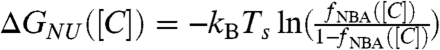. The linear fit (Fig. 1C), ΔG_NU([C]) = ΔG_NU([0]) + m[C], yields ΔG_NU([0]) = -3.4 kcal/mol and m = 1.34 kcal/mol·M. We also computed ΔG_NU([C]) using free energy profiles as a function of χ (Eq. S16), and obtained m = 1.47 kcal/mol·M. The experimentally inferred m value using circular dichroism is 1.5 kcal/mol·M whereas m = 1.6 kcal/mol·M using fluorescence measurements. The values from our simulation for m (1.34–1.47) kcal/mol·M are in excellent agreement with experimental estimates, which further shows that MTM can predict the global thermodynamic properties accurately.

Although the calculated value of ΔG_NU([0]) is in good agreement with the experimental result, it is not as accurate as m-value because of the known difficulties in obtaining accurate results at low GdmCl concentrations (40). To ensure that MTM can predict ΔG_NU([0]) accurately we calculated f_NBA([C]) for urea (green squares in Fig. 1B) from which we obtained ΔG_NU([C]) (Fig. 1C). The linear fit yields ΔG_NU([0]) = -4.2 kcal/mol, which is in excellent agreement with measurements. The m value for urea is 0.92 kcal/mol·M (less than m for GdmCl), which is consistent with the observation that folding is less cooperative in urea than in GdmCl (Fig. 1B). The results also confirm that GdmCl is more efficient (C_m = 2.5 M) in unfolding proteins than urea (C_m = 4.7 M). Our predictions for equilibrium folding in urea can be experimentally tested.

Equilibrium Collapse.

The dependence of , where r_ij is the distance between all interaction centers of the protein and N (= 112 for src SH₃) is the total number of beads, on [C] shows compaction of the denatured state ensemble (DSE) structures of SH₃ domain below C_m (Fig. 2A). By following the population of conformations in the unfolded basin of attraction (UBA) and native basin of attraction (NBA) separately, (see Fig. S1 for description of UBA and NBA using χ as the order parameter) we find that R_g of the NBA () is nearly independent of [C] (Fig. 2A). In contrast, the size of the structures in the UBA decrease continuously (41) and is about 17% more compact under folding condition than at high [C]( > C_m) (Fig. 2A). The variations in the size of the UBA, , as [C] is decreased, is reflected in the [C]-dependent changes in 〈R_g〉 (black circles in Fig. 2A). If the collapse of the DSE is neglected then , the value at [C] = 8.0 M (Fig. 2A). The distribution P(R_g) of R_g shows that as [C] increases src SH₃ samples extended conformations with R_g exceeding 30 Å (Fig. 2B). Comparison of P(R_g) of the DSE below C_m (Fig. 2A, Inset) and above C_m (the DSE region at high [C] in Fig. 2B, Inset) shows that compact conformations (R_g < 15 Å) in DSE are sampled only under folding conditions. Compaction of DSE below C_m implies that the dynamics of unfolded states must be different under folding conditions relative to high [C] as shown recently for protein L (42).

Fig. 2.

Equilibrium collapse. (A) Average 〈R_g〉 (black circles) as a function of GdmCl concentration. Red and green corresponds to 〈R_g〉 for folded and unfoled structures, respectively. Blue symbol is constructed using 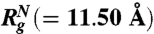, at [C] = 8.0 M, and f_NBA([C]) (see text for details). The Inset shows P(R_g) at [C] = 1.0 M for DSE. (B) Distribution P(R_g) of radius of gyration R_g for various concentrations of GdmCl. The Inset shows P(R_g) for [C] = 0 M (black), [C] = 2.5 M (navy), and [C] = 5.0 M (orange) corresponding to the extended conformations (R_g > 15 Å).

Folding Kinetics and the Chevron Plot.

We calculated the [C]-dependent folding (unfolding) rates from folding (unfolding) trajectories, which were generated from Brownian dynamics using the effective energy function, H_P({r_i},[C]) (Eq. 3 and SI Text for details). From sixty (fifty for [C] = 0) folding trajectories the fraction of unfolded molecules at time t, is computed using 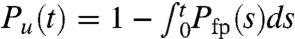, where P_fp(s) is the distribution of first passage times. For some of the [C] values, we fit P_u(t) ≈ e^-tk_f[C] under folding conditions ([C] < C_m) from which k_f([C]) can be extracted. Similarly, a single exponential fit for some values of [C] > C_m yields k_u([C]). At high (low) [C], we can approximate k_obs = k_f([C]) + k_u([C]) as k_u([C]) (k_f([C])). For [C] = 2.5 M and 3.0 M (≈C_m) the folding and unfolding rates are comparable, k_u([C]) ≈ k_f([C]). At these concentrations we performed both folding and unfolding simulations and by fitting the results for P_u(t) using exponential function we extracted k_u([C]) and k_f([C]) (see SI Text for details). We obtained k_u([0]) by globally fitting the relaxation rate, k_obs = k_f([C]) + k_u([C]), using ln k_obs = ln[k_f([0])e^-m_f[C]/RT + k_u([0])e^m_u[C]/RT], where m_f (m_u) is the slope of the folding (unfolding) arm with ln k_f = ln k_f(0) - m_f[C]/RT and ln k_u = ln k_u(0) + m_u[C]/RT.

The dependence of P_u(t) at [C] = 0.0 M, 1.0 M, and 5.0 M as a function of t is given in Fig. 3A. For [C] = 5.0 M, P_u(t) represents the fraction of conformations in the NBA. Clearly, k_f([C]) decreases as [C] increases, and k_u([C]) increases as [C] increases. Most importantly, plot of ln k_obs as a function of [C] over the concentration range (0 M ≤ [C] ≤ 6.5 M) of GdmCl shows a classic chevron shape (Fig. 3B). For [C] = 0 ∼ 2.0 M, k_u ≪ k_f, so that k_obs ≈ k_f and similarly for [C] above 3.5 M, k_obs ≈ k_u. In the transition region, k_f ≈ k_u, which requires generation of a large number of trajectories, k_obs([C]) converges slowly resulting in larger errors. Comparison of the simulation and experimental results (filled black circles in Fig. 3B) allows us to draw two major conclusions. (i) The slopes (from the folding and unfolding arms) of the simulated chevron plot are surprisingly similar to the experimental values. (ii) Within error bars in simulations and experiments, we do not find any deviation from linearity in the chevron plot. Taken together, our simulation results for k_obs[C] semiquantitatively capture all of the experimental features, which is remarkable given the simplicity of the MTM.

Fig. 3.

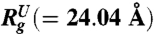
Folding kinetics. (A) Fraction of molecules that have not folded ([C] = 0.0 M, and [C] = 1.0 M) or unfolded ([C] = 5.0 M) as a function of time. The lines are exponential fits to the data. (B) Comparison of chevron plots obtained from simulations and experiment. The scale for the experimental plot for is on the left, and for the simulations is on the right. The slopes of the calculated folding (m_f) and unfolding (m_u) are 0.95 kcal/mol·M and 0.60 kcal/mol·M, respectively, which are in good agreement with experiment.

Consistency Between Thermodynamics and Kinetics.

From the slope of the folding arm (simulation results in Fig. 3B), we obtain m_f = 0.95 kcal/mol·M and m_u = 0.60 kcal/mol·M from the unfolding arm. The corresponding experimental values are 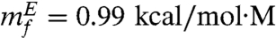and 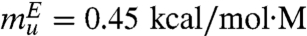, which shows very good agreement between experiments and simulations although m_u is somewhat higher than . For a two-state description, thermodynamics and kinetics simulations should be consistent, and hence we expect m ≈ m_f + m_u. From the simulated chevron plot, we obtain m ≈ 1.55 kcal/mol·M, which is in excellent agreement with m (1.34–1.47 kcal/mol·M) obtained from equilibrium calculations (Fig. 1C). The midpoint C_m at which k_f ≈ k_u is C_m ≈ 2.2 M (Fig. 3B), which nearly coincides with C_m = 2.5 M calculated using f_NBA[C_m] = 0.5 (Fig. 1B). Thus, both thermodynamic and kinetic results obtained using MTM simulations are in harmony, and justifies the two-state description for src SH₃ folding.

Comparison of simulation and experiments shows that although MTM simulations reproduce the chevron shape well, the dependence of ln k_obs on [C] does not quantitatively agree with experiments. In particular, k_f([0]) from simulations is 925.9 s^-1 whereas the extrapolated value to [C] = 0 from experiment is 56.7 s^-1. Thus, the folding rate from MTM simulations is about 16 times faster that the experimental rate. Deviations from experiments increase to about 40 at C ∼ C_m. The differences between k_u([C]) obtained using simulations and experiments are larger. For example, k_u([C] = 5.0 M) differs by a factor of approximately 150 from experiments (Fig. 3B). The unfolding rate k_u([0]) (the value in water) from our simulations is k_u([0]) ≈ 7.60 s^-1, whereas the extrapolated rate from experiment is 0.1 s^-1. The larger discrepancy in k_u([0]) between simulations and experiments is due to the substantial error in the simulations, which occurs because relatively small number of unfolding events are observed at low [C]. The agreement with experiments could be improved further by taking into account the changes in the denaturant-dependent changes in viscosity. Nevertheless, from the calculated k_f([0]) and k_u([0]) values, we infer that , which compares favorably with estimates from thermodynamic simulations. The coincidence of m value calculated from the linear dependence of ΔG_NU([C]) with m_f + m_u obtained from chevron plot, and the similarity between ΔG_NU([0]) and the estimate using k_f([0]) and k_u([0]) allows us to conclude that a two-state model is accurate for folding of src SH₃. Although such a conclusion has been reached using experiments it is gratifying that we can capture the global aspects of folding thermodynamics and kinetics using simulations based on MTM.

Collapse Kinetics, Folding, and Unfolding Pathways.

The kinetics of collapse of src SH₃ domain at [C] = 0 and [C] = 1.0 M shows (Fig. 4A) that 〈R_g(t)〉 decays with a single rate constant, k_c([C]), the rate of collapse. The values of k_c([C]) from the data in Fig. 4A are similar to k_f([C]), which shows compaction and folding occur nearly simultaneously. The inset shows P(R_g; t) at t = 0, t ≈ τ_c ≈ (k_c([C] = 1.0 M))^-1 ≈ 4.2 ms, and t = 34 ms (the first passage time for the slowest trajectory), respectively. Even after collapse (t ≈ τ_c) the protein samples, with small probability (middle inset), conformations with R_g > 12 Å (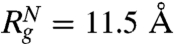). Thus, the ensemble of kinetically collapsed conformations is a mixture of folded and specific (native-like) and nonspecific compact structures (43). Although at an ensemble level k_c([C]) ≈ k_f([C]), examination of the dynamics of acquisition of structure (χ(t) as a function of t in Fig. S2) shows heterogeneity, which is masked in the ensemble averages. The link between compaction and acquisition of secondary structure, measured in terms of fraction (f_ss) of secondary structure element, shows that these two processes also occur simultaneously (Fig. 4B) in src SH₃. Due to the cooperative nature of folding there is very little dependence of these processes on [C].

Fig. 4.

Folding and unfolding pathways. (A) Collapse kinetics monitored by the time-dependent average 〈R_g(t)〉 as a function of t. Collapse (expansion) decreases (increases) in 〈R_g(t)〉 can be fit using a single exponential function. The Inset shows P(R_g; t) at t = 0, t ≈ τ_c ≈ (k_c([C] = 1.0 M))^-1 ≈ 4.2 ms, and t = 34 ms, the first passage time for the slowest trajectory, respectively. (B) Projection of kinetic folding trajectories in terms of fraction of secondary structure formation, f_ss, and 〈R_g〉. (C) First passage time for formation of various interactions, indicated in the figure, from the sixty folding trajectories at [C] = 1.0 M. The solid black symbols show the correlation between and , which are first passage times for formation of interactions β₁ - β₂ and β₂ - β₃, respectively. (D) Same as (C) except the results are for unfolding at [C] = 6.0 M. Similarity between (C) and (D) establishes the reversibility between folding and unfolding.

Kinetic cooperativity is most vividly illustrated in Fig. 4C for [C] = 1.0 M and Fig. 4D for [C] = 6.0 M. In Fig. 4c, we plot the first passage times for reaching the native state at [C] = 1.0 M and for establishment of interactions involving various structural elements for the sixty folding trajectories. All the first passage times coincide (all measures of structure content form at the same time), which shows that in the final stages (after crossing the free energy barrier) the entire structure is consolidated simultaneously. Similarly, unfolding at [C] = 6.0 M as measured by loss of structures of the whole protein or various fragments (β₁₂, β₂₃, β₃₄, and β₄₅) also occur simultaneously (Fig. 4D). The black symbols in Fig. 4 C and D shows the correlation between the first passage times for establishing interactions between β1 - β2 and β2 - β3. The quantitative picture that emerges is that unfolding and folding in src SH₃ occurs in a single step in a highly cooperative manner although there is pathway diversity in the dynamics of individual folding trajectories (Fig. S2).

Structures of the Transition State Ensemble (TSE).

We first determined P(δ), the probability of forming native contacts as a function of the progress variable δ = t/τ_1i, where τ_1i is the first passage time for the ith trajectory. The values of δ_TS where dP/dδ starts to increase rapidly is identified with the transition state (TS) region, and the conformations in this neighborhood are grouped to obtain the TSE (44). We determined the structures of the TSE using a procedure that is similar to the progress variable clustering method (45, 46), which uses a neural network algorithm to classify TSE structures without using surrogate reaction coordinates.

The global characteristics of the TSE is experimentally described using the Tanford β_f = m_f/m (or β_u = 1 - β_f). From the experimental chevron plot 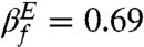whereas our simulations give . It is generally assumed that β_f is related to the buried solvent accessible surface area (SASA) at the TS. For the TSE obtained in our simulations, we calculated the [C]-dependent distribution P(Δ_R) (see Fig. 5A for [C] = 1.0 M), where Δ_R = (Δ_U - Δ_TSE)/(Δ_U - Δ_N) and Δ_U, Δ_TSE, Δ_N are the SASA values in the DSE ([C] = 6.0 M), TSE, and the NBA ([C] = 1.0 M), respectively. We found that the average 〈Δ_R〉 = 0.68. The close correspondence between (or ) and 〈Δ_R〉 affirms the standard interpretation of the Tanford parameter. The small fluctuation, , shows that the TSE in src SH₃ is conformationally restricted.

Fig. 5.

Transition state ensemble structures. (A) Distribution P(Δ_R), of the Δ_R = (Δ_U - Δ_TSE)/(Δ_U - Δ_N), which is the fraction of buried solvent accessible surface area relative to the unfoled structures. The average values of Δ_N and Δ_U are 5270 Å² and 8189 Å², respectively. The average 〈Δ_R〉 = 0.68, which coincides with Tanford β parameter. (B) Contact map of the native state ensemble (Upper Left) and the one for the TSE structures (Lower Right). The scale on the right gives the probablity of contact formation. The number of native contacts in the folded state is 507. (C) Superposition of a few structures of the dominant TSE cluster (Left) shows formation of the core with disorder mostly in the RT loop (see text). The subdominant cluster has well-formed β₁, β₂, and β₃ hydrophobic core.

From the lower half of Fig. 5B, which shows the contact map obtained from the TSE structures, it is clear that relative to the native state (top half) there are variations in the extent to which the structure is ordered in the transition region. The core of the protein involving interactions in strands β₁, β₂ and to a lesser extent β₃ form with substantial probability in the TSE. The distal loop is structured in the TS as are residues involving the diverging turn. It is likely that the necessity to form the distal loop due to its intrinsic stiffness forces the core of the protein to be ordered in the TSE (37, 47). Residues from the n-src loop that are part of the hydrophobic core form with great probability in the TSE. However, the RT-loop, with large conformational fluctuations in the transition state, is disordered in the TSE (structures on the left in Fig. 5C).

We classified the TSE structures according to the similarity to the native state for [C] = 1.0 M (Fig. 5C). In the dominant transition state (found in approximately 72% of the folding trajectories) the core of the structures comprised of β₁, β₂, and β₃ is packed orthogonally as in the native state (structures in Fig. 5C, Left). The subdominant member of the TSE (approximately 12%) also has a well-formed central β-sheet but are otherwise not well structured (conformation of Fig. 5C, Right). The calculated average structure of the dominant TSE conformations is similar to that inferred from experimental ϕ-value analysis. The common features of the TSE is that the central β₁, β₂, β₃ strands are well structured as are residues in the distal loop. The present and previous simulations using entirely different models and methods of determining the TSE structures, are also in very good agreement (36, 38). Both the structures, which are consistent with experiments, show that contacts involving β₁ - β₂ sheet and the RT loop forms with low probability. Although simulations predict a single dominant transition state structure, diversity (assessed by probability distribution of contact formation or P(Δ_R)) in the TSE structures, which is hard to glean from experiments, points to the inherent plasticity of the TSE, even in SH₃ domains in which there is predominantly a single transition state.

Discussion

Collapse Transition.

Based on Flory theory we expect that radius of gyration must scale as (ν ≈ 0.6, a_D ≈ 2 Å)(48) at high [C]. Similarly, in the folded state (49). The predicted theoretical values ( and ) are in very good agreement with simulation results. Using the values for (≈24.04 Å at [C] = 8.0 M in Fig. 2A) and (≈11.50 Å) a theoretical estimate can be made. However, Fig. 2A shows that does not agree with 〈R_g〉. Because the changes in 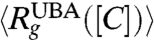in small single domain proteins are not large (20–30%), which predominantly occur below C_m where the population of molecules in the UBA is small, it is in general difficult to detect them using standard small angle X-ray scattering (SAXS) methods. However, a recent study using SAXS has reported continuous reduction in as [C] is lowered in dihydrofolate reductase (50), a protein with approximately 150 amino acid residues. Single molecule experiments also show unambiguous features of collapse for protein L and cold shock protein.

In the folding of src SH₃ protein, collapse process and acquisition of native structure occur nearly simultaneously (Fig. 4). On the time scale of collapse we find that only about 50% of the secondary structures are fully formed (Fig. 4B), which implies that there is a dynamic coexistence between folded and unfolded states. In contrast, in the folding of Cytochrome c, monitored by SAXS and CD, it has been shown that collapse is preceded by acquisition of secondary structure (51, 52). We suggest that with decreased cooperativity there could be a separation in the time scale between these two distinct processes (53).

Folding Kinetics.

The most important achievement of our study is the simulation of the chevron plot. The difference between the calculated and measured k_obs could arise from neglect of nonnative interactions and possibly from not using explicit models for water and GdmCl. Although one can appeal to extensive studies using lattice and offlattice models (44), which show that to a large extent the folding mechanisms for foldable sequences are not greatly altered by including nonnative interactions, their role has to be quantitatively assessed. Nonnative interactions are likely not relevant either at very high or very low [C] values but do play an important role in affecting the thermodynamics in the transition region (Fig. 1B). Despite these reservations the remarkable agreement between simulations and experiments shows that the theory outlined here can yield fundamental insights into protein folding using higher resolution models.

Concluding Remarks

We have produced the most comprehensive picture of denaturant-dependent folding of src SH₃ domain using simulations that include denaturant effects in conjunction with self-organized polymer-side chain (SOP-SC) model for the polypeptide chain. Results for folding thermodynamics are in quantitative agreement with experiments. Somewhat surprisingly it is found that not only do the calculations reproduce the chevron plot but the predicted values of the [C]-dependent folding rates are in reasonable agreement with measurements. The nearly [C]-independent structure of the dominant transition state structure is broadly consistent with the structural interpretation based on Φ-value analysis and simulations (at [C] = 0) carried out using entirely different model and methods. Our work shows that the Tanford β-parameter measures the fraction of buried SASA in the TSE. The theory underlying the MTM is general and can be adopted in conjunction with all-atom representation of proteins, thus making it feasible to study denaturant and osmolyte effects using simulations.

Methods

SOP-Sidechain Model.

Simulations were carried out using the SOP model (54) each residue is represented by two interaction centers, one that is located at the C_α position and the other is at the center of mass of the side chain. Native state is stabilized by backbone–backbone, side chain–side chain, and backbone–side chain interactions. For the side chain–side chain interactions we use the Betancourt–Thirumalai statistical potential (55). The effective energy, obtained by integrating over solvent (water) degrees of freedom, which describes the intrapeptide interactions of the polypeptide chain with coordinates {r_i}, is

[1]

Detailed descriptions of the terms in Eq. 1 and the parameters of the forcefield are in Tables S1 and S2. We use low friction Langevin simulations to obtain thermodynamic properties (56). Folding trajectories are generated using a Brownian dynamics algorithm (57) using a friction coefficient that corresponds to water viscosity (see SI Text for details).

Molecular Transfer Model.

The free energy of transferring a protein conformation described by {r_i} from water ([C] = 0) to aqueous denaturant solution ([C] ≠ 0) is approximated (58, 59) as

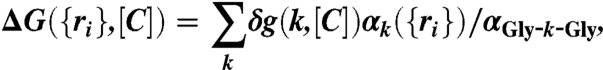[2]

where the sum is over backbone and side chain, δg(k,[C]) = m_k[C] + b_k (see Table S3 for m_k and b_k values, and Table S4 for α_Gly-k-Gly values) is the transfer free energy of group k (60, 61), α_k({r_i}) is the SASA of k, and α_Gly-k-Gly is the SASA of the kth group in the tripeptide Gly-k-Gly. Thus, the effective free energy function for a protein at [C] ≠ 0 is

[3]

We used the procedure in (29), which is accurate provided exhaustive sampling using E_P({r_i}) is performed, to obtain thermodynamic properties. We use the full effective free energy function (Eq. 3) to generate folding and unfolding trajectories at [C] ≠ 0 (see SI Text for details). We compute α_k({r_i}) and using the procedure in ref. 62. Note that MTM does not assume whether the protein folds by a two-state or multistate mechanism. If E_P({r_i}) captures the nature of folding the MTM can accurately describe the effect of denaturants.

References

- 1.Schuler B, Eaton WA. Protein folding studied by single-molecule FRET. Curr Opin Struct Biol. 2008;18:16–26. doi: 10.1016/j.sbi.2007.12.003. [DOI] [PMC free article] [PubMed] [Google Scholar]
- 2.Nickson AA, Clarke J. What lessons can be learned from studying the folding of homologous proteins? Methods. 2010;52:38–50. doi: 10.1016/j.ymeth.2010.06.003. [DOI] [PMC free article] [PubMed] [Google Scholar]
- 3.Borgia A, Williams PM, Clarke J. Single-molecule studies of protein folding. Annu Rev Biochem. 2008;77:101–125. doi: 10.1146/annurev.biochem.77.060706.093102. [DOI] [PubMed] [Google Scholar]
- 4.Bartlett AI, Radford SE. An expanding arsenal of experimental methods yields an explosion of insights into protein folding mechanisms. Nat Struct Mol Biol. 2009;16:582–588. doi: 10.1038/nsmb.1592. [DOI] [PubMed] [Google Scholar]
- 5.Shank EA, Cecconi C, Dill JW, Marqusee S, Bustamante C. The folding cooperativity of a protein is controlled by its chain topology. Nature. 2010;465:637–640. doi: 10.1038/nature09021. [DOI] [PMC free article] [PubMed] [Google Scholar]
- 6.Gebhardt JCM, Bornschloegla T, Rief M. Full distance-resolved folding energy landscape of one single protein molecule. Proc Natl Acad Sci USA. 2010;107:2013–2018. doi: 10.1073/pnas.0909854107. [DOI] [PMC free article] [PubMed] [Google Scholar]
- 7.Onuchic JN, Wolynes PG. Theory of protein folding. Curr Opin Struct Biol. 2004;14:70–75. doi: 10.1016/j.sbi.2004.01.009. [DOI] [PubMed] [Google Scholar]
- 8.Thirumalai D, Hyeon C. RNA and protein folding: Common themes and variations. Biochemistry. 2005;44:4957–4970. doi: 10.1021/bi047314+. [DOI] [PubMed] [Google Scholar]
- 9.Shakhnovich E. Protein folding thermodynamics and dynamics: Where physics, chemistry, and biology meet. Chem Rev. 2006;106:1559–1588. doi: 10.1021/cr040425u. [DOI] [PMC free article] [PubMed] [Google Scholar]
- 10.Dill KA, Ozkan BS, Shell M, Weikl TR. The protein folding problem. Ann Rev Biophys. 2008;37:289–316. doi: 10.1146/annurev.biophys.37.092707.153558. [DOI] [PMC free article] [PubMed] [Google Scholar]
- 11.Munoz V, Eaton W. A simple model for calculating the kinetics of protein folding from three-dimensional structures. Proc Natl Acad Sci USA. 1999;96:11311–11316. doi: 10.1073/pnas.96.20.11311. [DOI] [PMC free article] [PubMed] [Google Scholar]
- 12.Kubelka J, Henry E, Cellmer T, Hofrichter J, Eaton W. Chemical, physical, and theoretical kinetics of an ultrafast folding protein. Proc Natl Acad Sci USA. 2008;105:18655–18662. doi: 10.1073/pnas.0808600105. [DOI] [PMC free article] [PubMed] [Google Scholar]
- 13.Thirumalai D, O’Brien EP, Morrison G, Hyeon C. Theoretical perspectives on protein folding. Ann Rev Biophys. 2010;39:159–183. doi: 10.1146/annurev-biophys-051309-103835. [DOI] [PubMed] [Google Scholar]
- 14.Pincus DL, Cho S, Hyeon C, Thirumalai D. Progress in Molecular Biology and Translational Science. Vol. 84. London: Academic; 2008. Minimal models for proteins and RNA: From folding to function; pp. 203–250. [DOI] [PubMed] [Google Scholar]
- 15.Whitford PC, et al. An all-atom structure-based potential for proteins: Bridging minimal models with all-atom empirical forcefields. Proteins. 2009;75:430–441. doi: 10.1002/prot.22253. [DOI] [PMC free article] [PubMed] [Google Scholar]
- 16.Zhang Z, Chan HS. Competition between native topology and nonnative interactions in simple and complex folding kinetics of natural and designed proteins. Proc Natl Acad Sci USA. 2010;107:2920–2925. doi: 10.1073/pnas.0911844107. [DOI] [PMC free article] [PubMed] [Google Scholar]
- 17.Ziv G, Thirumalai D, Haran G. Collapse transition in proteins. Phys Chem Chem Phys. 2009;11:83–93. doi: 10.1039/b813961j. [DOI] [PMC free article] [PubMed] [Google Scholar]
- 18.Nettels D, Gopich IV, Hoffmann A, Schuler B. Ultrafast dynamics of protein collapse from single-molecule photon statistics. Proc Natl Acad Sci USA. 2007;104:2655–2660. doi: 10.1073/pnas.0611093104. [DOI] [PMC free article] [PubMed] [Google Scholar]
- 19.Sherman E, Haran G. Coil-globule transition in the denatured state of a small protein. Proc Natl Acad Sci USA. 2006;103:11539–11543. doi: 10.1073/pnas.0601395103. [DOI] [PMC free article] [PubMed] [Google Scholar]
- 20.Merchant KA, Best RB, Louis JM, Gopich IV, Eaton WA. Characterizing the unfolded states of proteins using single-molecule FRET spectroscopy and molecular simulations. Proc Natl Acad Sci USA. 2007;104:1528–1533. doi: 10.1073/pnas.0607097104. [DOI] [PMC free article] [PubMed] [Google Scholar]
- 21.Sadqi M, Lapidus LJ, Munoz V. How fast is protein hydrophobic collapse? Proc Natl Acad Sci USA. 2003;100:12117–12122. doi: 10.1073/pnas.2033863100. [DOI] [PMC free article] [PubMed] [Google Scholar]
- 22.Chung HS, Louis JM, Eaton WA. Experimental determination of upper bound for transition path times in protein folding from single-molecule photon-by-photon trajectories. Proc Natl Acad Sci USA. 2009;106:11837–11844. doi: 10.1073/pnas.0901178106. [DOI] [PMC free article] [PubMed] [Google Scholar]
- 23.Jackson S. How do small single-domain proteins fold? Fold Des. 1998;3:R81–R91. doi: 10.1016/S1359-0278(98)00033-9. [DOI] [PubMed] [Google Scholar]
- 24.Clementi C. Coarse-grained models of protein folding: Toy models or predictive tools? Curr Opin Struct Biol. 2007;17:1–6. doi: 10.1016/j.sbi.2007.10.005. [DOI] [PubMed] [Google Scholar]
- 25.Karanicolas J, Brooks CL., III The origins of asymmetry in the folding transition states of protein L and protein G. Protein Sci. 2002;11:2351–2361. doi: 10.1110/ps.0205402. [DOI] [PMC free article] [PubMed] [Google Scholar]
- 26.Oliveberg M, Wolynes PG. The experimental survey of protein-folding energy landscapes. Q Rev Biophys. 2005;38:245–288. doi: 10.1017/S0033583506004185. [DOI] [PubMed] [Google Scholar]
- 27.Clementi C, Nymeyer H, Onuchic J. Topological and energetic factors: What determines the structural details of the transition state ensemble and “en-route” intermediates for protein folding? An investigation for small globular proteins. J Mol Biol. 2000;298:937–953. doi: 10.1006/jmbi.2000.3693. [DOI] [PubMed] [Google Scholar]
- 28.Fernandez-Escamilla AM, et al. Solvation in protein folding analysis: Combination of theoretical and experimental approaches. Proc Natl Acad Sci USA. 2004;101:2834–2839. doi: 10.1073/pnas.0304180101. [DOI] [PMC free article] [PubMed] [Google Scholar]
- 29.O’Brien EP, Ziv G, Haran G, Brooks BR, Thirumalai D. Effects of denaturants and osmolytes on proteins are accurately predicted by the molecular transfer model. Proc Natl Acad Sci USA. 2008;105:13403–13408. doi: 10.1073/pnas.0802113105. [DOI] [PMC free article] [PubMed] [Google Scholar]
- 30.O’Brien EP, Brooks BR, Thirumalai D. Molecular origin of constant m-values, denatured state collapse, and residue-dependent transition midpoints in globular proteins. Biochemistry. 2009;48:3743–3754. doi: 10.1021/bi8021119. [DOI] [PMC free article] [PubMed] [Google Scholar]
- 31.O’Brien EP, Morrison G, Brooks BR, Thirumalai D. How accurate are polymer models in the analysis of Forster resonance energy transfer experiments on proteins? J Chem Phys. 2009;130:124903. doi: 10.1063/1.3082151. [DOI] [PMC free article] [PubMed] [Google Scholar]
- 32.Riddle DS, et al. Experiment and theory highlight role of native state topology in SH3 folding. Nat Struct Biol. 1999;6:1016–1024. doi: 10.1038/14901. [DOI] [PubMed] [Google Scholar]
- 33.Grantcharova VP, Riddle DS, Baker D. Long-range order in the src SH3 folding transition state. Proc Natl Acad Sci USA. 2000;97:7084–7089. doi: 10.1073/pnas.97.13.7084. [DOI] [PMC free article] [PubMed] [Google Scholar]
- 34.Grantcharova VP, Baker D. Folding dynamics of the src SH3 domain. Biochemistry. 1997;36:15685–15692. doi: 10.1021/bi971786p. [DOI] [PubMed] [Google Scholar]
- 35.Martinez J, Serrano L. The folding transition state between SH3 domains is conformationally restricted and evolutionarily conserved. Nat Struct Biol. 1999;6:1010–1016. doi: 10.1038/14896. [DOI] [PubMed] [Google Scholar]
- 36.Hubner IA, Edmonds KA, Shakhnovich EI. Nucleation and the transition state of the SH3 domain. J Mol Biol. 2005;349:424–434. doi: 10.1016/j.jmb.2005.03.050. [DOI] [PubMed] [Google Scholar]
- 37.Klimov D, Thirumalai D. Stiffness of the distal loop restricts the structural heterogeneity of the transition state ensemble in SH3 domains. J Mol Biol. 2002;317:721–737. doi: 10.1006/jmbi.2002.5453. [DOI] [PubMed] [Google Scholar]
- 38.Ding F, Guo WH, Dokholyan NV, Shakhnovich EI, Shea JE. Reconstruction of the src-SH3 protein domain transition state ensemble using multiscale molecular dynamics simulations. J Mol Biol. 2005;350:1035–1050. doi: 10.1016/j.jmb.2005.05.017. [DOI] [PubMed] [Google Scholar]
- 39.Klimov D, Thirumalai D. Cooperativity in protein folding: From lattice models with side chains to real proteins. Fold Des. 1998;3:127–139. doi: 10.1016/s1359-0278(98)00018-2. [DOI] [PubMed] [Google Scholar]
- 40.Makhatadze G. Thermodynamics of protein interactions with urea and guanidinium hydrochloride. J Phys Chem B. 1999;103:4781–4785. [Google Scholar]
- 41.Dasgupta A, Udgaonkar J. Evidence for initial non-specific polypeptide chain collapse during the refolding of the SH3 domain of PI3 kinase. J Mol Biol. 2010;403:430–445. doi: 10.1016/j.jmb.2010.08.046. [DOI] [PubMed] [Google Scholar]
- 42.Waldauer S, Bakajin O, Lapidus L. Extremely slow intramolecular diffusion in unfolded protein L. Proc Natl Acad Sci USA. 2010;107:13713–13717. doi: 10.1073/pnas.1005415107. [DOI] [PMC free article] [PubMed] [Google Scholar]
- 43.Camacho CJ, Thirumalai D. Minimum energy compact structures of random sequences of heteropolymers. Phys Rev Lett. 1993;71:2505–2508. doi: 10.1103/PhysRevLett.71.2505. [DOI] [PubMed] [Google Scholar]
- 44.Klimov D, Thirumalai D. Multiple protein folding nuclei and the transition state ensemble in two state proteins. Proteins. 2001;43:465–475. doi: 10.1002/prot.1058. [DOI] [PubMed] [Google Scholar]
- 45.Guo Z, Thirumalai D. The nucleation-collapse mechanism in protein folding: Evidence for the non-uniqueness of the folding nucleus. Fold Des. 1997;2:377–391. doi: 10.1016/S1359-0278(97)00052-7. [DOI] [PubMed] [Google Scholar]
- 46.Klimov D, Thirumalai D. Lattice models for proteins reveal multiple folding nuclei for nucleation-collapse mechanism. J Mol Biol. 1998;282:471–492. doi: 10.1006/jmbi.1998.1997. [DOI] [PubMed] [Google Scholar]
- 47.Spagnolo L, Ventura S, Serrano L. Folding specificity induced by loop stiffness. Protein Sci. 2003;12:1473–1482. doi: 10.1110/ps.0302603. [DOI] [PMC free article] [PubMed] [Google Scholar]
- 48.Kohn J, et al. Random-coil behavior and the dimensions of chemically unfolded proteins. Proc Natl Acad Sci USA. 2004;101:12491–12496. doi: 10.1073/pnas.0403643101. [DOI] [PMC free article] [PubMed] [Google Scholar]
- 49.Dima R, Thirumalai D. Asymmetry in the shapes of folded and denatured states of proteins. J Phys Chem B. 2004;108:6564–6570. [Google Scholar]
- 50.Arai M, et al. Microsecond hydrophobic collapse in the folding of Escherichia coli Dihydrofolate reductase, an alpha/beta-type protein. J Mol Biol. 2007;368:219–229. doi: 10.1016/j.jmb.2007.01.085. [DOI] [PubMed] [Google Scholar]
- 51.Akiyama S, et al. Conformational landscape of cytochrome C folding studied by microsecond-resolved small-angle X-ray scattering. Proc Natl Acad Sci USA. 2002;99:1329–1334. doi: 10.1073/pnas.012458999. [DOI] [PMC free article] [PubMed] [Google Scholar]
- 52.Cardenas A, Elber R. Kinetics of cytochrome C folding: Atomically detailed simulations. Proteins. 2003;51:245–257. doi: 10.1002/prot.10349. [DOI] [PubMed] [Google Scholar]
- 53.Thirumalai D. From minimal models to proteins: Time scales for protein folding kinetics. J Phys I. 1995;5:1457–1467. [Google Scholar]
- 54.Hyeon C, Dima RI, Thirumalai D. Pathways and kinetic barriers in mechanical unfolding and refolding of RNA and proteins. Structure. 2006;14:1633–1645. doi: 10.1016/j.str.2006.09.002. [DOI] [PubMed] [Google Scholar]
- 55.Betancourt M, Thirumalai D. Pair potentials for protein folding: Choice of reference states and sensitivity of predicted native states to variations in the interaction schemes. Protein Sci. 1999;8:361–369. doi: 10.1110/ps.8.2.361. [DOI] [PMC free article] [PubMed] [Google Scholar]
- 56.Guo Z, Thirumalai D. Kinetics and thermodynamics of folding of a de novo designed four helix bundle. J Mol Biol. 1996;263:323–343. doi: 10.1006/jmbi.1996.0578. [DOI] [PubMed] [Google Scholar]
- 57.Ermak D, McCammon J. Brownian dynamics with hydrodynamic interactions. J Chem Phys. 1978;69:1352–1360. [Google Scholar]
- 58.Pace C. Determination and analysis of urea and guanidine hydrochloride denaturation curves. Methods Enzymol. 1986;131:266–280. doi: 10.1016/0076-6879(86)31045-0. [DOI] [PubMed] [Google Scholar]
- 59.Nozaki Y, Tanford C. Solubility of amino acids and related compounds in aqueous urea solutions. J Am Chem Soc. 1963;288:4074–4081. [PubMed] [Google Scholar]
- 60.Auton M, Bolen D. Additive transfer free energies of the peptide backbone unit that are independent of the model compound and the choice of concentration scale. Biochemistry. 2004;43:1329–1342. doi: 10.1021/bi035908r. [DOI] [PubMed] [Google Scholar]
- 61.Auton M, Holthauzen L, Bolen D. Anatomy of energetic changes accompanying urea-induced protein denaturation. Proc Natl Acad Sci USA. 2007;104:15317–15322. doi: 10.1073/pnas.0706251104. [DOI] [PMC free article] [PubMed] [Google Scholar]
- 62.Hayryan S, Hu CK, Skrivanek J, Hayryan E, Pokorny I. A new analytical method for computing solvent-accessible surface area of macromolecules and its gradients. J Comput Chem. 2005;26:334–343. doi: 10.1002/jcc.20125. [DOI] [PubMed] [Google Scholar]
Associated Data
This section collects any data citations, data availability statements, or supplementary materials included in this article.