Abstract
Complex feedback systems are ubiquitous in biology. Modeling such systems with mass action laws or master equations requires information rarely measured directly. Thus rates and reaction topologies are often treated as adjustable parameters. Here we present a general stochastic modeling method for small chemical and biochemical systems with emphasis on feedback systems. The method, Maximum Caliber, is more parsimonious than others in constructing dynamical models requiring fewer model assumptions and parameters to capture the effects of feedback. Maximum Caliber is the dynamical analog of Maximum Entropy. It uses average rate quantities and correlations obtained from short experimental trajectories to construct dynamical models. We illustrate the method on the bistable genetic toggle switch. To test our method, we generate synthetic data from an underlying stochastic model. MaxCal reliably infers the statistics of the stochastic bistability and other full dynamical distributions of the simulated data, without having to invoke complex reaction schemes. The method should be broadly applicable to other systems.
Keywords: Stochastic dynamics, Maximum Caliber, Genetic Toggle Switch, Bistability, Feedback
Introduction
We describe a method for modeling stochastic chemical and biochemical reactions that have feedback. By feedback, we mean situations where the output of one reaction drives forwards or inhibits another reaction. Feedback is an important component of bistability, oscillations, signal amplification, noise mitigation, and biological regulation. More particularly, we focus on few-particle systems, where the raw experimental data is in the form of stochastic trajectories, and for which dynamical fluctuations can be significant. Our approach to modeling such systems aims to make minimal assumptions about the mathematical forms of the feedback mechanism, and to put maximal reliance on the experimental data itself.
Key examples of stochastic feedback in biology include the bifurcation points on fitness landscapes that account for the origins of new biological species, the mosaic patterning of the cells within the eye of the fruit fly [1, 2], bacterial evolution through a process called bet-hedging [3, 4], and many others [5, 6, 7, 8, 9, 10]. One important class of problem is stochastic bistable systems [11, 12]. These systems are driven by small fluctuations and feedback to toggle between stable states.
Often an underlying feedback mechanism is unknown or difficult to determine. In dynamical modeling, it is common to assume an arbitrary nonlinear mathematical form, for example a Hill-type model of cooperativity in a mass-action model. There are two problems with such approaches. First, often the assumed mechanism cannot be validated independently. Second, even when such a model captures the average dynamical behavior, there is no guarantee that it will accurately describe the fluctuations.
There are methods that go beyond macroscopic mass-action models to capture dynamical fluctuations to model few-particle systems. Such methods are relevant in studying the stochastically induced switches of bistable systems mentioned earlier. A principal approach involves using master equations [13] or simulations of them using Gillespie’s algorithm [14]. However, the main requirement of this approach is prior knowledge of: (1) the ‘topology’ of the reaction (i.e. a set of ‘process’ arrows interrelating ‘states’, such as substrates, products and catalysts), and (2) the values of the corresponding rate coefficients.
Many methods are thus focused on extracting rates, network topologies or other features of chemical reactions. In the method of correlated metric construction (CMC) [15, 16], time correlations in the concentrations of chemical species are used to infer the reaction topology. Species concentrations are perturbed randomly, and correlations of relaxations are monitored. The method, however, does not treat feedback, which involves more complex correlations that can arise from underlying physical time delays or memory or multistability [15]. In other cases, the aim of dynamical modeling is to assume a reaction topology and to find rates that best fit some existing experimental data trajectories[17]. For example, maximum-likelihood methods [18, 19, 20, 21] are commonly used to analyze ion-channel or fluorescence experiments [22]. There are methods to discriminate between assumed model topologies [20]. One disadvantage is that often a large number of different models will fit the same data equally well [23].
We describe a different (but related) approach called the Maximum Caliber (MaxCal) method which is the dynamical analog of Maximum Entropy[25, 24, 26, 27, 28, 29, 30, 31, 32, 33]. The MaxCal method has the advantage that the model building is data-driven and provides an unambiguous recipe for incorporating information on correlations between observable species. MaxCal bypasses the need to know the functional form or the exact details of feedback mechanism in advance, and it constructs a minimal model from the data. To illustrate the MaxCal method, we focus on an engineered cell-biological system called the genetic toggle switch [34, 35, 36, 37], which has been explored in recent experiments by Gardner et al. [34]. The toggle-switch has two very different timescales: fast time-scale fluctuations can trigger the system to switch from one state to the other, and a longer timescale over which the system remains stable in a single state. Recently Otten and Stock[32, 33] used MaxCal to infer the most likely discrete Markov model giving rise to a particular signal decay. Here our goal is different; we are interested in building an approximate model for complex systems, usually involving feedback, that will infer long time statistical properties of the system given short-time trajectories.
Methods
A Bistable Biological Circuit: the Genetic Toggle Switch
Our basic approach here is to create an underlying model of the genetic toggle switch, simulate it using Gillespie’s algorithm, and then treat those trajectories as our “data”. We use the generated data, without further inputs about the model used to generate the data, to build a MaxCal model that will make predictions regarding quantities that have not been used to parametrize it.
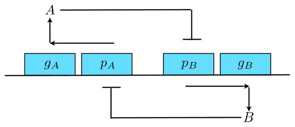
We begin by introducing the detailed model of the toggle switch we use to simulate the data. The genetic toggle switch is a bistable biological circuit whose basic topology can be described using two promoters, pA and pB, and their respective transcription products, A and B. When the gene promoter pA is activated, it produces a transcription factor, protein A, which then inhibits the promoter of a second transcription factor, protein B. Alternatively, when the promoter region pB is activated, it produces a transcription factor protein B, which then inhibits the production of protein A. The feedback network is described in Fig. (1). What follows is a proposed set of chemical reactions for a genetic toggle switch [38, 39],
Fig. 1. The genetic toggle switch.
DNA plasmid is shown with promoters pA and pB of genes gA and gB that, when transcribed, produce proteins A and B, respectively. The gene-promoter complex for species A(B) is denoted α(β) in Eq.(1). In this gene circuit, production of A inhibits B or production of B inhibits A. In Eq.(2), this is shown by having A bind to the gene-promoter complex of B, and vice-versa.
| (1) |
| (2) |
This system has three types of reaction: (1) A → φ indicates that A molecules are degraded with rate dA; similarly for B. (2) α → α + A indicates that protein A is produced at rate kα if the promoter α is active. Similarly β → β + B indicates that protein B is produced at rate kβ if the promoter β is active. (3) A + β ↔ β* indicates that protein A acts as a catalyst to convert B’s active promoter β to inactive promoter β* with rate fA. The inactivation is released with rate rA. Similarly, B + α ↔ α* indicates that protein B converts A’s active promoter α to an inactive form α* with rate fB. The inactivation is released with rate rB. Conservation requires that [α] + [α*] = 1 and [β] + [β*] = 1, where the brackets indicate concentrations of the promoters. For the exclusive toggle switch, ETS, we assume the additional constraint [α*]+[β*] ≤ 1. With the latter constraint, the only possible steady macroscopic states are (high A and low B) or (low A and high B)1.
On the one hand, the experiments on the toggle switch reveal that it is a bistable system. On the other hand, despite the fact that this is an engineered system, the physical basis for the underlying bistability in experiments is not known. At the mass action level, Gardner et al. [34] first invoked cooperative binding of transcription factors to promoters to account for the observed bistability. However, there is no independent experimental validation of that mechanism. Later stochastic modeling, based on master equations, showed that invoking binding cooperativity was unnecessary. The bistability can result from fluctuations alone [38, 39]. In this case, as in many other cases of dynamical modeling, it is not known a priori what the physical basis for complex dynamical behaviors is. Dynamical modeling is often done by first assuming a particular set of reactions (the topology) or by assuming mathematical functional forms for the rate equations (such as Michaelis-Menten or Hill terms), and then by choosing parameters for those models that best fit the experimental data. The downsides to this approach are that they provide no validation for the underlying model, because the parameters are often not obtainable independently.
We note particular advantages in using MaxCal to analyze the data generated for the ETS: (1) the MaxCal model is parametrized from the data directly, (2) the mathematical forms of the rate expressions need not be known in advance, (3) the fluctuations and higher moments of the dynamical distribution function are determined directly from the model; they provide additional information for validating the model against the experimental data, and (4) the long-time dynamical behavior can be inferred from shorter-time trajectories. In this case, the simulated data shows that there is production and disappearance of A and B and that there is an inverse correlation of populations of A with B. Without asserting a particular mechanism, i.e. reaction network topology, MaxCal uses this information to build a minimal model.
Modeling bistable systems using Maximum Caliber
The method of MaxCal is described in detail elsewhere [24, 27, 29, 30, 28, 32, 31, 33] and in the supplementary material of this paper. We summarize it briefly here. In equilibrium statistical mechanics, Jaynes showed [26] that the Boltzmann distribution law can be derived from the principle (Maximum Entropy) that all the equilibrium microstates of a system should be taken to be equivalent, except insofar as the system must satisfy some constraint on an average equilibrium quantity (in the canonical ensemble, the fixed quantity is the temperature, or equivalently, the average energy, 〈U〉). In nonequilibrium statistical mechanics, MaxCal asserts that all the trajectories (pathways) of a system should be taken as equivalent, except insofar as the system must satisfy some constraint on an average dynamical quantity, such as an average rate. In equilibrium statistical mechanics, the central quantity is a partition function, which is a weighted sum over all the accessible microstates. In MaxCal, the central quantity is a dynamical partition function, which is a weighted sum over all the possible pathways.
We briefly outline a sketch of how one computes the dynamical partition function in MaxCal and later discuss the particular case of the ETS. We begin by defining pΓ(t), or simply pΓ as the probability of observing trajectory, or pathway, Γ within some small time interval [t,t + δt] [32]. We assume that all possible trajectories within the interval [t,t + δt] are equally likely until a measurement says otherwise. Our trajectory ensemble is therefore maximally uncertain until data is used to constrain this ensemble.
In order to compute the trajectory ensemble, we maximize the caliber,
 (pΓ), which is the measure −ΣΓ pΓ ln pΓ, subject to constraints on average observables, 〈An〉,
| (3) |
where λn and α are Lagrange multipliers. In the absence of data, the first term in the above, −ΣΓ pΓ ln pΓ, simply asserts all trajectories are equally likely. Otherwise, given data, this term allows trajectories to be re-weighted in the least biased way possible according to Jaynes’ prescription[25].
Maximizing
 with respect to {pΓ}, yields
| (4) |
where Q is the dynamical analog of the equilibrium partition function. The dynamical partition function infers cumulants, subscripted c, of dynamical observables as follows
| (5) |
where m is the cumulant order.
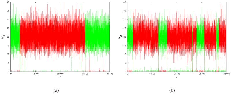
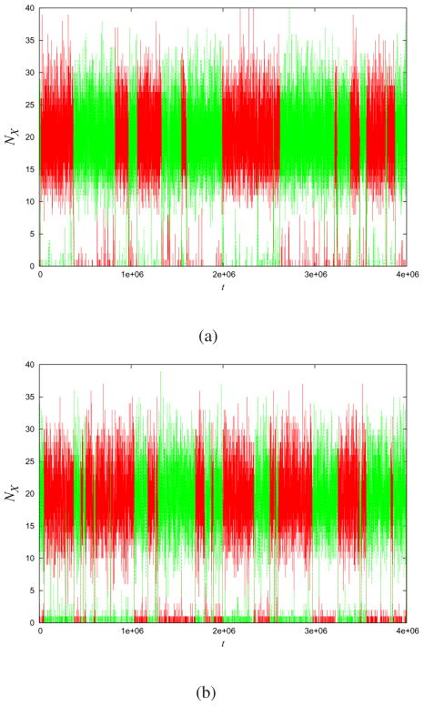
We now treat the ETS. The raw data takes the form of observed time traces of numbers of A and B molecules. The numbers of A or B molecules go up when such molecules are produced and down when such molecules are degraded. Fig. (3a) shows an example time trace. In our MaxCal treatment, we begin by subdividing the time trace into small time slices of length δt. We don’t know a priori the underlying nature of the feedback between A and B. We define two binary indicator variables for each species; one for production and one for degradation. Let ℓα be 0 when A is not produced within a small interval of length δt, or 1 otherwise. Correspondingly, ℓβ is 0 when B is not produced, and ℓβ is 1 otherwise. We choose the time interval, δt, to be sufficiently small so that no more than a single A or B is produced within it. Next, we assign variables ℓi,A and ℓi,B to each of the i individual protein molecules of type A and B, respectively. Let the variable ℓi,A or ℓi,B equal 1 when the ith particle is not degraded within interval δt or 0 otherwise.
Fig.3. Levels of promoter unbound protein A(red) and levels of unbound protein B(green).
(a) Toggle-switch trajectory generated by Gillespie model. Computer-generated trajectories using the parameters d = 0.005, k = 0.1, f = 2 and r = 0.01. The time trace was broken up into time intervals δt = 0.1. Applying MaxCal to the trajectories from (a), we extracted the Lagrange multiplier K = −0.380 and use hα = hβ = −4.605 and hA = hB = 7.6. (b) MaxCal model with parameters extracted from the simulations. Representative trajectories generated using those values in the MaxCal model.
We have introduced four types of indicator variables. We therefore require four constraints to represent the observable average protein number rise and decrease, for both types of protein, in the time trace. These observables are the production rates and degradation rates of A and B. Lagrange multipliers (hα,hA) enforce the average observed production and degradation rates of protein A while (hβ,hB) enforce the average observed production and degradation rates of protein B. For example, the statistical weight for production of a single A, say, within δt is exp(hα) (Since the time interval is chosen to be short, this statistical weight for a single event is small.). Now, we construct the dynamical partition function as the weighted sum over all the possible microtrajectories within interval δt,
| (6) |
where the function
 captures the so-far-unspecified correlations between proteins of type A and B, and the exponential term enforces the four average observables from the time traces. We direct the reader to the supporting material for a more detailed derivation of the dynamical partition function as well as for a discussion regarding why first moments, instead of higher order moments, of the production and degradation rates of A and B are constrained.
Prior to defining
 , we first note that this MaxCal partition function gives the correct master equation for uncorrelated systems (
 ≡ 1). In that case it is shown, see supporting material for detailed derivation as well as [32], that Eq.(6) reduces to the master equations for an A and B birth-death process shown in Eq. (1),
| (7) |
where
| (8) |
is small (see above) and where X = (α, β). Similarly, exp(−hA) = δtdA(note the sign difference from Eq.(8)) and exp(−hB) = δtdB.
Introducing Correlation
We need to specify
 . From the experimental time traces, it is clear that when A is high, B is low, and vice versa. Therefore the variables which coincide to birth and death events of A (ℓ α, ℓi,A) are coupled to those of B (ℓβ, ℓi,B). Possible couplings are {ℓαℓβ, ℓi,Aℓj,B, ℓαℓi,B, ℓβℓi,A}. Analyses of the ETS time traces (“the data”), depicting levels of A and B as a function of time, show that the more A is present the less B is produced (and vice versa). Therefore birth of A and birth of B event coupling, ℓαℓβ, cannot be the only, or dominant, contribution to the coupling between A and B species. Furthermore, analyses of the traces shows that the survival probability of a particular A in the low state (in other words, how long a particular A survives in the low state after being produced) is independent of the number of B’s in the high state (and vice versa), thus ℓi,Aℓj,B also cannot be the dominant type of coupling between A and B species. We only have one type of coupling left to consider, {ℓαℓi,B, ℓβℓi,A}. The following definition of
 is the simplest expression consistent with both observations
| (9) |
where KAβ and KBα are the correlation coupling parameters. As with the other Lagrange multipliers, these two quantities are not known until the data extraction is performed. The formulation of Eq.(9) does not require invoking otherwise-unknown functional forms for the rate equations.
We describe two different methods of determining the Lagrange multipliers KAβ and KBα from observed trajectories. First, we can measure the correlation 〈Σi ℓβℓi,A〉 for every interval following a time point where 〈NA〉 = k/d and 〈NB〉 = 0, for example. This average is obtained from Eq. (6) as follows
| (10) |
Second, we can compute the average production of B, say, within the time interval following every data point where NA is in the high state (specified by NA = k/d, and NB = 0). For k/d not an integer, we can round to the nearest integer. We select to average the production in B(or A) over the interval following a data point where NA = k/d, and NB = 0(or NB = k/d, and NA = 0) to get good statistics.
The average production rate of B is given by
| (11) |
From an observed trajectory, we harvest these average quantities to find the values of the coupling parameter Lagrange multipliers, KAβ and KBα, that are consistent with the data.
Results/Discussion
Testing the Maximum Caliber approach
How can we determine whether or not the MaxCal procedure correctly extracts unique model parameters from trajectory data? We built a computer model of a system having an ETS-type bistability, with parameters that we fix in advance. From that underlying model, we generate time traces of A and B numbers using the Gillespie algorithm [14]. For simplicity, we assume that the reactions are symmetric in A and B. That is, we choose parameters d = dA = dB, k = kα = kβ and f = fA = fB, r = rA = rB and simulate Eqs (1)–(2) with the restrictions that apply to the ETS. For the symmetric case, we therefore have hα = hβ, hA = hB and K = KAβ = KBα.
The asymmetric case is no more difficult to treat than the symmetric case but it is more cumbersome. For example, to compute K for a given time trace we measured 〈Σiℓβℓi,A〉 and 〈Σi ℓαℓi,B〉 and used Eq. (10) to find two slightly different K’s which we averaged to find the symmetric K. For the asymetric case we would not average both those equations. We would use both equations to solve for our two different Lagrange multipliers.
Further, we note that the ETS is one particular model of the toggle switch introduced by Lipshtat et al. [38] to explain features of the experiments of Gardner et al. [34]. Other models of the toggle could be constructed that would show qualitatively similar behavior to the ETS. We take the simulations of the ETS as if they represented some true, albeit particular, experimental system. We then use MaxCal to build an effective model of this system, and test if MaxCal correctly deduces the properties of the underlying system which would require more data to determine than is needed to parametrize the model.
To apply MaxCal, we first subdivide the trajectories into time intervals of length δt. Since the steady-state of the toggle switch involves a high level of production of one of the proteins, it means that protein production must be faster than protein degradation. We select a value of δt smaller than the fastest observable timescale, namely protein production. This ensures that we avoid having multiple production events within a single δt. Thus, from the protein-number time trace, at each time point, indexed i, we have a specified number of particles of type A and B, {NA(ti), NB(ti),ti}. From these time points, we must determine the production, degradation and correlation Lagrange multipliers. In the absence of species B, for example, the Lagrange multipliers for production and degradation of species A are readily extracted from A-only time traces following a recipe analogous to that outlined in reference [32, 31] for determining forward and backward hopping rates in 2-state systems. As an example, this is done by breaking the A-only time trace into small time intervals and computing hα and hA from average production and degradation probabilities of A within δt. Since short trajectories are sufficient to compute accurate hα and hA and this is straightforward to accomplish, as outlined in Stock et al. [32], here we simply use −hA = ln (δtdA) and hα = ln(δtkA) from Eq. (8); see supplementary material. Similarly for B where −hB = ln (δtdB) and hβ = ln (δtkB). We use the time traces in the presence of both A and B to compute K.
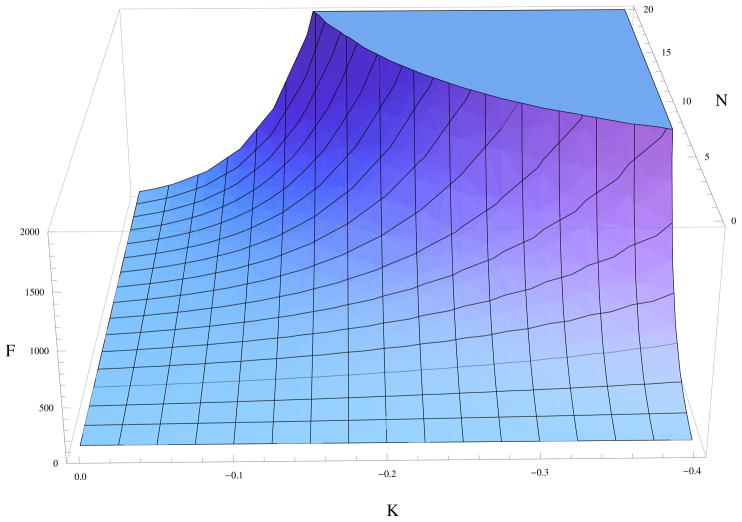
In Fig. (2), we look at properties of our model and how sensitive our model predictions are to the numerical value of K in general. We plot the variance over mean production squared of species A, a quantity we call F, within the interval [t,t + δt] given NA = 0 at time t. We define the mean production as 〈δNA〉 = 〈NA (t + δt) − NA (t)〉 and the variance as , where the subscript c denotes cumulants. These cumulants can be computed analytically, for example see Eq. (5). We plot , as a function of the number of N = NB proteins, and K. It shows that fluctuations in numbers of protein A grow dramatically larger either as the number, N, of proteins B increases or as the negative feedback is made stronger. The latter is expected for a bistable system.
Fig.2. Effect of negative feedback strength on production fluctuations of A.
Here we look at how F, production rate fluctuations normalized by its mean squared, varies with N and K using hα = hβ = −4.605, hA = hB = 7.60.
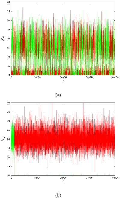
Fig. (3a) shows the Gillespie trajectory of the populations of states A and B over time, for a particular set of parameters. We then applied MaxCal to those trajectories to extract our Lagrange multipliers by the methods described above. Fig. (3b) shows the MaxCal model that we extracted. At a qualitative level, MaxCal captures well the two very different time scales: the fast fluctuations within each stable state of the system, and the much longer time scale over which transitions occur from one state to the other. It also captures the sharpness of the transitions between the two stable states. Comparing Fig. (4) to Figure (3) shows how even small changes in K in this model can dramatically change the qualitative system behavior. For example, as K becomes more positive (weakening the negative feedback), the transitions become much less sharp.
Fig.4. Correlation strength changes hopping dynamics.
Given the same Gillespie model as in Fig. (3a), if we now use a value of: (a) K 50% smaller(−0.19) or (b) 50% larger (−0.57) than those extracted by MaxCal, the predicted model behavior is very different.
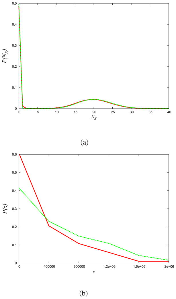
As a more quantitative test, Fig. (5a) shows that the MaxCal model correctly computes static properties such as the particle-number distribution functions around the two states. For the dynamics, Fig. (5b) shows that MaxCal also gives approximately correct dwell-time distributions, even over time scales that are much longer than those used to parametrize our model 2.
Fig.5. MaxCal predicts static and dynamical distribution functions.
(a) Distribution of particle numbers, (b) Distribution of dwell times. (Green) Gillespie ‘raw data’. (Red) Maximum Caliber model. Parameters are those used in Fig. (3).
For instance, MaxCal predicts an average dwell time of 〈 τ 〉 = 0.44 ±0.43 × 10⁶ s while the simulated data reveals average dwells of 〈 τ 〉 = 0.74 ±0.70 × 10⁶ s. The dwell time uncertainty is related to the inherent dwell-time-distribution variance, not a sampling error.
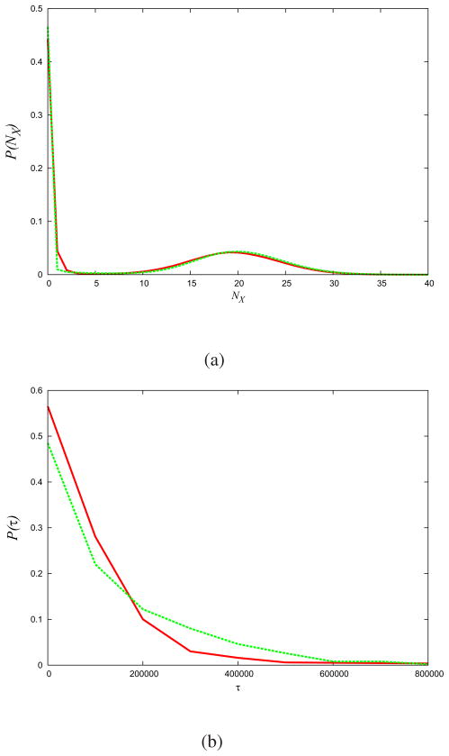
Figs. (6) and (7) are based on different parameter values: d = 0.005, k = 0.1, f = 100 and r = 2. In this case, the value of K = −0.295 that is extracted by MaxCal corresponds to a larger number of transitions between states per unit time. The average dwell time found by MaxCal is 〈τ〉 = 0.11 ± 0.11 × 10⁶s while for the simulated data it is 〈τ〉 = 0.16 ±0.17 × 10⁶s. As the binding-unbinding rates to the gene-promoter complex, f and r, are made large compared to typical birth-death rates, the predictions of MaxCal improve.
Fig.6. Gillespie and MaxCal time traces for a different parameter regime.
(a) Gillespie time trace. Gillespie model, using d = 0.005, k = 0.1, f = 100 and r = 2. (b) MaxCal model time trace. Corresponding MaxCal model with the extracted parameter K = −0.294 using hα = hβ = −4.605 and hA = hB = 7.6.
Fig. 7. Prediction of dynamical and static distrbutions for a different parameter regime.
(a) Distribution of particle numbers. (b) Distribution of dwell times. (Green) Gillespie simulations. (Red) MaxCal model. Parameters are those used in Fig. (6).
Within our MaxCal model, we have assumed that correlations happen essentially instantaneously, without time delays. However, real systems will have time delays. The approximation made in our current MaxCal model qualitatively breaks down when binding-unbinding events from the gene-promoter complex are slow compared to typical birth-death rates. For example, the agreement of Fig. (5b) was worse than that of Fig. (7). This is because there is a delay in the effect of species B on A, and vice versa, when binding-unbinding rates are not much faster than birth-death events.
We note here the importance of the dynamical fluctuations, relative to average properties. Suppose we take the average (mass-action) behavior of the same model of the ETS that we used in our Gillespie simulation above. The time evolution of the two species A and α would be given by
| (12) |
| (13) |
We neglect here terms in Eq. (12) that are due to binding and unbinding of A in the ETS to β because we assume there are a large number of A’s. In addition, we have assumed that there is a single α.
When binding and unbinding rates of A and B to the promoter, f and r respectively, are faster than production and degradation of A and B, then we can assume that 〈 α 〉 is in approximate equilibrium with 〈 α* 〉, so we have 〈 α̇ 〉 = 0. Combining Eq. (13) with Eq. (12) yields
| (14) |
The key point is that the mass-action dynamics predicted from Eq. (14) shows no bifurcation behavior [38]. The bistability in this system is a stochastic phenomenon that results from the small numbers of particles.
Our MaxCal approach bears some resemblance to maximum-likelihood (ML) methods. ML starts with knowledge of a reaction topology. ML expresses the probabilities of the various trajectories the system could take, given that reaction topology. ML then finds those parameters that maximize the probability of the experimentally observed path. MaxCal also enumerates all the possible trajectories of a system. However, MaxCal does not require prior knowledge of the reaction topology. In addition, MaxCal chooses parameters to ensure that the average rates of the model are identical to those of the experiments and gives a minimal model consistent with this data.
Conclusions
We have described how to apply the method of Maximum Caliber to model the time trajectories of bistable systems. As an illustration, we have considered the exclusive toggle switch (ETS) [38, 39], resembling the experimental system of Gardner et al. [34]. To create the “raw experimental data” trajectories, we simulated a model exclusive toggle switch using the Gillespie algorithm. We then applied the method of MaxCal, to see if it could properly extract the full dynamical and static behavior of the toggle switch.
MaxCal takes as input a few measured average quantities over the trajectories. It then computes a dynamical partition-function-like quantity. From that quantity, MaxCal then predicts other dynamical properties. We find that MaxCal produces a predictive underlying model for this stochastically driven bistable system. The advantages of the MaxCal approach are that: 1) it is more directly data-driven that other approaches, 2) the model is built using a minimal set of parameters(in our case we use less parameters than would have been used in the corresponding master equations for the toggle), 3) it is based on observable correlations between variables, rather than ad hoc functional forms, and 4) it captures the dynamical averages and fluctuations at both short and long time scales despite requiring only relatively short trajectories to predict quantities that would otherwise typically require much larger datasets. Also, as shown in Fig. (2), we find that switching behavior of the toggle switch correlates with conditions under which the fluctuations become unstable.
Supplementary Material
Acknowledgments
We appreciate the support of NIH grant GM34993, SP acknowledges the FQRNT for its financial support, KG acknowledges an FRF Grant from DU. We thank Adam Arkin for proposing the toggle switch as a test case; George Peterson, Julian Lee and Hao Ge for proofreading our manuscript; Attila Szabo and Rob Phillips for many interesting discussions.
Footnotes
In the experiments of Gardner et al. [34], the E. Coli in which are injected the engineered plasmid containing both promoters are replicating as the experiment is carried through. This set of chemical reactions above does not take this or other complications into account, rather the reactions put forth are a simple set of ingredients required to obtain bistable steady state as well as switching between such states.
The dwell times were obtained by determining levels of protein A and B at time intervals of length T in the time traces. If protein A had the higher level, then a counter is set to 1; otherwise it is 0. A switch is indicated by a change in the counter in the next interval. For sufficiently large T, there is a range over which the dwell times are independent of T. If T is too large, short transitions are missed. If T is too small, fluctuations are picked up as switches between steady states. It is because of the difficulty in defining what is a true transition in the presence of the rare raggedy switches that we define a switch through the simple algorithm above. Since we are really interested in comparing the dwells in MaxCal and Gillespie traces, to avoid bias, we use the same algorithm throughout with T equal to 1000 Gillespie or MaxCal steps, a step being defined by a change in particle number of A or B. We also verified our distribution of dwell times in different ways, for example by averaging levels of A and B within the interval T and using this to determine whether our counter variable should be set to 0 or 1. Different specialized methods for computing dwell times for toggle switches are also available in the literature [40].
Supporting Information Summary
The supporting information contains two sections. The first is a description of the method of Maximum Caliber. In particular, it contains a detailed derivation of the dynamical partition function. The second section shows under which circumstances the master equation and the dynamical partition function are related. This material is available free of charge via the Internet at http://pubs.acs.org.
References
- 1.Wernet MF, Mazzoni EO, Çelik A, Duncan DM, Duncan I, Desplan C. Nature. 2006;440:174–180. doi: 10.1038/nature04615. [DOI] [PMC free article] [PubMed] [Google Scholar]
- 2.Samoilov MS, Price G, Arkin AP. Science’s stke. 2006;366:re17. doi: 10.1126/stke.3662006re17. [DOI] [PubMed] [Google Scholar]
- 3.Smits WK, Kuipers OP, Veening JW. Nat Rev Micro. 2006;4:259–271. doi: 10.1038/nrmicro1381. [DOI] [PubMed] [Google Scholar]
- 4.Venning JW, Smits WK, Kuipers OP. Ann Rev Micro. 2008;62:193–210. doi: 10.1146/annurev.micro.62.081307.163002. [DOI] [PubMed] [Google Scholar]
- 5.Huang S, Guo YP, May G, Enver T. Dev Bio. 2007;305:695–713. doi: 10.1016/j.ydbio.2007.02.036. [DOI] [PubMed] [Google Scholar]
- 6.Maamar H, Raj A, Dubnau D. Science. 2007;317:526–529. doi: 10.1126/science.1140818. [DOI] [PMC free article] [PubMed] [Google Scholar]
- 7.Paliwal S, Iglesias PA, Campbell K, Hilioti Z, Groisman A, Levchenko A. Nature. 2007;446:46–51. doi: 10.1038/nature05561. [DOI] [PubMed] [Google Scholar]
- 8.Veening JW, Hamoen LW, Kuipers OP. Mol Micro. 2005;56:1481–1494. doi: 10.1111/j.1365-2958.2005.04659.x. [DOI] [PubMed] [Google Scholar]
- 9.Bagowski CP, Ferrell JE., Jr Current Bio. 2001;11:1176–1182. doi: 10.1016/s0960-9822(01)00330-x. [DOI] [PubMed] [Google Scholar]
- 10.Acar M, Mettetal JT, van Oudenaarden A. Nat Gen. 2008;40:471–475. doi: 10.1038/ng.110. [DOI] [PubMed] [Google Scholar]
- 11.Hooshangi S, Thiberge S, Weiss R. Proc Natl Acad Sci USA. 2005;102:3581–3586. doi: 10.1073/pnas.0408507102. [DOI] [PMC free article] [PubMed] [Google Scholar]
- 12.Huang CY, Ferrell JE., Jr Proc Natl Acad Sci USA. 1996;93:10078–10083. doi: 10.1073/pnas.93.19.10078. [DOI] [PMC free article] [PubMed]
- 13.van Kampen NG. Stochastic Processes in Chemistry and Physics. North Holland Publishing Company; Amsterdam: 1981. [Google Scholar]
- 14.Gillepsie DT. J Phys Chem. 1977;81:2340–2361. [Google Scholar]
- 15.Arkin A, Ross J. J Phys Chem. 1995;99:970–979. [Google Scholar]
- 16.Ross J. Acc Chem Res. 2003;36:839–847. doi: 10.1021/ar020285f. [DOI] [PubMed] [Google Scholar]
- 17.Noé F. J Chem Phys. 2008;128:244103. doi: 10.1063/1.2916718. [DOI] [PubMed] [Google Scholar]
- 18.Milescu LS, Akk G, Sachs F. Biophys J. 2005;88:2494–2515. doi: 10.1529/biophysj.104.053256. [DOI] [PMC free article] [PubMed] [Google Scholar]
- 19.McKinney SA, Joo C, Ha T. Biophys J. 2006;91:1941–1951. doi: 10.1529/biophysj.106.082487. [DOI] [PMC free article] [PubMed] [Google Scholar]
- 20.Witkoskie JB, Cao J. J Chem Phys. 2004;121:6361–6372. doi: 10.1063/1.1785783. [DOI] [PubMed] [Google Scholar]
- 21.Flomenbom O, Klafter J, Szabo A. Biophys J. 2005;88:3780–3783. doi: 10.1529/biophysj.104.055905. [DOI] [PMC free article] [PubMed] [Google Scholar]
- 22.Gull SF. In: Bayesian Inductive Inference and Maximum Entropy, Maximum Entropy and Bayesian Methods in Science and Engineering. Erickson GJ, Smith CR, editors. Vol. 1. Kluwer Academic Publishers; Boston: 1988. pp. 53–74. [Google Scholar]
- 23.Kienker P. Roy Soc London Series B. 1989;236:269–309. doi: 10.1098/rspb.1989.0024. [DOI] [PubMed] [Google Scholar]
- 24.Jaynes ET. In: ‘Macroscopic Prediction,’ in Complex Systems - Operational Approaches. Haken H, editor. Springer-Verlag; Berlin: 1985. p. 254. [Google Scholar]
- 25.Bretthorst GL, Jaynes ET. Probability Theory: The Logic of Science. Cambridge University Press; 2003. [Google Scholar]
- 26.Jaynes ET. Phys Rev. 1957;108:171–190. [Google Scholar]
- 27.Jaynes ET. In: Annual Review of Physical Chemistry. Rabinovitch S, editor. Annual Reviews Ins; Palo Alto: 1980. pp. 579–601. [Google Scholar]
- 28.Ghosh K, Dill KA, Inamdar MM, Seitaridou E, Phillips R. Am J Phys. 2006;74:123–133. doi: 10.1119/1.2142789. [DOI] [PMC free article] [PubMed] [Google Scholar]
- 29.Seitaridou E, Inamdar M, Phillips R, Ghosh K, Dill K. J Phys Chem B. 2007;111:2288–2292. doi: 10.1021/jp067036j. [DOI] [PMC free article] [PubMed] [Google Scholar]
- 30.Wu D, Ghosh K, Inamdar M, Lee HJ, Fraser S, Dill K, Phillips R. Phys Rev Lett. 2009;103:050603. doi: 10.1103/PhysRevLett.103.050603. [DOI] [PMC free article] [PubMed] [Google Scholar]
- 31.Pressé S, Ghosh K, Phillips R, Dill K. Phys Rev E. 2010;82:031905. doi: 10.1103/PhysRevE.82.031905. [DOI] [PubMed] [Google Scholar]
- 32.Stock G, Ghosh K, Dill K. J Chem Phys. 2008;128:194102. doi: 10.1063/1.2918345. [DOI] [PMC free article] [PubMed] [Google Scholar]
- 33.Otten M, Stock G. J Chem Phys. 2010;133:034119. doi: 10.1063/1.3455333. [DOI] [PubMed] [Google Scholar]
- 34.Gardner TS, Cantor CR, Collins JJ. Nature. 2000;403:339–342. doi: 10.1038/35002131. [DOI] [PubMed] [Google Scholar]
- 35.Tozaki H, Kobayashi TJ, Okano H, Yamamoto R, Aihara K, Kimura H. FEBS Lett. 2008;582:1067–1072. doi: 10.1016/j.febslet.2008.02.057. [DOI] [PubMed] [Google Scholar]
- 36.Atkinson MR, Savageau MA, Myers JT, Ninfa AJ. Cell. 2003;113:597–607. doi: 10.1016/s0092-8674(03)00346-5. [DOI] [PubMed] [Google Scholar]
- 37.Kim K, Wang J. PLoS Comp Bio. 2007;3:e60. doi: 10.1371/journal.pcbi.0030060. [DOI] [PMC free article] [PubMed] [Google Scholar]
- 38.Lipshtat A, Loinger A, Balaban NQ, Biham O. Phys Rev Lett. 2006;96:188101. doi: 10.1103/PhysRevLett.96.188101. [DOI] [PubMed] [Google Scholar]
- 39.Loinger A, Biham O. Phys Rev Lett. 2009;103:068104. doi: 10.1103/PhysRevLett.103.068104. [DOI] [PubMed] [Google Scholar]
- 40.Allen RJ, Warren PB, ten Wolde PR. Phys Rev Lett. 2005;94:018104. doi: 10.1103/PhysRevLett.94.018104. [DOI] [PubMed] [Google Scholar]
Associated Data
This section collects any data citations, data availability statements, or supplementary materials included in this article.


