Sensitivity, robustness, and identifiability in stochastic chemical kinetics models

Abstract

We present a novel and simple method to numerically calculate Fisher information matrices for stochastic chemical kinetics models. The linear noise approximation is used to derive model equations and a likelihood function that leads to an efficient computational algorithm. Our approach reduces the problem of calculating the Fisher information matrix to solving a set of ordinary differential equations. This is the first method to compute Fisher information for stochastic chemical kinetics models without the need for Monte Carlo simulations. This methodology is then used to study sensitivity, robustness, and parameter identifiability in stochastic chemical kinetics models. We show that significant differences exist between stochastic and deterministic models as well as between stochastic models with time-series and time-point measurements. We demonstrate that these discrepancies arise from the variability in molecule numbers, correlations between species, and temporal correlations and show how this approach can be used in the analysis and design of experiments probing stochastic processes at the cellular level. The algorithm has been implemented as a Matlab package and is available from the authors upon request.

Understanding the design principles underlying complex biochemical networks cannot be grasped by intuition alone (1). Their complexity implies the need to build mathematical models and tools for their analysis. One of the powerful tools to elucidate such systems’ performances is sensitivity analysis (2). Large sensitivity to a parameter suggests that the system’s output can change substantially with small variation in a parameter. Similarly large changes in an insensitive parameter will have little effect on the behavior. Traditionally, the concept of sensitivity has been applied to continuous deterministic systems described by differential equations to identify which parameters a given output of the system is most sensitive to; here, sensitivities are computed via the integration of the linearization of the model parameters (2).

In modeling biological processes, however, recent years have have witnessed rapidly increasing interest in stochastic models (3), as experimental and theoretical investigations have demonstrated the relevance of stochastic effects in chemical networks (4, 5). Although stochastic models of biological processes are now routinely being applied to study biochemical phenomena ranging from metabolic networks to signal transduction pathways (6), tools for their analysis are in their infancy compared to the deterministic framework. In particular, sensitivity analysis in a stochastic setting is usually, if at all, performed by analysis of a system’s mean behavior or using computationally intensive Monte Carlo simulations to approximate finite differences of a system’s output or the Fisher information matrix with associated sensitivity measures (7, 8). The Fisher information has a prominent role in statistics and information theory: It is defined as the variance of the score and therefore allows us to measure how reliably inferences are. Geometrically, it corresponds to the curvature around the maximum value of the log likelihood.

The interest in characterizing the parametric sensitivity of the dynamics of biochemical network models has two important reasons. First, sensitivity is instrumental for deducing system properties, such as robustness (understood as stability of behavior under simultaneous changes in model parameters) (9). The concept of robustness is of significance, in turn, as it is related to many biological phenomena such as canalization, homeostasis, stability, redundancy, and plasticity (10). Robustness is also relevant for characterizing the dependence between parameter values and system behavior. For instance, it has recently been reported that a large fraction of the parameters characterizing a dynamical system are insensitive and can be varied over orders of magnitude without significant effect on system dynamics (11–13).

Second, methods for optimal experimental design use sensitivity analysis to define the conditions under which an experiment is to be conducted to maximize the information content of the data (14). Similarly, identifiability analysis uses the concept of sensitivity to determine a priori whether certain parameters can be estimated from experimental data of a given type (15).

We use the linear noise approximation (LNA) as a continuous approximation to Markov jump processes defined by the chemical master equation (CME). This approximation has previously been used successfully for modeling as well as for inference (16, 17, 18). Applying the LNA allows us to represent the Fisher information matrix (FIM) as a solution of a set of ordinary differential equations (ODEs). We use this framework to investigate model robustness, study the information content of experimental samples and calculate Cramér–Rao (CR) bounds for model parameters. Analysis is performed for time series (TS) and time point (TP) data as well as for a corresponding deterministic (DT) model. Results are compared with each other and provide novel insights into the consequences of stochasticity in biochemical systems. Two biological examples are used to demonstrate our approach and its usefulness: a simple model of gene expression and a model of the p53 system. We show that substantial differences in the structure of FIMs exist between stochastic and deterministic versions of these models. Moreover, discrepancies appear also between stochastic models with different data types (TS, TP), and these can have significant impact on sensitivity, robustness, and parameter identifiability. We demonstrate that differences arise from general variability in the number of molecules, correlation between them, and temporal correlations.

Chemical Kinetics Models

We consider a general system of N chemical species inside a fixed volume and let x = (x₁,…,x_N)^T denote the number of molecules. The stoichiometric matrix S = {s_ij}_{i=1,2…N;j=1,2…R} describes changes in the population sizes due to R different chemical events, where each s_ij describes the change in the number of molecules of type i from X_i to X_i + s_ij caused by an event of type j. The probability that an event of type j occurs in time interval [t,t + dt) equals f_j(x,Θ,t)dt. The functions f_j(x,Θ,t) are called transition rates and Θ = (θ₁,…,θ_L) is a vector of model parameters. This specification leads to a Poisson birth and death process with transition densities described by the CME (see SI Appendix). Unfortunately, the CME is not easy to analyze and hence various approximations have been developed. As shown in refs. 16–19, the linear noise approximation provides a useful and reliable framework for both modeling and statistical inference. It is valid for systems with large number of reacting molecules and is an analogy of the central limit theorem for Markov jump processes defined by CME (20). Biochemical reactions are modeled through a stochastic dynamic model that essentially approximates a Poisson process by an ODE model with an appropriately defined noise process. Within the LNA a kinetic model is written as:

[1]

[2]

[3]

where

[4]

[5]

[6]

Eq. [1] divides the system’s state into a macroscopic state, φ(t) = (ϕ₁(t),…,ϕ_N(t)), and random fluctuations, ξ(t). The macroscopic state is described by an ODE [2], the macroscopic rate equation (MRE), which in general needs to be solved numerically. Stochastic fluctuations ξ are governed by a Wiener process (dW) driven linear stochastic differential Eq. [3] with an explicit solution readily available (see SI Appendix). The variance V(t) of the system’s state x can be explicitly written in terms of an ODE

[7]

which is equivalent to the fluctuation-dissipation theorem. Similarly, temporal covariances are given by

[8]

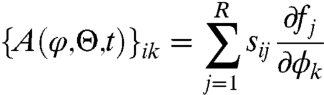
where Φ(s,t) is the fundamental matrix of the nonautonomous system of ODEs

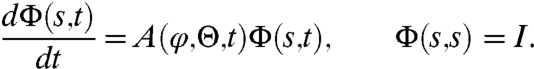[9]

Eqs. [1]–[9] are used to derive the likelihood of experimental data. To account for different experimental settings we consider three types of data: time-series (TS), time-point (TP), and deterministic (DT). For TS measurements are taken from a single trajectory (following the same cell) and therefore are statistically dependent; in practice TS data are usually obtained using fluorescent microscopy. TP measurements at each time point are taken from different trajectories (end time points of trajectories following different cells) and are thus independent. These data reflect experimental setups where the sample is sacrificed and the sequence of measurements is not strictly associated with the same sample path (e.g., flow-cytometry, quantitative polymerase chain reaction). DT data are defined as a solution of MRE [2] with normally distributed measurement error with zero mean and variance and refer to measurements averaged over population of cells.

Suppose measurements are collected at times t₁,…,t_n. For simplicity we consider the case where at each time point t_i all components of x_i are measured. In the SI Appendix, we demonstrate that the same analysis can be done for a model with unobserved variables at no extra cost other than more complex notation. First let x_Q ≡ (x_t1,…,x_tn) be an nN column vector that contains all measurements of type Q, where Q∈{TP,TS,DT}. It can be shown (see SI Appendix) that

[10]

where MVN denotes the multivariate normal distribution,

[11]

and is a solution of the MRE [2] such that 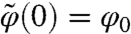and Σ_Q is a (nN) × (nN) symmetric block matrix Σ_Q(Θ) = {Σ_Q(Θ)^(i,j)}_{i=1,…,N;j=1,…,N} such that

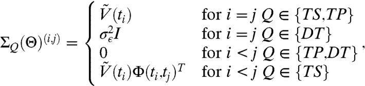[12]

and is a solution of Eq. [7] for a given initial condition . The MVN likelihood is a result of our LNA and is analogous to the central limit theorem for the CME. It is valid under the assumption of large number of molecules reacting in the system (20).

Fisher Information Matrix

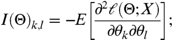
To calculate the FIM^† for the model [1]–[3], first, suppose that a random variable X has an N-variate normal distribution with density ψ, mean μ(Θ) = (μ₁(Θ),…,μ_N(Θ))^T, and covariance matrix Σ(Θ). The FIM is then defined (21) as I(Θ) = {I(Θ)_k,l}_k,l=1,…,L, where

[13]

Then I(Θ)_i,j can be expressed as

[14]

The above formula shows that, to calculate FIM for a multivariate normal distribution, it is enough to calculate the covariance matrix Σ(θ), parameter derivatives of mean and parameter derivatives of the covariance matrix .

In the LNA Eqs. [11] and [12] describe mean and variance, respectively, of experimental measurements, x_Q. The mean is given as the solution of an ODE, and the variance is either given as a product of solutions of ODEs (TS), directly as a solution of an ODE [7] (TP), or is simply constant (DT). Hence, to calculate the FIM we calculate the derivatives of the solutions of an ODE with respect to the parameters (22). For illustration, consider an N dimensional ODE

[15]

where θ is a scalar parameter. Denote by the solution of Eq. [15] with initial condition z₀ and let . It can be shown that ζ satisfies (22)

[16]

where is the Jacobian . We can thus calculate derivatives , , and that give and needed to compute FIM for the model [1]–[3] (see SI Appendix).

The FIM is of special significance for model analysis as it constitutes a tool for sensitivity analysis, robustness, identifiability, and optimal experimental design as we will show below.

The FIM and Sensitivity.

The classical sensitivity coefficient for an observable Q and parameter θ is

The behavior of a stochastic system is defined by observables that are drawn from a probability distribution. The FIM is a measure of how this distribution changes in response to infinitesimal changes in parameters. Suppose that ℓ(Θ; X) = log(ψ(X,Θ)) and ℓ(Θ) = -E[ℓ(Θ; X)]. Then,

[17]

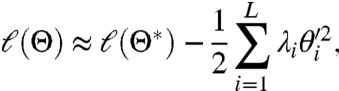
i.e., the FIM is the expected Hessian of ℓ(Θ,X). Therefore, if Θ^∗ is the maximum likelihood estimate of a parameter there is a L × L orthogonal matrix C such that, in the new parameters θ^′ = C(Θ - Θ^∗),

[18]

for Θ near Θ^∗. From this it follows that the λ_i are the eigenvalues of the FIM and that the matrix C diagonalizes it. If we assume that the λ_i are ordered so that λ₁≥⋯≥λ_L, then it follows that around the maximum the likelihood is most sensitive when is varied and least sensitive when is varied, and λ_i is a measure of this. Because , we can regard C_ij as the contribution of the parameter θ_j to varying and thus

[19]

can be regarded as a measure of the sensitivity of the system to θ_j. It is sometimes appropriate to normalize this and instead consider

[20]

Robustness.

Related to sensitivity, robustness in systems biology is usually understood as persistence of a system to perturbations to external conditions (23). Sensitivity considers perturbation in a single parameter whereas robustness takes into account simultaneous changes in all model parameters. Near to the maximum Θ^∗ the regions of high expected log-likelihood ℓ(Θ)≥ℓ(Θ^∗) - ε are approximately the ellipsoids NS(Θ^∗,ε) given by the equation

[21]

The ellipsoids have principal directions given by eigenvectors C and equatorial radii . Sets NS are called neutral spaces as they describe regions of parameter space in which a system’s behavior does not undergo significant changes (10) and arise naturally in the analysis of robustness.

Confidence Intervals and Asymptotics.

The asymptotic normality of maximum likelihood estimators implies that if Θ^∗ is a maximum likelihood estimator then the NS describe confidence ellipsoids for Θ with confidence levels corresponding to ε. The equatorial radii decrease naturally with the square root of the sample size (24).

Parameter Identifiability and Optimal Experimental Design.

The FIM is of special significance for model analysis as it constitutes a classical criterion for parameter identifiability (15). There exist various definitions of parameter identifiability and here we consider local identifiability. The parameter vector Θ is said to be (locally) identifiable if there exists a neighborhood of Θ such that no other vector Θ^∗ in this neighborhood gives raise to the same density as Θ(15). Formula [18] implies that Θ is (structurally) identifiable if and only if FIM has a full rank (15). Therefore the number of nonzero eigenvalues of FIM is equal to the number of identifiable parameters, or more precisely, to the number of identifiable linear combinations of parameters.

The FIM is also a key tool to construct experiments in such a way that the parameters can be estimated from the resulting experimental data with the highest possible statistical quality. The theory of optimal experimental design uses various criteria to asses information content of experimental sampling methods; among the most popular are the concepts of D-optimality that maximizes the determinant of FIM, and A-optimality that minimize the trace of the inverse of FIM (14). Diagonal elements of the inverse of FIM constitute a lower-bound for the variance of any unbiased estimator of elements of Θ; this is known as the Cramér–Rao inequality (see SI Appendix). Finally, it is important to keep in mind that some parameters may be structurally identifiable, but not be identifiable in practice due to noise; these would correspond to small but nonzero eigenvalues of the FIM. Maximizing the number of eigenvalues above some threshold that reflects experimental resolution, may therefore be a further criterion to optimize experimental design. But all of these criteria revolve around being able to evaluate the FIM.

Results

To demonstrate the applicability of the presented methodology for calculation of FIMs for stochastic models we consider two examples: a simple model of single gene expression, and a model of the p53 system. The simplicity of the first model allows us to explain how the differences between deterministic and stochastic versions of the model as well as TS and TP data arise. In the case of the p53 system model the informational content, as well as sensitivities and neutral spaces are compared between TS, TP, and DT data.

Single Gene Expression Model.

Although gene expression involves numerous biochemical reactions, the currently accepted consensus is to model it in terms of only three biochemical species (DNA, mRNA, and protein) and four reaction channels (transcription, mRNA degradation, translation, and protein degradation) (e.g., refs. 12 and 25). Such a simple model has been used successfully in a variety of applications and can generate data with the same statistical behavior as more complicated models (26, 27). We assume that the process begins with the production of mRNA molecules (r) at rate k_r. Each mRNA molecule may be independently translated into protein molecules (p) at rate k_p. Both mRNA and protein molecules are degraded at rates γ_r and γ_p, respectively. Therefore, we have the state vector x = (r,p), and reaction rates corresponding to transcription of mRNA, translation, degradation of mRNA, and degradation of protein.

[22]

Identifiability Study.

In a typical experiment, only protein levels are measured (17, 28). It is not entirely clear a priori what parameters of gene expression can be inferred; it is also not obvious if and how the answer depends on the nature of the data (i.e., TS, TP, or DT). We address these questions below.

We assumed that the system has reached the unique steady state defined by the model and that only protein level is measured either as TS

[23]

or as TP

[24]

where the upper indices for TP measurements denote the number of trajectories from which the measurement have been taken to emphasize independence of measurements. Results of the analysis are presented in Table S2. For TS data we have four identifiable parameters whereas time-point measurements provide enough information to estimate only two parameters. To some extent this makes intuitive sense: TS data contain information about mean, variance, and autocorrelation functions, which can be very sensitive to changes in degradation rates; TP measurements reflect only information about mean and variance of protein levels therefore only two parameters are identifiable. On the other hand, TP measurements provide independent samples that is reflected in lower Cramér–Rao bounds. Table S2 also contains a comparison with the corresponding deterministic model. As one might expect in the deterministic model only one parameter is identifiable as the mean is the only quantity that is described by the deterministic model, and parameter estimates are informed neither by variability nor by autocorrelation.

Perturbation Experiment.

To demonstrate that identifiability is not a model specific but rather an experiment specific feature, we performed a similar analysis as above for the same model with the same parameters but with the fivefold increased initial mean and 25-fold increased initial variance. Results are presented in Table S3. Some of the conclusions that can be made are hard to predict without calculating the FIM. The amount of information in TS data is now much larger than in TP data (higher determinant) and also CR bounds are now much lower for TP than for TS data. CR bounds for TS and TP are substantially lower than for the steady state data (except k_r). Interestingly, all four parameters can be inferred from TS and TP data, but not in the deterministic scenario. For steady state data all parameters could only be inferred from TS data (Table S3).

Maximizing the Information Content of Experimental Data.

The amount of information in a sample does not depend solely on the type of data (TS, TP), but also on other factors that can be controlled in an experiment. One easily controllable quantity is the sampling frequency Δ. We consider here only equidistant sampling and keep number of measurements constant. Therefore we define Δ as time between subsequent observations Δ = t_i+1 - t_i. To show how sampling frequency influences informational content of a sample for the model of gene expression we used four parameter sets (Table S1) and assumed that the data have the form [23]. The amount of information in a sample was understood as the determinant of the FIM, equivalent to the product of the eigenvalues of the FIM. Results in Fig. 1 demonstrate that our method can be used to determine optimal sampling frequency, given that at least some rough estimates of model parameters are known. It is worth noting that equidistant sampling is not always the best option and more complex strategies have been proposed in experimental design literature.

Fig. 1.

Determinant of FIM plotted against sampling frequency Δ (in hours). We used logarithms of four parameter sets (see Table S1). Sets 1 and 3 correspond to slow protein degradation (γ_p = 0.7); and sets 2 and 4 describe fast protein degradation (γ_p = 1.2). We assumed that 50 measurements (n = 50) of protein levels were taken from the stationary state. Observed maximum in information content results from the balance between independence and correlation of measurements.

Differences in Sensitivity and Robustness Analysis in TS, TP, and DT Versions of the Model.

TS, TP, and DT versions of the model differ when one considers information content of samples, and such discrepancies exist also when sensitivity and robustness are studied. First, deterministic models completely neglect variability in molecular species. Variability, however, is a function of parameters, and like the mean, is sensitive to them. Second, deterministic models do not include correlations between molecular species. Third, temporal correlations are neglected in TP and DT models. To understand these effects we first analyze the analytical form of means, variances, and correlations for this model (see SI Appendix). We start with the effect of incorporating variability. Suppose we consider a change in parameters; e.g., k_p, γ_p by a factor δ (k_p,γ_p) → (k_p + δk_p,γ_p + δγ_p). The means of RNA and protein concentrations are not affected by this perturbation, whereas the protein variance does change (see formulas [33]–[37] in SI Appendix). This result is related to the number of nonzero eigenvalues of the FIM. The FIM for the stationary distribution of this model with respect to parameters k_p, γ_p has only one positive eigenvalue for the deterministic model and two positive eigenvalues for the stochastic model.

To study the effect of correlation between RNA and protein levels ρ_rp we first note that formulas [33]–[37] in the SI Appendix demonstrate that at constant mean, correlation increases with γ_p when accompanied by a compensating increase in k_p. Fig. 2 (left column) presents neutral spaces (21) for parameter pairs for different values of correlation, ρ_rp. The differences between DT and TS are enhanced by the correlation.

Fig. 2.

Neutral spaces for TS and DT versions of the model of single gene expression for logs of parameters k_r and γ_p. (Left) Differences resulting from RNA, protein correlation: ρ_rp = 0.1 (Top) ρ_rp = 0.5 (Middle), ρ_rp = 0.9 (Bottom). Correlation 0.5 corresponds to parameter set 3 from Table S1 and was varied by equal-scaling of parameters k_p, γ_p. (Right) Differences resulting from temporal correlations. We assumed n = 50 and tuned correlation between observation by changing sampling frequency Δ = 0.3 h (Left) Δ = 3 h (Center) Δ = 30 h (Right). Set 3 of parameters was used (Table S1).

Similar analysis reveals that taking account of the temporal correlations also changes the way the model responds to parameter perturbations. Fig. 2 (right column) shows neutral spaces for three different sampling frequencies and indicates that the differences between stochastic and deterministic models decrease with Δ.

Model of p53 System.

The model of single gene expression is a linear model with only four parameters and a simple stationary state and illustrates how the methodology can be used to provide relevant conclusions and investigate discrepancies between sensitivities of TS, TP, and DT models. Our methodology, however, can also be used to study more complex models, and here we have chosen the p53 signalling system, which incorporates a feedback loop between the tumor suppressor p53 and the oncogene Mdm2, and is involved in regulation of cell cycle and response to DNA damage.

We use the model introduced in ref. 29 that reduces the system to three molecular species, p53, mdm2 precursor, and mdm2, denoted here by p, y₀ and y, respectively. The state of the system is therefore given by x = (p,y₀,y), and the deterministic version of the model can be formulated in terms of macroscopic rate equations

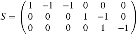[25]

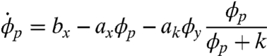[26]

[27]

[28]

Informational Content of TS and TP Data for the p53 System.

In the case of the single gene expression model we have argued that TS data are more informative due to accounting for temporal correlations. On the other hand, TP measurements provide statistically independent samples, which should increase informational content of the data. Therefore it is not entirely clear what data type is better for a particular parameter. If, for instance, a parameter is entirely informed by a system’s mean behavior than TP data will be more informative because TP data provide statistically independent samples about the mean. Whereas if a parameter is also informed by temporal correlations, then TS data will turn out to be more informative. It is difficult to predict a priori which effect will be dominating. Therefore calculation of FIM and comparison of their eigenvalues and diagonal elements is necessary. Eigenvalues and diagonal elements of FIMs calculated for parameters presented in Table S4 are plotted in Fig. S1 and Fig. 3, respectively. Eigenvalues of the FIM for TS data are larger than for TP data. Similarly, diagonal elements for all parameters are larger for TP than for TS data for most parameters difference is substantial. This indicates that temporal correlation is a sensitive feature of this system and provides significant information about model parameters. The lower information content of the TP data can, however, be compensated for by increasing the number of independent measurements, which is easily achievable in current experimental settings (see Fig. S2). For deterministic models the absolute value of elements of FIM depends on measurement error variance and therefore FIMs of TS and TP data can not be directly compared with the DT model.

Fig. 3.

(Left) Diagonal elements of FIM for TS and TP versions of p53 model. Values of FIM for DT verison are not presented as they can not be compared with those for stochastic models. (Right) Sensitivity coefficients for TS, TP, DT version of p53 model. FIMs were calculated for parameters presented in Table S4.

Sensitivity.

The sensitivity coefficients for TS, TP, and DT data are presented in Fig. 3. Despite differences outlined previously, here sensitivity coefficients are quite similar for all three types suggesting that the hierarchy of sensitive parameters is to a considerable degree independent on the type of data. The differences exist, however, in contributions (see Fig. S3), suggesting discrepancies in neutral spaces and robustness analysis that we present below.

Neutral Spaces.

Comparison of the neutral spaces [21] for each pair of data types and for each pair of the parameters are given in Fig. 4 and Figs. S4–S6. The conclusion we can draw from these figures is that NSs for TS, TP, and DT model exhibit substantial differences; these differences, however, are limited to certain parameter pairs. Differences between NPs of TS and DT models are exhibited in pairs involving parameters b_x, a_y; between TS and TP in pairs involving b_x; and between TP and DT also pairs involving b_x.

Fig. 4.

Neutral spaces for TS, TP, and DT versions of p53 model for logs of two parameter pairs (a₀,a_k) and (b_x,a_y). The left column presents differences resulting form general variability, correlations between species and temporal correlation (comparison of TS and TP models). The right column shows differences due to variability and correlation between species (comparison of TS and TP models). The top row is an example of parameters for which differences are negligible, bottom row presents a parameter pair with substantial differences. FIM was calculated for 30 measurements of all model variables and Δ = 1 h.

This suggests that parameter b_x is responsible either for the variability in molecular numbers or the correlation between species, as these are responsible for differences between TP and DT models. Similarly the lack of differences in pairs involving a_y in comparisons of TP and DT, and their presence in comparison of TP and TS indicates that parameter a_y is responsible for regulating the temporal correlations. This analysis agrees with what one might intuitively predict. Parameter b_x describes the production rate, and therefore the mean expression level of p53, and also the variability of all components of the system. It is difficult, however, to say how this parameter influences correlations between species. Parameter a_y, on the other hand, is the degradation rate of mdm2 and therefore clearly determines the temporal correlation of not only mdm2 but also of p53, because mdm2 regulates the degradation rate of p53. While heuristic, our analysis of the neutral spaces nevertheless clearly demonstrates the differences between the three types of models and creates a theoretical framework for investigating the role of parameters in the stochastic chemical kinetics systems and without the need to perform Monte Carlo sampling or other computationally expensive schemes.

Discussion

The aim of this paper was to introduce an innovative theoretical framework that allows us to gain insights into sensitivity and robustness of stochastic reaction systems through analysis of the FIM. We have used the linear noise approximation (16, 17, 30) to model means, variances, and correlations in terms of appropriate ODEs. Differentiating the solution of these ODEs with respect to parameters (22) allowed us to numerically calculate derivatives of means, variances, and correlations, which combined with the normal distribution of model variables implied by the LNA gave us the representation of the FIM in terms of solutions of ODEs. To our knowledge, no other method computes FIM for stochastic chemical kinetics models without the need for Monte Carlo simulations.

Given the role of the FIM in model analysis and increasing interest in stochastic models of biochemical reactions, our approach is widely applicable. It is primarily aimed at optimizing or guiding experimental design, and here we have shown how it can be used to test parameter identifiability for different data types, determine optimal sampling frequencies, examine information content of experimental samples and calculate Cramér–Rao bounds for kinetic parameter estimates. Its applicability, however, extends much further: it can provide a rationale as to which variables should be measured experimentally, or what perturbation should be applied to a system to obtain relevant information about parameters of interest. Similar strategies can also be employed to optimize model selection procedures. As demonstrated here, stochastic data incorporating information about noise structure are more informative and therefore experimental optimization for stochastic models models may be advantageous over similar methods for deterministic models.

A second topical application area is the study of robustness of stochastic systems. Interest in robustnesses results from the observation that biochemical systems exhibit surprizing stability in function under various environmental conditions. For deterministic models this phenomenon has been partly explained by the existence of regions in parameter space (neutral spaces) (10), in which perturbations to parameters do not result in significant changes in system output. We have demonstrated that even a very simple stochastic linear model of gene expression exhibits substantial differences when its neutral spaces are compared with the deterministic counterpart. Therefore a stochastic system may respond differently to changes in external conditions than the corresponding deterministic model. Our study presents examples of changes in parameters that do not affect behavior of a deterministic systems but may substantially change a probability distribution that defines the behavior of the corresponding stochastic system. Thus for systems in which stochasticity plays an important role random effects can not be neglected when considering issues related to robustness. More information regarding applicability of our method is available in the SI Appendix and Figs. S7–S13.

References

- 1.Csete ME, Doyle JC. Reverse engineering of biological complexity. Science. 2002;295:1664–1669. doi: 10.1126/science.1069981. [DOI] [PubMed] [Google Scholar]
- 2.Varma A, Morbidelli M, Wu H. Parametric Sensitivity in Chemical Systems. Cambridge, UK: Cambridge University Press; 1999. [Google Scholar]
- 3.Maheshri N, O’Shea EK. Living with noisy genes: How cells function reliably with inherent variability in gene expression. Annu Rev Bioph Biom. 2007;36:413–434. doi: 10.1146/annurev.biophys.36.040306.132705. [DOI] [PubMed] [Google Scholar]
- 4.McAdams HH, Arkin A. Stochastic mechanisms in gene expression. Proc Natl Acad Sci USA . 1997;94:814–819. doi: 10.1073/pnas.94.3.814. [DOI] [PMC free article] [PubMed] [Google Scholar]
- 5.Elowitz MB, Levine AJ, Siggia ED, Swain PS. Stochastic gene expression in a single cell. Science. 2002;297:1183–1186. doi: 10.1126/science.1070919. [DOI] [PubMed] [Google Scholar]
- 6.Wilkinson DJ. Stochastic modelling for quantitative description of heterogeneous biological systems. Nat Rev Genet. 2009;10:122–133. doi: 10.1038/nrg2509. [DOI] [PubMed] [Google Scholar]
- 7.Gunawan R, Cao Y, Petzold L, Doyle FJ., III Sensitivity analysis of discrete stochastic systems. Biophys J. 2005;88:2530–2540. doi: 10.1529/biophysj.104.053405. [DOI] [PMC free article] [PubMed] [Google Scholar]
- 8.Rathinam M, Sheppard PW, Khammash M. Efficient computation of parameter sensitivities of discrete stochastic chemical reaction networks. J Chem Phys. 2010;132:034103. doi: 10.1063/1.3280166. [DOI] [PMC free article] [PubMed] [Google Scholar]
- 9.Rand DA. Mapping the global sensitivity of cellular network dynamics. J R Soc Interface. 2008;5:S59–S69. doi: 10.1098/rsif.2008.0084.focus. [DOI] [PMC free article] [PubMed] [Google Scholar]
- 10.Daniels BC, Chen YJ, Sethna JP, Gutenkunst RN, Myers CR. Sloppiness, robustness, and evolvability in systems biology. Curr Opin Biotech. 2008;19:389–395. doi: 10.1016/j.copbio.2008.06.008. [DOI] [PubMed] [Google Scholar]
- 11.Brown KS, Sethna JP. Statistical mechanical approaches to models with many poorly known parameters. Phys Rev E. 2003;68:021904. doi: 10.1103/PhysRevE.68.021904. [DOI] [PubMed] [Google Scholar]
- 12.Rand DA, Shulgin BV, Salazar D, Millar AJ. Uncovering the design principles of circadian clocks: Mathematical analysis of flexibility and evolutionary goals. J Theor Biol. 2006;238:616–635. doi: 10.1016/j.jtbi.2005.06.026. [DOI] [PubMed] [Google Scholar]
- 13.Erguler K, Stumpf MPH. Practical limits for reverse engineering of dynamical systems: A statistical analysis of sensitivity and parameter inferability in systems biology models. Mol Biosyst. 2011;7:1595–1602. doi: 10.1039/c0mb00107d. [DOI] [PubMed] [Google Scholar]
- 14.Emery AF, Nenarokomov AV. Optimal experiment design. Meas Sci Technol. 1998;9:864–876. [Google Scholar]
- 15.Rothenberg TJ. Identification in parametric models. Econometrica. 1971;39:577–591. [Google Scholar]
- 16.Elf J, Ehrenberg M. Fast evaluation of fluctuations in biochemical networks with the linear noise approximation. Genome Res. 2003;13:2475–2484. doi: 10.1101/gr.1196503. [DOI] [PMC free article] [PubMed] [Google Scholar]
- 17.Komorowski M, Finkenstadt B, Harper CV, Rand DA. Bayesian inference of biochemical kinetic parameters using the linear noise approximation. BMC Bioinformatics. 2009;10(1):343. doi: 10.1186/1471-2105-10-343. [DOI] [PMC free article] [PubMed] [Google Scholar]
- 18.Ruttor A, Sanguinetti G, Opper M. Efficient statistical inference for stochastic reaction processes. Phys Rev Lett. 2009;103:230601. doi: 10.1103/PhysRevLett.103.230601. [DOI] [PubMed] [Google Scholar]
- 19.Komorowski M, Finkenstadt B, Rand DA. Using a single fluorescent reporter gene to infer half-life of extrinsic noise and other parameters of gene expression. Biophys J. 2010;98:2759–2769. doi: 10.1016/j.bpj.2010.03.032. [DOI] [PMC free article] [PubMed] [Google Scholar]
- 20.Thomas G. Kurtz. The relationship between stochastic and deterministic models for chemical reactions. J Chem Phys. 1972;57:2976–2978. [Google Scholar]
- 21.Porat B, Friedlander B. Computation of the exact information matrix of Gaussian time series with stationary random components. IEEE T Acoust Speech. 1986;34:118–130. [Google Scholar]
- 22.Coddington EA, Levinson N. Theory of Ordinary Differential Equations. New York: McGraw-Hill; 1972. [Google Scholar]
- 23.Felix MA, Wagner A. Robustness and evolution: Concepts, insights and challenges from a developmental model system. Heredity. 2006;100:132–140. doi: 10.1038/sj.hdy.6800915. [DOI] [PubMed] [Google Scholar]
- 24.DeGroot MH, Schervish MJ. Probability and Statistics. 3rd Ed. New York: Addison-Wesley; 2002. [Google Scholar]
- 25.Thattai M, van Oudenaarden A. Intrinsic noise in gene regulatory networks. Proc Natl Acad Sci USA. 2001;98:8614–8619. doi: 10.1073/pnas.151588598. [DOI] [PMC free article] [PubMed] [Google Scholar]
- 26.Dong CG, Jakobowski L, McMillen DR. Systematic reduction of a stochastic signalling cascade model. J Biol Phys. 2006;32:173–176. doi: 10.1007/s10867-006-9005-0. [DOI] [PMC free article] [PubMed] [Google Scholar]
- 27.Iafolla MAJ, McMillen DR. Extracting biochemical parameters for cellular modeling: A mean-field approach. J Phys Chem B. 2006;110:22019–22028. doi: 10.1021/jp062739m. [DOI] [PubMed] [Google Scholar]
- 28.Chabot JR, Pedraza JM, Luitel P, van Oudenaarden A. Stochastic gene expression out-of-steady-state in the cyanobacterial circadian clock. Nature. 2007;450:1249–1252. doi: 10.1038/nature06395. [DOI] [PubMed] [Google Scholar]
- 29.Geva-Zatorsky N, et al. Oscillations and variability in the p53 system. Mol Syst Biol. 2006;2:2006.0033. doi: 10.1038/msb4100068. [DOI] [PMC free article] [PubMed] [Google Scholar]
- 30.Van Kampen NG. Stochastic Processes in Physics and Chemistry. Amsterdam: Elsevier Science; 2006. [Google Scholar]
Associated Data
This section collects any data citations, data availability statements, or supplementary materials included in this article.