Strong seasonality produces spatial asynchrony in the outbreak of infectious diseases

Abstract

Models for infectious diseases usually assume a fixed demographic structure. Yet, a disease can spread over a region encountering different local demographic variations that may significantly alter local dynamics. Spatial heterogeneity in the resulting dynamics can lead to important differences in the design of surveillance and control strategies. We illustrate this by exploring the north–south gradient in the seasonal demography of raccoon rabies over the eastern USA. We find that the greater variance in the timing of spring births characteristic of southern populations can lead to the spatial synchronization of southern epidemics, while the narrow birth-pulse associated with northern populations can lead to an irregular patchwork of epidemics. These results indicate that surveillance in the southern states can be reduced relative to northern locations without loss of detection ability. This approach could yield significant savings in vaccination programmes. The importance of seasonality in many widely distributed diseases indicates that our findings will find applications beyond raccoon rabies.

1. Introduction

Many models of infectious disease dynamics assume that the demographic processes governing host/pathogen interactions are invariant over space. However, a pathogen spreading through a host with an extensive geographical range may encounter substantial spatial variation in the demography of the host. As a consequence, there may be considerable differences in the epidemiological dynamics between locations. One instance of this is the observed latitudinal gradient in the seasonality of epidemics. Seasonality is a regular annual cycle in the prevalence of infection and is a prominent feature in the time series of many infectious diseases [1,2]. The regularity of seasonal outbreaks suggests a connection to annual cycles in climate or weather, such as temperature, photoperiod or rainfall. A number of mechanisms have been proposed connecting climatic cycles to seasonal outbreaks of disease, including changes in host physiology keyed to photoperiod [3], annual emergence of vectors [4] and seasonal increases in contact between hosts associated with migration and breeding [5]. Over an extended geographical range latitudinal gradients in climatic cycles can result in different patterns of host/pathogen interaction causing a latitudinal gradient in the seasonal pattern of infection. Infectious diseases such as polio [3], cholera [6], human influenza [7], rotavirus infection [8] and avian conjunctivitis [5,9] all exhibit pronounced latitudinal gradients in the seasonality of infection.

The interaction between seasonality and space has consequences that can be observed at two distinct spatial scales. At continental to global scales, there are latitudinal gradients in the seasonality of disease [3]. These are a result of spatial heterogeneity in the form of seasonal climatic processes that change in a predictable manner corresponding to distance from the equator. At a local spatial scale, the latitudinal gradients are not detectable and a single seasonal process is experienced by the host and pathogen. At this spatial scale seasonal forcing of epidemic dynamics can create spatial heterogeneity in the timing of epidemics at distinct, but locally connected, subpopulations. In particular, the seasonal forcing of a host population can effect the spatial synchronization of epidemics between connected subpopulations [10–16]. Grenfell et al. [17] explored the spatial synchronization of measles epidemics that emerge under a common seasonal process. They used a metapopulation model to show that the lag in the timing of measles outbreaks between London and its surrounding communities can emerge as a result of repeated waves of infection expanding from the seasonal outbreak of measles in London. What remains unclear is how the spatial structure of epidemics within a metapopulation that emerges under a particular seasonal cycle changes as the seasonality of the environment changes over an extended geographical range.

Our objective in this paper is to examine the unexplored potential of latitudinal gradients in seasonality to shape the spatial synchronization of epidemics. We report results from a model of the local spatial dynamics of a host population experiencing seasonal variations in its demography and the spread of an infectious pathogen. We use our model to investigate questions about the interface between seasonality and spatial dynamics at two distinct spatial scales. One scale represents the spatial dynamics of a local host population occurring at a particular position along the seasonality gradient. At this scale, all individuals within the population experience a common pattern of seasonal environmental changes, and we determine the degree of epidemic spatial synchronization that emerges within the population. The second, larger, scale represents an extended geographical region over which latitudinal changes in the seasonality of annual environmental cycles are important. At the regional scale, we are interested in how the spatial synchronization of epidemics changes along the latitudinal gradient in seasonal forcing.

To reveal regional scale patterns, we explore the sensitivity of the local spatial dynamics to changes in the length of reproductive season of the host. Many species have well-defined reproductive seasons and the length of their reproductive seasons may vary with latitude [18]. Since the length of the reproductive season is correlated with latitude, we interpret our analysis as an array of unlinked populations distributed along the north–south gradient. By treating the metapopulations as independent units, we eliminate the confounding effects of movement between populations and can then attribute all of the changes in the local spatial structure of epidemics to changes in the seasonal signal.

In our model, seasonal reproduction ranges from a short northern breeding period associated with a shorter growing season at northern latitudes to a long, southern breeding period associated with a longer growing season. Our initial intuition was that the narrow birth-pulse in northern populations would tend to entrain population dynamics at each location and have a strong synchronizing effect on metapopulation dynamics. This expectation is consistent with the forced spatial synchronization of measles epidemics associated with the seasonal aggregation of school-aged children [19]. Even for very low dispersal rates, a shared narrow birth-pulse should tend to synchronize epidemics across a population since all newly born individuals would emerge at roughly the same time. On the other hand, we hypothesized that the longer southern signal would not entrain patches across a metapopulation and that the local populations would be subject to their own locally determined trajectories. Instead of the patterns we expected, the narrow seasonal pulse produced spatially asynchronous patches of epidemics while the southern populations experienced epidemics that were synchronized over the metapopulation.

2. Material and methods

We illustrate the role of latitudinal gradients in seasonality with the case of raccoon rabies. Raccoon rabies is currently endemic in the eastern USA and the length of the raccoon breeding season varies from 72 days in Maine to approximately 330 days in Florida [20]. The local-scale dynamics that we analyse represents the spatial dynamics of raccoon populations occurring in human population centres. Raccoons readily adapt to an urban landscape where they find plentiful foraging opportunities and adequate locations for denning [21,22]. Urban settings are important since it is in this context that most human/raccoon interactions are likely to occur and are foci for human exposure to rabid raccoons. The regional scale of our model represents the eastern USA and we investigate changes in the synchronization of epidemics occurring in different urban centres along the north-to-south gradient of increasing birth-pulse width.

2.1. Model description

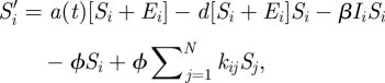
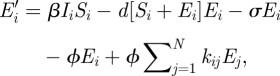
Our model follows a standard SEI (susceptible–exposed–infectious) compartment-based approach to disease modelling in which the host population is structured in terms of the infection status of individuals [23,24]. For raccoon rabies, the host population is divided into susceptible, exposed and infectious classes. No recovered class is included since there is no indication of recovery from rabies infection in wild raccoon populations [25,26]. To add spatial structure, we divide the host population into a one-dimensional array of 100, 1 km patches to form a metapopulation [17,27]. Within each patch the disease dynamics are governed by a system of ordinary differential equations (ODEs):

2.1

2.2

2.3

2.4

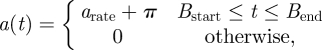
where N is the total number of locations and the spatial location is indexed by i and j (with i, j = 1 … N), and t represents time since the beginning of each year. At each location i, the density of susceptible, exposed and infectious individuals is represented by the state variables S_i, E_i and I_i, respectively. The per capita reproductive rate, a(t), is a periodic function and is applied to all subpopulations, i, resulting in synchronous reproduction over the entire metapopuation. In our model, we assume only non-infectious individuals are involved in reproduction (because of the short life expectancy and behavioural changes in rabies-infected raccoons) [26]. Newborn individuals are assumed to be susceptible.

The birth-pulse is implemented as a periodic step function:

2.5

where t is time measured in days since the beginning of each year (electronic supplementary material, figure S1). The total per capita number of births is held constant at 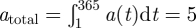kits per adult per year over the latitudinal gradient. As a consequence, the daily birth rate (a_rate) is a function of the birth-pulse width (B_width) and narrower northern birth-pulses have higher amplitudes than southern birth-pulses (electronic supplementary material, figure S1). The birth-pulse parameters B_start and B_end define the start and the end dates of the parturition period, respectively, and are adjusted based on the metapopulation's position along the north–south gradient to produce appropriate birth-pulse widths (B_width). Thus, for a birth-pulse width of B_width days and a mean birth date B_mean, B_start = B_mean − B_width/2, B_end = B_mean + B_width/2. We set the average birth date to be 5 May based on reported peaks in birth date for raccoons for all model results [20,28,29].

We introduce a simple white noise process into the model with the term π. The addition of the stochastic term to the birth-pulse function can be interpreted as the effects of random inter-annual variation in the environment that either increases or decreases the reproductive capacity of the host population. Following the approach taken by Rand & Wilson [30] and Ellner & Turchin [31] we allow the birth rate to vary from year to year by adding Gaussian-distributed noise to the reproduction term, where π is a random variable with a mean equal to zero, and a variance equal to 0.1a_total.

The addition of the white noise term addresses the often observed structural instability associated with the chaotic dynamics produced by the periodic forcing of ODEs. An analysis of the single-patch dynamics of our model (i.e. without a spatial dimension) without white noise (π = 0) reveals positive Lyaponov exponents over a substantial range of birth-pulses indicating the presence of chaotic dynamics (electronic supplementary material, figure S2b). Chaotic dynamics emerge in our model because the natural period of the system (0.904 years) is close to the 1 year period of external forcing and we expect chaotic dynamics to appear as a consequence of resonance effects [32]. Chaotic dynamics are present in other seasonally forced SIR (susceptible–infectious–recovered) models [10–12,14,33] and there is scepticism about the role chaos plays in the dynamics of natural populations [31]. In particular, models with chaotic dynamics exhibit a degree of structural instability such that adding environmental noise can profoundly change model dynamics [30]. We include the white noise process to ensure that our results are not a peculiarity associated with the emergence of chaotic dynamics over certain ranges of seasonal forcing.

We assume the disease-free host population size is regulated by density-dependent effects on the rate of mortality arising from intraspecific competition for limited food and habitat. We incorporate the effects of density-dependent mortality using a standard logistic term governed by the model parameter d. Density estimates for disease-free raccoon populations in urban areas range from 21.1 to 66.7 ind km⁻² (45.7 ind km⁻² [34], 21.1 km⁻² [35], 66.7 ind km⁻² [21], 35.7 ind km⁻² [36] and 28.2 ind km⁻² [20]) with an arithmetic mean of approximately 39 ind km⁻². We use this value as the per-patch disease-free carrying capacity for the model (K = a/d) and assume a constant daily birth rate (a = 5/365 = 0.0137 d⁻¹) to obtain 3.51 × 10⁻⁴animal⁻¹ d⁻¹ as an estimated value for d. With seasonal reproduction, numerical results show the disease-free dynamics converge on a limit cycle with a period of 1 year with average densities between 39.2 ind km⁻² and 39.5 ind km⁻² for birth-pulse widths from 72 to 330 days.

Exposed individuals become infectious after a mean latency period of 1/σ = 22 days [37], yielding a per capita latency rate (σ) of 0.045 d⁻¹. We use a mean life expectancy of infectious raccoons of 1/α = 12.5 days [26]. Given the other model parameters, our estimate for the transmission rate (β = 0.04) is chosen to give a basic reproduction rate (R₀) of 1.6, which is within the reported range for rabies [38].

We initiate epidemic dynamics in each simulation by introducing a single-infected individual into a host population at its disease-free limit cycle.

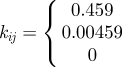
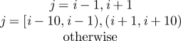
Host dispersal links patches within the metapopulation. The per capita rate of emigration is ϕ and the per capita rate of immigration to patch i, from all other patches, j, occurs at the rate ϕΣ_jk_ijS_j, where k_ij is the fraction of the emigrants from location j arriving in location i. A similar term in equation (2.2) describes the dispersal of exposed individuals. The model boundaries are reflecting and the overall population is closed with respect to dispersal. That is, the sum of the dispersing fractions from any location, j, to all other locations, i ≠ j, equals unity (i.e. Σ_i≠j k_ij = 1). For simplicity, we assume dispersal is symmetric and that individuals only move to immediate neighbours (i.e. k_j−1,j = k_j+1,j = 0.5, k_ij = 0 otherwise). The per capita emigration rate of infected individuals in equation (2.3) is given by ψ and the immigration rate into patch i is given by ψΣ_jk_ijI_j, where the k_ij's are the same as those used for the non-infectious classes. The immigration rate used in the model is ϕ = ψ = 0.025 d⁻¹. When combined with the dispersal coefficients (k_ij), the speed of the travelling wave of simulated infections is approximately 40 km yr⁻¹, consistent with reported rates of spread for rabies (38.4 ± 3.8 km yr⁻¹) [38,39]. All of the model parameters are summarized in table 1.

Table 1.

Model parameters, ‘baseline’ values and the parameter value variation used in the sensitivity analysis.

parameter	units	definition	‘baseline’ value	−15%	+15%
a(t)	day−1	birth-pulse function	—	—	—
atotal	yr−1	total annual per capita birth rate	5	4.25	5.75
Bmean	—	mean birth date	5 May	1 January	2 July
Bwidth	day	birth-pulse width	variable
Bstart	—	start of the parturition period	Bmean − Bwidth/2
Bend	—	end of the parturition period	Bmean + Bwidth/2
d	animal−1 d−1	density-dependant mortality rate	3.51 × 10−4	2.98 × 10−4	4.03 × 10−4
σ	d−1	latency rate	0.045	0.038	0.052
α	d−1	disease-induced mortality rate	0.08	0.068	0.092
ϕ	d−1	emigration rate for susceptible and exposed individuals	0.025	0.021	0.029
ψ	d−1	emigration rate for infected individuals	0.025	0.021	0.029
β	animal−1 d−1	transmission rate	0.04	0.034	0.046
kij	—	fraction of emigrants from j that move to i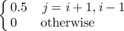

2.2. Measure of spatial synchronization

To measure the spatial synchronization of epidemics we compute the phase coherency [17] between the number of infectious individuals across locations (I_i, i = 1 … N). Phase coherency is a wavelet-based approach that computes the correlation between the phase angles of two time series [40]. We define a coherency function C(l) describing how phase coherency changes with l, the distance between patches. The coherency function is defined as the non-parametric cross-correlation function based on a smoothed spline fitted to the phase correlation between all unique pairs of patches using the R package ncf [41]. We computed the phase coherency function from our model results after first log-transforming the time series from each location and normalizing it to have zero mean and unit variance. To reveal the changes in spatial synchronization across a wide range of birth-pulse widths we distil the results of the phase coherency analysis to a single value characterizing the degree of synchronization. The degree of spatial synchronization produced under each birth-pulse is the distance, l*, at which the phase coherency C(l) is equal to the regional average correlation. Small values of l* indicate synchronization over short distances while large values indicate synchronization over longer distances. Additional details describing how we compute phase coherency are provided in the electronic supplementary material.

2.3. Model application at the regional scale

To investigate how spatial synchronization of epidemics within the metapopulation changes over the latitudinal gradient in seasonality we ran our model for birth-pulses from 72 to 330 days. This range of birth-pulse widths is based on reported parturition periods for northern and southern raccoon populations [20,28,29]. The degree of spatial synchronization at each birth-pulse width is computed as the average distance, , taken for 10 replicate runs. In each replicate, we computed l* from the last 10 years of a 20 year simulation. For all birth-pulse widths, the model entered into its long-term dynamic by the 10th year. Experiments with longer runs did not produce substantially different results.

3. Results

The rabies epidemic in a population experiencing the narrowest, northern, birth-pulse (72 days) forms a fragmented landscape of local outbreaks (figure 1a). In the first 3 years, infection spreads through the population in three waves corresponding to the seasonal addition of newly born individuals into the susceptible class. In subsequent years, seasonal reproduction does limit the timing of outbreaks, but within each year it does not synchronize population dynamics over space; instead it results in the creation of patches of asynchronous disease outbreak (figure 1a). The spatial asynchrony of outbreaks is reflected in a small value for the phase coherency, indicating that the correlation was only significant over a short distance ( = 5 km). The patchy distribution of epidemics that emerges under the shortest birth-pulse width (72 days) persists even though locally, individual patch dynamics converge on a limit cycle for every initial condition (see Lyapunov exponent less than zero in the electronic supplementary material, figure S2b). In contrast to the northern populations, the spatial dynamics at the southernmost end of the latitudinal gradient (B_width = 330 days) are highly synchronized during the endemic phase and result in large values for indicating substantial spatial synchronization over long distances (=40 km; figure 1b).

Figure 1.

(a) Asynchronous and (b) synchronous spatial dynamics produced under the strong (72 day) and weak (330 day) birth-pulse. In each figure, time (years) proceeds from left to right, space is shown along the axis moving into the figure and the height is the density of infectious raccoons. Colour is added to each plot for clarity and indicates the density of infectious individuals; a colour gradient from blue to red is used to indicate densities ranging from low to high.

Seasonally forced models can exhibit multiple attractors and both cyclic and chaotic dynamics may coexist over certain parameter ranges [11]. In such systems, the attractor that governs the long-term dynamics depends on the initial conditions. We analysed our model to explore the possible coexistence of chaotic and period attractors as an explanation for the patchy distribution of epidemics. Bifurcation diagrams computed from our model with 2, 3 or 4 patches show that model dynamics converge on periodic orbits (electronic supplementary material, figure S3). These figures indicate that for narrow birth-pulse widths, the long-term dynamics of our model are not influenced by chaotic dynamics. To evaluate the model behaviour during the initial stage of the epidemic we computed the direct finite-time Lyapunov exponents (DLEs) for the single-patch version of our model based on a 50 year simulation [42]. The DLEs are generally lower for short birth-pulse widths (electronic supplementary material, figure S4) indicating a short-term dynamics with lower sensitivity to initial conditions than for longer birth-pulse widths. Collectively, these results suggest that chaotic behaviours are not the drivers of the loss of synchronization when the length of the birth-pulse is short.

Results computed over the latitudinal gradient in birth-pulse widths indicate an overall trend towards increasing spatial synchronization from north to south (figure 2). The trend is divided into three ranges, with spatial synchronization increasing at different rates as the birth-pulse width is increased (figure 2). Over the first range, from 72 to 200 days, there is a modest increase in the degree of spatial synchronization. From 200 to 270 days, there is a slight decrease in spatial synchronization, followed by a rapid increase from = 12 km to =40 km for birth-pulse widths from 270 to 330 days.

Figure 2.

Pattern of increasing spatial synchronization () along the north–south latitudinal gradient in seasonality. The degree of spatial synchronization is averaged over 10 replicate runs of the model.

We performed a sensitivity analysis of our model to evaluate the robustness of the latitudinal gradient in spatial synchronization. We found the pattern of increasing spatial synchrony persists over a range of values for each model parameter and for changes in the initial conditions. For most parameters and initial conditions, we considered the effects of increasing or decreasing the value by 15 per cent relative to the ‘baseline’ values (table 1). As an additional test of the initial conditions, we examined the effects of initiating the infection at five different locations between the edge and the centre of the one-dimensional array (patches 10, 20, 30, 40 and 50). To test for sensitivity to the dispersal coefficients (k_ij) we added long-distance translocations (LDTs; electronic supplementary material, table S1). We also considered the effects of moving the mean birth date (B_mean) to different times of the year (1 January and 2 July), changing when the simulated epidemic was initiated relative to the annual peak in the number of susceptible hosts. Moving the mean birth date (B_mean) to 1 January synchronizes the start of the epidemic with the annual susceptible peak while a mean birth date of 2 July synchronizes the start of the epidemic with lowest number of susceptible individuals. The effects of changing the model parameters were evaluated relative to the baseline results (i.e. the results based on the baseline parameters in table 1).

The pattern of increasing spatial synchronization was most sensitive to changing the total birth rate (a_total), the rate at which latently infected individuals become infectious (σ), and the mean birth date (B_mean; figure 3). However, in each case the overall pattern of increasing spatial synchronization was still evident. We applied smoothing splines to clarify the sensitivity of our results to varying the model parameters. We also applied a 90% confidence interval (CI; computed for the spline fitted to the baseline results) to assess the sensitivity of the model. Varying a_total, σ and B_mean produced patterns of increasing spatial synchronization that fell outside the 90% CI. The effects of increasing the total birth rate (a_total) on the pattern of spatial synchronization were variable (figure 3a). Increasing a_total reduced spatial synchronization relative to the baseline results for birth-pulse widths from 72 to 150 days and 326 to 330 days, but spatial synchronization increased over intermediate pulse widths (150–326 days). The changes produced by decreasing a_total were smaller and fell within the 90% CI for most birth-pulse widths. Increasing the latency rate (σ) resulted in a decrease in spatial synchronization over all birth-pulse widths, while decreasing the latency rate increased the degree of spatial synchronization (figure 3b). The effects of increasing or decreasing σ were more pronounced as the birth-pulse width increased and fell outside the 90% CI for birth-pulses longer than 200 days. Moving B_mean to 1 January decreased spatial synchronization over all but the longest birth-pulse widths while a mean birth date of 2 July produced a pattern of spatial synchronization similar to the baseline results (figure 3c).

Figure 3.

Model sensitivity analysis showing the change in the relationship between spatial synchronization () and the birth-pulse width (B_width) for a 15% change in (a) the total birth rate (a_total), (b) the rate at which latently infected individuals become infectious (σ) and (c) the mean birth date of the birth-pulse (B_mean). In all panels, the results for the ‘baseline’ parameters (table 1) are plotted in black. In panels (a) and (b) the results of increasing the parameter value by 15% are plotted in blue and the results of decreasing the parameter by 15% are shown in red. In panel (c) the results of moving the mean birth date to 1 January or 2 July are plotted in red or blue, respectively. Each dot is the mean of 10 replicate runs. Lines are smooth splines fitted to the data using 7 d.f. and are included to clarify the changes in spatial synchronization produced by varying model parameters. The shaded region is a 90% confidence interval for the spline fitted to the baseline results (black line and dots) and is included to assess the sensitivity of the model results.

Our results were robust to changes in the rate of disease-induced mortality (α), the transmission rate (β), the rate of density-dependent mortality (d) and the dispersal rates (ϕ and ψ; electronic supplementary material, figure S5a–e). A 15 per cent increase or decrease in these parameters produced a relationship between spatial synchronization and birth-pulse widths that consistently fell within a 90% CI for the baseline results. Adding LDT to the dispersal processes also had a relatively small effect on the model results (electronic supplementary material, figure S5f). Model results were also robust to changing the initial conditions (electronic supplementary material, figure S6). Results from a 15 per cent increase or decrease in the initial density of susceptible individuals were similar to those for the baseline parameters (electronic supplementary material, figure S6a). Furthermore, changing where the epidemic started within the metapopulation had little effect on the pattern of increasing spatial synchronization (electronic supplementary material, figure S6b–f).

In our results we focus on the spatial dynamics over a 20 year time horizon. This period of time is comparable to the duration of the mid-Atlantic raccoon rabies epidemic that was initiated in 1977. However, we find that the pattern of increasing spatial synchronization shown in figure 2 persists for up to 200 years (electronic supplementary material, figure S7). These results suggest that the differences in spatial synchronization that emerge between northern and southern populations are a persistent feature of seasonally forced disease dynamics.

4. Discussion

Our results are the first to our knowledge to suggest a predictable geographical gradient in the spatial synchronization of epidemics. The latitudinal gradient in seasonally variable host demography may result in a gradient in epidemiological dynamics over which the local epidemics become progressively more spatially synchronized. A recent analysis of measles cases in sub-Saharan Africa convincingly illustrates the potential for strong seasonal forcing, produced in this case by the annual rainy season, to desynchronize measles dynamics in different departments (subregions) of Niger [43]. That analysis supports our theoretical results suggesting that strong periodic forcing can produce spatial asynchrony in disease dynamics. Here, we have shown that shifts in population dynamics associated with a gradient in host demography can result in a continuous gradient in the spatial synchronization of epidemics.

The effect of seasonality on the spatial synchronization of metapopulation dynamics has been addressed in a number of previous studies [10–17]. Lloyd & May [16] reported results from a seasonally forced metapopulation model in which local population dynamics switch from synchronized to desynchronized as chaotic dynamics emerge. Allen et al. [44] showed that chaotic dynamics decrease synchronization between patches, reducing the overall risk of global extension. Allen et al. [44] characterized the contribution of local dynamics to persistence measured at the level of the entire metapopulation but do not quantify the degree of spatial synchronization that emerges among locations.

The differences in the spatial structure of epidemics between northern and southern populations are the result of an interaction between the wave-like spread of infection and the length of the birth-pulse. The birth-pulse produces annual cycles in the disease-free dynamics at locations ahead of the epidemic. As a result, the epidemic wavefront encounters different densities of susceptible individuals as it sweeps through the metapopulation. At the northern end of the latitudinal gradient, the amplitude of the disease-free cycle is large and the epidemic wavefront encounters substantial differences in susceptible densities as it sweeps through the metapopulation. Numerical results from a non-spatial version of the model under the action of a narrow birth-pulse show different dynamics emerge when an epidemic is initialized at different phases of the host's reproductive cycle (electronic supplementary material, figure S8). In our spatial model, the differences between locations persist because of the relatively weak linkage associated with dispersal over long distances. In southern populations, the nearly constant birth-pulse results in relatively small oscillations in population size. As a result, the local disease dynamics are initiated under nearly identical conditions and small differences are eventually eliminated by dispersal.

The results of our study represent a new conclusion into the pattern of spatial synchronization of metapopulation dynamics. Here, we have shown that spatial synchronization can vary continuously over a gradient of seasonal forcing. Our results are qualitatively consistent with earlier results in which dynamics shift between synchronized and desynchronized populations under different levels of seasonal forcing [16]. Our results suggest that the effects of seasonal forcing are not limited to one of two outcomes, and may lead to a range of different results that vary continuously with variations in the strength of seasonal forcing. This conclusion can have important consequences and implications for the design of infectious disease control strategies.

The surveillance of existing and emergent infectious diseases in wildlife is an integral part of public health planning [45]. Wildlife populations are reservoirs for diseases that infect humans, and recent estimates suggest that the majority of emergence events arise from wildlife populations [46]. At the same time that researchers have become more aware of the importance of monitoring and controlling epidemics in wildlife, public health funding is dwindling [45]. This necessitates a targeted approach to monitoring populations at risk to make the best use of limited resources.

Our results suggest that underlying demographic variations in the host populations may influence the design of optimal surveillance strategies. In areas where host population demographic parameters are characterized by little or no seasonal variation, the samples taken at a few locations can reasonably be used as a proxy for an entire region. Public health resources can be saved by restricting monitoring and control efforts in these areas. In areas where host demographics are strongly seasonal, a substantially larger surveillance programme may be required to obtain a reasonable estimate of outbreak intensity over the entire region.

Our conclusions are based on our simulation of the raccoon-rabies dynamics of the mid-Atlantic regions of the USA. However, the modelling framework is general and the results are robust to changes in the model parameters and initial conditions. These factors suggest our model results may be applicable to other zoonotic diseases with important public health consequences and as well as human infections. A number of wildlife species in North America have been struck by rabies epidemics including skunk (Mephitis mephitis) and fox (Vulpis vulpis) populations [26]. Both species have a distinct reproductive season and an extensive latitudinal range [47,48]. Rabies epidemics in skunks also exhibit pronounced seasonal cycles in the prevalence of rabies infection [49]. As an example of a non-zoonotic human disease, recent analysis of measles dynamics in Africa suggests that spatial asynchrony in prevalence may arise from seasonal increase in contact between people associated with an increase in indoor activities during the rainy season [43].

The model produces hypotheses that are directly testable using time-series data that are spatial explicit and recorded at high spatial resolution. These data are not available. We are working closely with the US Centers for Disease Control and Prevention (CDC), the US Department of Agriculture and state public health offices to collect data that are appropriate to test these hypotheses. This new source of data is necessary for testing the results of our model. The existing rabies database, coordinated by the CDC, while extensive, does not provide the spatial resolution required to test our model. The spatial resolution of the CDC database is not consistent across the eastern USA, ranging from townships (mean = 93 km²) in some northern states (e.g. Connecticut) to counties (mean = 1600 km²) in other states (e.g. Georgia). Both of these geographical units are much larger than the scale at which patterns emerge within our model (patch = 1 × 1 km²).

Seasonality is becoming recognized as an increasingly important component in understanding infectious disease [1,50,51]. However, few studies recognize the significance of geographical variation in the structure of the seasonal signal on widely distributed infectious diseases. Widely distributed pandemic diseases pose a substantial public health threat and we need accurate models to guide surveillance and control policies. Results from our model indicate that geographical gradients in demographic structure may produce associated gradients in the spatial synchronization of epidemics. Including these forms of geographical variation is critical for increasing the predictive power and utility of infectious disease models used for public health surveillance and control.

References

- 1.Altizer S., Dobson A., Hosseini P., Hudson P., Pascual M., Rohani P. 2006. Seasonality and the dynamics of infectious diseases. Ecol. Lett. 9, 467–484 10.1111/j.1461-0248.2005.00879.x (doi:10.1111/j.1461-0248.2005.00879.x) [DOI] [PubMed] [Google Scholar]
- 2.Fisman D. N. 2007. Seasonality of infectious diseases. Annu. Rev. Public Health 28, 127–143 10.1146/annurev.publhealth.28.021406.144128 (doi:10.1146/annurev.publhealth.28.021406.144128) [DOI] [PubMed] [Google Scholar]
- 3.Dowell S. F. 2001. Seasonal variation in host susceptibility and cycles of certain infectious diseases. Emerg. Infect. Dis. 7, 369–374 [DOI] [PMC free article] [PubMed] [Google Scholar]
- 4.Sonenshine D. E., Mather T. N. (eds) 1994. Ecological dynamics of tick-borne zoonoses. Oxford, UK: Oxford University Press [Google Scholar]
- 5.Hosseini P. R., Dhondt A. A., Dobson A. 2004. Seasonality and wildlife disease: how seasonal birth, aggregation and variation in immunity affect the dynamics of Mycoplasma gallisepticum in house finches. Proc. R. Soc. Lond. B 271, 2569–2577 10.1098/rspb.2004.2938 (doi:10.1098/rspb.2004.2938) [DOI] [PMC free article] [PubMed] [Google Scholar]
- 6.Pascual M., Bouma M. J., Dobson A. P. 2002. Cholera and climate: revisiting the quantitative evidence. Microbes Infect. 4, 237–245 10.1016/S1286-4579(01)01533-7 (doi:10.1016/S1286-4579(01)01533-7) [DOI] [PubMed] [Google Scholar]
- 7.Simonsen L. 1999. The global impact of influenza on morbidity and mortality. Vaccine 17, S3–S10 10.1016/S0264-410X(99)00099-7 (doi:10.1016/S0264-410X(99)00099-7) [DOI] [PubMed] [Google Scholar]
- 8.Cook S. M., Glass R. I., Lebaron C. W., Ho M. S. 1990. Global seasonality of rotavirus infections. Bull. World Health Organ. 68, 171–177 [PMC free article] [PubMed] [Google Scholar]
- 9.Altizer S., Hochachka W. M., Dhondt A. A. 2004. Seasonal dynamics of mycoplasmal conjunctivitis in eastern North American house finches. J. Anim. Ecol. 73, 309–322 10.1111/j.0021-8790.2004.00807.x (doi:10.1111/j.0021-8790.2004.00807.x) [DOI] [Google Scholar]
- 10.Bolker B. M., Grenfell B. T. 1993. Chaos and biological complexity in measles dynamics. Proc. R. Soc. Lond. B 251, 75–81 10.1098/rspb.1993.0011 (doi:10.1098/rspb.1993.0011) [DOI] [PubMed] [Google Scholar]
- 11.Earn D. J., Rohani P., Bolker B. M., Grenfell B. T. 2000. A simple model for complex dynamical transitions in epidemics. Science 287, 667–670 10.1126/science.287.5453.667 (doi:10.1126/science.287.5453.667) [DOI] [PubMed] [Google Scholar]
- 12.Grenfell B. T. 1992. Chance and chaos in measles dynamics. J. R. Stat. Soc. B 54, 383–398 [Google Scholar]
- 13.Grenfell B. T., Bolker B. M. 1998. Cities and villages: infection hierarchies in a measles metapopulaiton. Ecol. Lett. 1, 63–70 10.1046/j.1461-0248.1998.00016.x (doi:10.1046/j.1461-0248.1998.00016.x) [DOI] [Google Scholar]
- 14.Grenfell B. T., Bolker B. M., Kleczkowski A. 1995. Seasonality and extinction in chaotic metapopulations. Proc. R. Soc. Lond. B 259, 97–103 10.1098/rspb.1995.0015 (doi:10.1098/rspb.1995.0015) [DOI] [Google Scholar]
- 15.Keeling M. J., Grenfell B. T. 1997. Disease extinction and community size: modeling the persistence of measles. Science 275, 65–67 10.1126/science.275.5296.65 (doi:10.1126/science.275.5296.65) [DOI] [PubMed] [Google Scholar]
- 16.Lloyd A. L., May R. M. 1996. Spatial heterogeneity in epidemic models. J. Theor. Biol. 179, 1–11 10.1006/jtbi.1996.0042 (doi:10.1006/jtbi.1996.0042) [DOI] [PubMed] [Google Scholar]
- 17.Grenfell B. T., Bjornstad O. N., Kappey J. 2001. Travelling waves and spatial hierarchies in measles epidemics. Nature 414, 716–723 10.1038/414716a (doi:10.1038/414716a) [DOI] [PubMed] [Google Scholar]
- 18.Feldhamer G. A., Chapman J. A., Thompson B. C. (eds) 2003. Wild mammals of North America. Baltimore, MD: Johns Hopkins University Press [Google Scholar]
- 19.Rohani P., Earn D. J. D., Grenfell B. T. 1999. Opposite patterns of synchrony in sympatric disease metapopulations. Science 286, 968–971 10.1126/science.286.5441.968 (doi:10.1126/science.286.5441.968) [DOI] [PubMed] [Google Scholar]
- 20.Gehrt S. D. 2003. Raccoons and allies. In Wild mammals of North America (eds Feldhamer G. A., Chapman J. A., Thompson B. C.), 2nd edn. Baltimore, MD: John Hopkins University Press [Google Scholar]
- 21.Hoffmann C. O., Gottschang J. L. 1977. Numbers, distribution, and movements of a raccoon population in a suburban residential community. J. Mammal. 58, 623–636 10.2307/1380010 (doi:10.2307/1380010) [DOI] [Google Scholar]
- 22.Riley S. P. D., Hadidian J., Manski D. A. 1998. Population density, survival, and rabies in raccoons in an urban national park. Can. J. Zool. 76, 1153–1164 10.1139/cjz-76-6-1153 (doi:10.1139/cjz-76-6-1153) [DOI] [Google Scholar]
- 23.Anderson R. M., May R. M. 1991. Infectious diseases of humans: dynamics and control. Oxford, UK: Oxford University Press [Google Scholar]
- 24.Kermack W. O., Mckendrick A. G. 1927. Contributions to the mathematical theory of epidemics. Proc. R. Soc. Lond. A 115, 700–721 10.1098/rspa.1927.0118 (doi:10.1098/rspa.1927.0118) [DOI] [Google Scholar]
- 25.Childs J. E., Curns A. T., Dey M. E., Real L. A., Feinstein L., Bjornstad O. N., Krebs J. W. 2000. Predicting the local dynamics of epizootic rabies among raccoons in the United States. Proc. Natl Acad. Sci. USA 97, 13 666–13 671 10.1073/pnas.240326697 (doi:10.1073/pnas.240326697) [DOI] [PMC free article] [PubMed] [Google Scholar]
- 26.Jackson A. C., Wunner W. (eds) 2007. Rabies. New York, NY: Academic Press [Google Scholar]
- 27.Tompkins D. M., White A. R., Boots M. 2003. Ecological replacement of native red squirrels by invasive greys driven by disease. Ecol. Lett. 6, 189–196 10.1046/j.1461-0248.2003.00417.x (doi:10.1046/j.1461-0248.2003.00417.x) [DOI] [Google Scholar]
- 28.Johnson A. S. 1970. Biology of the raccoon in Alabama. Bulletin 402, Alabama Agricultural Experiment Station, Auburn University, USA [Google Scholar]
- 29.Stuewer F. W. 1943. Raccoons: their habits and management in Michigan. Ecol. Monogr. 13, 203–257 10.2307/1943528 (doi:10.2307/1943528) [DOI] [Google Scholar]
- 30.Rand D. A., Wilson H. B. 1991. Chaotic stochasticity—a ubiquitous source of unpredictability in epidemics. Proc. R. Soc. Lond. B 246, 179–184 10.1098/rspb.1991.0142 (doi:10.1098/rspb.1991.0142) [DOI] [PubMed] [Google Scholar]
- 31.Ellner S., Turchin P. 1995. Chaos in a noisy world—new methods and evidence from time-series analysis. Am. Nat. 145, 343–375 10.1086/285744 (doi:10.1086/285744) [DOI] [Google Scholar]
- 32.Greenman J., Kamo M., Boots M. 2004. External forcing of ecological and epidemiological systems: a resonance approach. Physica D 190, 136–151 10.1016/j.physd.2003.08.008 (doi:10.1016/j.physd.2003.08.008) [DOI] [Google Scholar]
- 33.Bolker B. 1993. Chaos and complexity in measles models—a comparative numerical study. IMA J. Math. Appl. Med. Biol. 10, 83–95 10.1093/imammb/10.2.83 (doi:10.1093/imammb/10.2.83) [DOI] [PubMed] [Google Scholar]
- 34.Williams A. B. 1936. The composition and dynamics of a beech-maple climax community. Ecol. Monogr. 6, 317–408 10.2307/1943219 (doi:10.2307/1943219) [DOI] [Google Scholar]
- 35.Butterfield R. T. 1944. Populations, hunting pressure, and movement of Ohio raccoons. Trans. N. Am. Wildl. Nat. Resour. Conf. 9, 337–344 [Google Scholar]
- 36.Jacobsen J. E. 1982. Parasite relationships between an urban and a rural raccoon population. In Ecology. West Lafayette, IN: Purdue University [Google Scholar]
- 37.Bigler W. J., Mclean R. G., Trevino H. A. 1973. Epizootiologic aspects of raccoon rabies in Florida. Am. J. Epidemiol. 98, 326–335 [DOI] [PubMed] [Google Scholar]
- 38.Biek R., Henderson J. C., Waller L., Rupprecht C. E., Real L. A. 2007. A high-resolution genetic signature of demographic and spatial expansion in epizootic rabies virus. Proc. Natl Acad. Sci. USA 104, 7993–7998 10.1073/pnas.0700741104 (doi:10.1073/pnas.0700741104) [DOI] [PMC free article] [PubMed] [Google Scholar]
- 39.Childs J. E., Real L. A. 2007. Epidemiology. In Rabies (eds Jackson A. C., Wunner W. H.), 2nd edn. New York, NY: Elsevier [Google Scholar]
- 40.Torrence C., Compo G. P. 1998. A practical guide to wavelet analysis. Bull. Am. Meteorol. Soc. 79, 61–78 (doi:10.1175/1520-0477(1998)079<0061:APGTWA>2.0.CO;2) [DOI] [Google Scholar]
- 41.Bjornstad O. N. 2009. Ncf: spatial nonparametric covariance functions. R package version 1.1–3. See http://onb.Ent.Psu.Edu/onb1/r
- 42.Aldridge B. B., Haller G., Sorger P. K., Lauggenburger D. A. 2006. Direct Lyapunov exponent analysis enables parametric study of transient signalling cell behaviour. IEE Proc. Syst. Biol. 153, 425–432 10.1049/ip-syb:20050065 (doi:10.1049/ip-syb:20050065) [DOI] [PubMed] [Google Scholar]
- 43.Ferrari M. J., Grais R. F., Bharti N., Conlan A. J. K., Bjornstad O. N., Wolfson L. J., Guerin P. J., Djibo A., Grenfell B. T. 2008. The dynamics of measles in sub-Saharan Africa. Nature 451, 679–684 10.1038/nature06509 (doi:10.1038/nature06509) [DOI] [PubMed] [Google Scholar]
- 44.Allen J. C., Schaffer W. M., Rosko D. 1993. Chaos reduces species extinction by amplifying local-population noise. Nature 364, 229–232 10.1038/364229a0 (doi:10.1038/364229a0) [DOI] [PubMed] [Google Scholar]
- 45.Stark K. D. C., Regula G., Hernandez J., Knopf L., Fuchs K., Morris R. S., Davies P. 2006. Concepts for risk-based surveillance in the field of veterinary medicine and veterinary public health: review of current approaches. BMC Health Serv. Res. 6, 1–8 10.1186/1472-6963-6-20 (doi:10.1186/1472-6963-6-20) [DOI] [PMC free article] [PubMed] [Google Scholar]
- 46.Jones K. E., Patel N. G., Levy M. A., Storeygard A., Balk D., Gittleman J. L., Daszak P. 2008. Global trends in emerging infectious diseases. Nature 451, 990–994 10.1038/nature06536 (doi:10.1038/nature06536) [DOI] [PMC free article] [PubMed] [Google Scholar]
- 47.Godin A. J. 1982. Striped and hooded skunks. In Wild mammals of North America (ed. Feldhamer G. A.). Baltimore, MD: Johns Hopkins University Press [Google Scholar]
- 48.Samuel D. E., Nelson B. B. 1982. Foxes. In Wild mammals of North America (eds Chapman J. A., Feldhamer G. A.). Baltimore, MD: Johns Hopkins University Press [Google Scholar]
- 49.Gramillion-Smith C., Woolf A. 1988. Epizootiology of skunk rabies in North America. J. Wildl. Dis. 24, 620–626 [DOI] [PubMed] [Google Scholar]
- 50.Fine P. E., Clarkson J. A. 1982. Measles in England and Wales—I. An analysis of factors underlying seasonal patterns. Int. J. Epidemiol. 11, 5–14 10.1093/ije/11.1.5 (doi:10.1093/ije/11.1.5) [DOI] [PubMed] [Google Scholar]
- 51.Schaffer W. M., Kot M. 1985. Nearly one dimensional dynamics in an epidemic. J. Theor. Biol. 112, 403–427 10.1016/S0022-5193(85)80294-0 (doi:10.1016/S0022-5193(85)80294-0) [DOI] [PubMed] [Google Scholar]