Multiple-rule bias in the comparison of classification rules

Abstract

Motivation: There is growing discussion in the bioinformatics community concerning overoptimism of reported results. Two approaches contributing to overoptimism in classification are (i) the reporting of results on datasets for which a proposed classification rule performs well and (ii) the comparison of multiple classification rules on a single dataset that purports to show the advantage of a certain rule.

Results: This article provides a careful probabilistic analysis of the second issue and the ‘multiple-rule bias’, resulting from choosing a classification rule having minimum estimated error on the dataset. It quantifies this bias corresponding to estimating the expected true error of the classification rule possessing minimum estimated error and it characterizes the bias from estimating the true comparative advantage of the chosen classification rule relative to the others by the estimated comparative advantage on the dataset. The analysis is applied to both synthetic and real data using a number of classification rules and error estimators.

Availability: We have implemented in C code the synthetic data distribution model, classification rules, feature selection routines and error estimation methods. The code for multiple-rule analysis is implemented in MATLAB. The source code is available at http://gsp.tamu.edu/Publications/supplementary/yousefi11a/. Supplementary simulation results are also included.

Contact: edward@ece.tamu.edu

Supplementary Information: Supplementary data are available at Bioinformatics online.

1 INTRODUCTION

Three recent articles in Bioiformatics have lamented the difficulty in establishing performance advantages for proposed classification rules (Boulesteix, 2010; Jelizarow et al., 2010; Rocke et al., 2009). Two statistically grounded sources of overoptimism have been highlighted. One considers applying a classification rule to numerous datasets and then reporting only the results on the dataset for which the designed classifier possesses the lowest estimated error. The optimistic bias from this kind of dataset picking is quantitatively analyzed in Yousefi et al. (2010), where it is termed ‘reporting bias’ and where this bias is characterized as a function of the number of considered datasets. A second kind of overoptimism concerns the comparison of a collection of classification rules by applying the classification rules to a dataset and comparing them according to the estimated errors of the designed classifiers. This kind of bias, which we will call ‘multiple-rule bias’, has been considered in Boulesteix and Strobl (2009) by applying a battery of classification rules to colon cancer and prostate cancer datasets and then examining the effects of choosing classification rules having minimum cross-validation error estimates.

Whereas the thrust of Boulesteix and Strobl (2009) is to compare the sources of multiple-rule bias in classification rules, namely, gene selection, parameter selection and classifier function construction, our interest is in studying multiple-rule bias as a function of the number of rules being considered. In particular, we are interested in the joint distribution, as a function of the number of compared rules, between the minimum estimated error among a collection of classification rules and the true error for the classification rule having minimum estimated error, as well as certain moments associated with this joint distribution. Although different with regard to distributional specifics, this approach is analogous to the approach taken in Yousefi et al. (2010), where the joint distribution involved the minimum estimated error of the designed classifier over a collection of datasets and the true error of the designed classifier on the population corresponding to the dataset resulting in minimum estimated error. This is a natural way to proceed because any bias ultimately results from inaccuracy in error estimation, so that the behavior of the joint distribution of interest and its moments are consequent to the joint distribution of the error estimator and the true error. Owing to the methodology in Boulesteix and Strobl (2009), it would have been impossible for them to study this joint distribution because they never concern themselves with true errors, only cross-validation estimates. Hence, when they compare a minimal error to a baseline error to arrive at a measure of optimistic bias, they are comparing cross-validation estimates.

In characterizing multiple-rule bias, we begin with a more general framework than the one just described; rather than simply considering multiple classification rules, we consider multiple classifier rule models, so that there are not only multiple classification rules, but also multiple error estimation rules being employed. We define a classifier rule model as a pair (Ψ, Ξ), where Ψ is a classification rule, including feature selection if feature selection is employed, and Ξ is an error estimation rule (Dougherty and Braga-Neto, 2006). The scenario in the preceding paragraph results where there is only a single error estimation rule.

2 SYSTEMS AND METHODS

We consider r classification rules, Ψ ₁, Ψ ₂, … , Ψ _r, and s error estimation rules, Ξ ₁, Ξ ₂, … , Ξ _s, on a feature-label distribution F. These are combined to form m = rs classifier rule models: (Ψ ₁, Ξ ₁), (Ψ ₁, Ξ ₂), … , (Ψ₁, Ξ _s), (Ψ ₂, Ξ ₁), (Ψ ₂, Ξ ₂), … , (Ψ _r, Ξ_s). Given a random sample _n of size n drawn from F, the classification rules yield r designed classifiers: Ψ _i = Ψ _i(_n), i = 1, 2, … , r. The true error of ψ _i is given by ϵ _trueⁱ = P(ψ _i(X) ≠ Y), where (X, Y) is a feature-label pair. For j = 1, 2, … , s, Ξ _j provides an error estimate, ϵ _est^{i, j}, for ψ _i. Since the classification rules are not identical, neither are the distributions of ϵ _true¹, ϵ _true², … , ϵ _true^r nor are the distributions of ϵ _est^{i, 1}, ϵ _est^{i, 2}, … , ϵ _est^{i, s}. All true-error and estimated-error distributions are functions of the random sample _n. Since all classification rules operate on the same sample, the true errors can be highly correlated, as will be the estimated errors. Without loss of generality, we assume the classifier models are enumerated so that E_n[ ϵ _true¹] ≤ E_n[ ϵ _true²] ≤ … ≤ E_n[ ϵ _true^r].

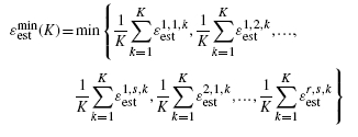
The minimum estimated error is

(1)

Letting i_min and j_min denote the classifier number and error estimator number, respectively, for which the error estimate is minimum, we have ϵ _est^min = ϵ _est^{i_min, j_min}.

Suppose a researcher wishes to select the best performing of r classification rules on a feature-label distribution F and proceeds by taking a random sample from F, designing a classifier for each classification rule, and estimating the errors of the designed classifiers. If F is known, then the true error of each designed classifier can be evaluated, the classifier with minimum true error can be chosen, and the classification rule leading to that classifier be declared ‘ best’. The truly best classification rule has the minimum expected error across all samples from F, so that what is happening is that a single observation of ϵ _trueⁱ is being used as an estimate for E_n[ϵ _trueⁱ]. On the other hand, if F is unknown as is used in practice, then the errors of the designed classifiers are estimated from sample data and the classification rule leading to the classifier, ψ _imin, with minimum estimated error is chosen as ‘best’. We are assuming that the researcher tries s error estimators and selects the one with lowest error estimate. In this case, a single observation of ϵ _est^min is being used to estimate E_n[ϵ _true^i_min], the basic performance measure for Ψ _imin. At issue is the goodness of this estimation. This involves the distribution of the deviation Δ = ϵ _est^min − E_n[ϵ _est^i_min], which is marginal to the joint distribution of (ϵ _est^min, ϵ _est^i_min).

A key performance measure derived from the deviation distribution is the bias of ϵ _est^min as an estimator of E_n[ϵ _true^i_min], namely,

(2)

Estimation is optimistic if Bias(m, n) < 0. This can happen even if none of the error estimation rules are optimistically biased, that is, even if E_n[ϵ _est^{i, j}] ≥ E_n[ ϵ _estⁱ] for i = 1, 2, … , r and j = 1, 2, … , s. Indeed, even if this is so, owing to estimation-rule variance, on any given sample it may be that ϵ _est^min < ϵ _est¹. For instance, if among Ξ ₁, Ξ ₂, … , Ξ _s there is an error estimation rule, such as leave-one-out cross-validation, that is slightly (pessimistically) biased and possesses large variance, then we should expect that E_n[ ϵ _est^min] < E_n[ ϵ _est¹]. In this case, E_n[ ϵ _est^min] < E_n[ ϵ _est¹] ≤ E_n[ϵ _est^i_min] and Bias(m, n) < 0. In the way we have set up the general problem, not only can optimistic bias result from considering multiple estimated errors among classifiers but also from applying multiple error estimates for each classifier.

From the generic arguments made thus far, we can state two properties concerning the bias. First, as the number m of classifier models grows, the minimum of Equation (1) is taken over more estimated errors, thereby increasing ϵ _true¹ − ϵ _true^min and | Bias(m, n)| = E_n[ϵ _Bias^i_min] − E_n[ ϵ _Bias^Bias]. Second, as the sample size n is increased, under the typical condition that the variance of the error estimator decreases with increasing sample size, E_n[ ϵ _est^min] increases and | Bias(m, n)| decreases.

Bias is only one factor in estimating E_n[ϵ _true^i_min] by ϵ _est^min. Another is the variance of ϵ _est^min. In fact, one should consider the root-mean-square (RMS) error for ϵ _est^min as an estimator of E_n[ϵ _true^i_min], which is given by

(3)

Even should the bias be small, the estimation will not be accurate if the deviation variance is large.

As discussed thus far, the classification rules are fixed; however, since our interest is in the number of classification rules (and error estimators), not any particular rule or estimator, we assume there is a total of R classification rules from which we randomly choose r. This corresponds to a situation where a researcher selects r from among a large collection (R) of potential classification rules and applies s error estimators to each selected rule. Given r, there are possible collections of classification rules to be combined with s error estimators to form possible collections of classifier rule models of size m. Hence, the number m of classifier rule models increments according to s, 2s, … , Rs. We denote the collection of classifier models of size m by Φ _m. To get the distribution of errors, one needs to generate independent samples from the same feature-label distribution and apply the procedure shown in Figure 1.

Fig. 1.

Multiple-rule testing procedure on a single sample.

The previously discussed performance measures must be adjusted to take model randomization into account. Given a sample _n, for a realization of Φ _m we find an expected deviation according to Equation (2), but now we have a random process generating the realizations so we have to take the expectation over that process to obtain the expected bias,

(4)

where the subscript indicates the average over Φ _m. A similar averaging arises with the deviation variance to yield Var_Var(m, n) = E_Φm[Var_n[Δ |Φ _m]]. The RMS now takes the form

(5)

Having discussed the performance measures relating to estimating E_n[ϵ _true^i_min] by ϵ _est^min, we now consider the comparative advantage of the classification rule Ψ _imin. Its true comparative advantage with respect to the other considered classification rules is

(6)

Its estimated comparative advantage is given by

(7)

where we use the error estimator associated with the pair (i_min, j_min) for which the minimum estimated error is obtained (assuming that this would be the error estimator chosen by a researcher for the sake of consistency). The expectation, E_n[A_est], of this distribution gives the mean estimated comparative advantage of Ψ _imin with respect to the collection. A key bias to be considered is C_bias = E_n[A_bias] − A_bias because it measures over optimism in comparative performance. In the case of randomization, the true comparative advantage becomes E_Φm[A_true|Φ _m] and the mean estimated comparative advantage becomes E_Φm[E_n[A_est|Φ _m]].

2.1 Simulation design

We use a general model based on multivariate Gaussian distributions with a blocked covariance structure that conforms to various observations made in microarray expression-based studies (Hua et al., 2009). A battery of distribution models can be constructed by changing model parameters to generate different synthetic data samples. We also consider four real datasets.

2.1.1 Synthetic data

In microarray studies, assuming a blocked covariance matrix is a way of modeling groups of interacting genes where there is negligible interaction between the groups. It has been used in genomic classification to model genes collected into distinct pathways, each pathway being represented by a block (Dougherty et al., 2007; Shmulevich and Dougherty, 2007). As explained in Hua et al. (2009), although the model does not embrace all details of the experimental procedures, it is general enough to include major aspects and various complexity levels suitable for simulation of real-world scenarios. Sample points are taken from two equally likely classes, C₀ and C₁, having D features. Furthermore, by putting c equally likely subclasses in C₁, each having its own distribution, one can model cases like different stages or subtypes of a cancer. Each sample point in C₁ belongs to one and only one of these subclasses.

Features are categorized into two major groups, markers and non-markers. Markers resemble genes causing disease or susceptibility to disease. The groups have different class-conditional distributions for the two classes. They can be further categorized into two different types: global and heterogeneous markers. Global markers are homogeneously distributed among the two classes with D_gm-dimensional Gaussian distributions and parameters (μ ₀^gm, Σ ₀^gm) for class 0 and (μ ₁^gm, Σ ₁^gm) for class 1, where D_gm is the total number of global markers. Heterogeneous markers are divided into c subclasses within class 1. Each subclass is associated with D_hm mutually exclusive heterogeneous markers having D_hm-dimensional Gaussian distributions with parameters (μ ₁^hm, Σ ₁^hm). The sample points not belonging to this particular subclass are considered to have D_hm-dimensional Gaussian class-conditional distributions with parameters (μ₀^hm, Σ ₀^hm).

Assuming that global and heterogeneous markers possess identical covariance structures, we use {Σ ₀, Σ ₁} instead of {Σ ₀^gm, Σ ₁^gm} and {Σ ₀^hm, Σ ₁^hm}. We assume that Σ ₀ = σ ₀²Σ and Σ ₁ = σ ₁²Σ, where σ ₀² and σ ₁² can be different, and that Σ has the following block structure:

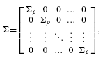where Σ _ρ is a l× l matrix, with 1 on the diagonal and ρ off the diagonal. In the block-based covariance structure, the markers are divided into equal-size blocks of size l. Markers of different blocks are uncorrelated, while all the markers in the same block are correlated to each other with correlation coefficient ρ.

A consequence of having unequal variances and subclasses in the class-conditional distributions is to introduce non-linearities in the decision boundaries for the model, where less global markers and larger difference in the variances lead to a more non-linear decision boundary. Because the global markers and the heterogeneous markers possess the same structure, we can assume the same mean vectors {μ ₀, μ ₁} for both groups, {μ ₀^gm, μ ₁^gm} and {μ ₀^hm, μ ₁^hm}, as we did for the covariance matrices. Furthermore, we use the same structure for μ ₀ and μ ₁ in the form of m₀× (1, 1, … , 1) and m₁× (1, 1, … , 1), respectively, where m₀ and m₁ are scalars (Hua et al., 2009; Yousefi et al., 2010).

Similar to the global markers, there are two types of non-markers: high-variance and low-variance non-markers. The D_hv features belonging to the former group are uncorrelated and their distributions are described by pN(m₀, σ ₀²)+(1 − p)N(m₁, σ ₁²), where m₀, m₁, σ ₀² and σ ₁² take values equal to the means and variances of the markers, respectively, and p is a random value uniformly distributed over [0, 1]. The D_lv remaining features are uncorrelated low-variance non-markers, each having a Gaussian distribution with parameters (m₀, σ ₀²).

A typical microarray experiment usually contains tens of thousands of probes (genes) but a small number of sample points, typically less than 200. We choose the total number of features to be D = 20000 and the number of sample points to be 60 and 120. Two variance settings are considered: equal variances {σ ₀² = 0.6², σ ₁² = 0.6²} and unequal variances {σ ₀² = 0.6², σ ₁² = 1.2²}. For the blocked covariance matrix, we choose block size l = 5 and correlation coefficient ρ = 0.8, giving relatively tight correlation within a block, which would be expected for a pathway. We do not choose model parameters in accordance with the Bayes errors or the estimated errors; rather, we choose them in accordance with achievable true errors seen in real problems. Table 1 shows the parameters of the distribution models used in this study. See Yousefi et al. (2010) for more details about the choice of parameters.

Table 1.

Distribution model parameters

Parameters	Values/description
Mean	m0= 0.23, m1= 0.8 (equal variance)
	m0= 0.11, m1= 0.9 (unequal variance)
Variances	σ20= 0.62, σ21= 0.62 (equal variance)
	σ20= 0.62, σ21= 1.22 (unequal variance)
Block size	l = 5
Features	D = 20000
Feature block correlation	ρ = 0.8
Subclasses	c = 2
Global markers	Dgm= 20
Heterogeneous markers	Dhm= 50
High-variance non-markers	Dhv= 2000
Low-variance non-markers	Dlv= 17 880

2.1.2 Real data

This study uses four real datasets from microarray experiments consisting of more than 150 arrays: pediatric acute lymphoblastic leukemia (ALL) (Yeoh et al., 2002), multiple myeloma (Zhan et al., 2006), hepatocellular carcinoma (HCC) (Chen et al., 2004) and drugs and toxicants response on rats dataset (Natsoulis et al., 2005). We use n = 60 sample points for training. The remaining sample points are held-out for computing the true error. To the extent possible, we try to maintain the original labeling and follow the data preparation directions used in the papers reporting these datasets. Table 2 shows a summary of the four real datasets. Full descriptions are presented in the Supplementary Materials.

Table 2.

A summary of the real datasets used in this study

Dataset	Dataset type	Feature|sample size
Yeoh et al. (2002)	Pediatric ALL	5077|149/99
Zhan et al. (2006)	Multiple myeloma	54 613|156/78
Chen et al. (2004)	HCC	10 237|75/82
Natsoulis et al. (2005)	Drugs response on rats	8491|120/61

2.2 Classification schemes

Six classification rules are considered: 3-nearest neighbors (3NN), linear discriminant analysis (LDA), diagonal LDA (DLDA), nearest-mean classifier (NMC), linear support vector machine (L-SVM) and radial basis function SVM (RBF-SVM). Two different feature selection methods are considered: t-test and t-test followed by sequential forward search (t-test + SFS). One-stage feature selection uses the t-test and five features are selected. For two-stage feature selection, the number of features is reduced to 500 in the first stage (t-test) and then to 5 by SFS. Three cross-validation error estimation methods are considered: 5-fold, 10-fold and leave-one-out (LOO). Combining six classification rules with two feature selection methods results in R = 12 classification rules from which we randomly choose r = 1, 2, … , R and design the classifiers on one sample. Note that with three error estimators, there is a maximum of 36 different classifier rule models. Table 3 lists the classification rules, feature selection methods and error estimation procedures utilized.

Table 3.

Classifier rule models considered in this study

Classification rule	Feature selection	Error estimation
3NN	t-test	5-fold cross-validation
LDA	t-test + SFS	10-fold cross-validation
DLDA		LOO
NMC
L-SVM
RBF-SVM

To illustrate the definitions, let us suppose we are only considering two classification rules, LDA and 3NN, without feature selection and two error estimators, LOO and CV5 (5-fold cross-validation). LDA is based on the discriminant for the optimal classifier in a Gaussian model (Gaussian class-conditional densities) with common covariance matrix by plugging the sample means and pooled sample covariance matrix obtained from the data into the discriminant. Assuming equally likely classes, LDA assigns x to class 1 if and only if

(8)

where is the sample mean for class u, u = 0, 1, and is the pooled sample covariance matrix. While derived under the Gaussian assumption with common covariance matrix, LDA can provide good results when these assumptions are mildly violated. For the 3NN rule, the designed classifier is defined to be 0 or 1 at x according to which is the majority among the labels of the 3 points closest to x.

In k-fold cross-validation, the given sample _n is randomly partitioned into k folds (subsets) _(i), for i = 1, 2, … , k. Each fold is left out of the design process, a (surrogate) classifier, ψ _{n, i}, is designed on _n − _(i), the error of ψ _{n, i} is estimated as the counting error ψ _{n, i} makes on _(i), and the cross-validation estimate is the average error committed on all folds. If there is feature selection, then it must be redone for every fold because it is part of the classification rule. In leave-one-out cross-validation, each fold consists of a single point. Owing to computational requirements, k-fold cross-validation, k < n, usually involves a random selection of partitions. In general, the bias of cross-validation is typically slightly pessimistic, provided that the number of folds is not too small. The problem with cross-validation is that it tends to be inaccurate for small samples because, for these, it has large variance (Braga-Neto and Dougherty, 2004) and is poorly correlated with the true error (Hanczar et al., 2007). For all error estimators, there is variation resulting from the sampling process. For randomized cross-validation, a second variance contribution, referred to as ‘internal variance’, arises from the random selection of the partitions (see Hanczar and Dougherty, 2010). The latter does not apply to LOO because only a single set of folds is possible.

Relative to the definitions in the Section 2, if we let Ψ ₁ be LDA, Ψ ₂ be 3NN, Ξ ₁ be LOO and Ξ ₂ be CV5, then there are four classifier rule models: (LDA, LOO), (LDA, CV5), (3NN, LOO), (3NN, CV5). There are two true errors, ϵ _true^true and ϵ _true^true, four estimated errors, ϵ _est^est, ϵ _est^est, ϵ _est^est and ϵ _est^est, and ϵ _est^min is the minimum of the four estimated errors.

2.3 Implementation

The raw output of the synthetic data simulation consists of the true and estimated error pairs resulting from applying the 36 different classification schemes on 10000 independent random samples drawn from the aforementioned four different distribution models. We approximate the expected true error by taking the average of true errors of each classification rule over the samples. We generate all possible collections of classification rules of size r, each associated with s error estimation rules, resulting in collections of classifier rule models of size m. For each collection, we find the true and estimated error pairs from the raw output data. Then, for each sample, we find the classifier model (including the classification and error estimation rules) in the collection that gives the minimum estimated error. We record the estimated error, its corresponding true error and the classification and error estimation rules. Given the collection, Φ _m, we compute Δ and A_est for each sample. Then, we approximate E_n[A_est |Φ _m], Var_n[Δ |Φ _m], , E_n[Δ |Φ _m] and A_true|Φ _m, by taking the average over all the samples. Finally, we approximate E_Φm[E_n[Δ |Φ _m]], E_Φm[Var_n[Δ |Φ _m]], , E_Φm[E_n[A_est|Φ_m]] and E_Φm[A_true|Φ _m] by taking the average over the generated collections.

Real data simulations differ somewhat from the synthetic data in the way that the true and estimated errors are computed. For the synthetic data, we generate 10000 pairs of samples (training set of size 60 or 120 and test set of size 5000) from the assumed distribution model. But for a real dataset, we randomly pick 60 sample points for training (classifier design and error estimation). The remaining held-out sample points are used to calculate the true error. We repeat this process 10000 times.

3 RESULTS AND DISCUSSION

The full set of results appears in the Supplementary Material. In the article, we provide representative examples for each issue. We consider two cases regarding the error estimators: multiple error estimators and a single error estimator. For multiple error estimators, s = 3, we consider all three error estimators at once, and m = 3, 6,..., 36. For a single error estimator, s = 1, we have three difference cases, depending on which error estimator is used, and m = 1, 2,..., 12 for each error estimator. For s = 3, keep in mind that the simulations are incremented in steps of three, 3, 6,..., 36, because each classification rule is evaluated with all three error estimators, as would be the case in practice if an investigator were to consider three error estimators. For a single error estimator, we show LOO in the article and leave the others to the Supplementary Material.

3.1 Joint distributions

For the synthetic data, the joint distributions are estimated with a bivariate Gaussian-kernel density estimation method. The first set of results (Supplementary Figures s1–s16) show joint distributions between the minimum estimated errors and their corresponding true errors, ϵ _est^min and ϵ _true^i_min, for multiple and single error estimators, different sample sizes and variances. Each plot includes the regression line and a small circle showing the pair of sample means. As m increases, the distributions tend to be more circular (indicating less correlation) and also more compact (indicating smaller variance). Furthermore, as m increases, the distributions move to the left, thereby demonstrating greater bias. Note the smaller variation for sample size 120.

For the real data, the joint distributions are again estimated with a bivariate Gaussian-kernel density estimation method. Supplementary Figures s25–s40 show the joint distribution of (ϵ _est^min, ϵ _est^i_min) for multiple and single error estimators, and for different real datasets. Figure 2 shows the distributions and regression lines for the myeloma data: the left column is for multiple error estimators and shows m = 6, 21, 36; the right column is for the single error estimator LOO and shows m = 2, 7, 12. Similar to the synthetic data, as m increases, the distributions tend to be more circular, have smaller variances and move to the left. What is most striking is the absence of regression between ϵ _est^min and ϵ _true^i_min. This lack of regression is consistent with what has been observed in other settings when cross-validation is used to estimate the true error (Hanczar et al., 2007; Hanczar et al., 2010).

Fig. 2.

The joint distributions between ϵ_est^min and ϵ_true^i_min with respect to the collection size m, for all classifier rule models for m = 6, 21, 36 (left column) and for single LOO error estimation for m = 2, 7, 12 (right column). The real dataset is multiple myeloma by Zhan et al. (2006). The white line shows the regression line and the circle indicates the sample mean of the joint distribution.

3.2 Moments and comparative performance

For the synthetic data and the multiple error estimator case, Figure 3 shows: (a) the expected bias, Bias_Bias; (b) the expected variance, Var_Var; (c) the expected RMS, RMS_RMS; and (d) the expected comparative performance bias, C_bias. Note that Figure 3d does not graph m = s because the comparative advantages are not defined when r = 1. The same applies for analogous subfigures in the rest of the article. For increasing m, the bias and RMS get worse, but even with m = 3, the RMS is about 0.1 for sample size 60. For this sample size and m = 36, the comparative-performance bias has reached − 0.1. Figure 4 shows corresponding results for a single error estimator, LOO. These too are especially alarming for n = 60. Note that the RMS, actually, has a temporary small dip at m = 2, which is a result of steep decline in variance between m = 1 and m = 2.

Fig. 3.

(a) The expected bias, Bias_Bias; (b) the expected variance, Var_Var; (c) the expected RMS, RMS_RMS; and (d) the expected comparative performance bias, E_Φm[C_bias|Φ _m]: resulted from the distributions of ϵ _est^min and ϵ _true^i_min on the synthetic data for all 36 classification models, with respect to the collection size m.

Fig. 4.

(a) The expected bias, Bias_Bias; (b) the expected variance, Var_Var; (c) the expected RMS, RMS_RMS; and (d) the expected comparative performance bias, E_Φm[C_bias|Φ _m]: resulted from the distributions of ϵ _est^min and ϵ _true^i_min on the synthetic data for single LOO error estimation, with respect to the collection size m.

For the real data, Figures 5 and 6 show corresponding results to Figures 3 and 4, respectively (ignore for the moment the ‘average’ curves, which will soon be discussed). Note the widely different behaviors between the different datasets. Since we are using the full dataset as an empirical distribution to serve as an approximation of the underlying feature-label distribution and are sampling from the empirical distribution, the different biases result from different behaviors of the error estimators on the different distributions. In practice, given a single sample dataset, one would have no idea of what kind of biases and RMS deviations to expect. This uncertainty exemplifies the standard conundrum faced when one lacks prior information regarding the feature-label distribution. In our case, the problem is that error estimator performance is heavily dependent on the underlying feature-label distribution.

Fig. 5.

(a) The expected bias, Bias_Bias; (b) the expected variance, Var_Var; (c) the expected RMS, RMS_RMS; and (d) the expected comparative performance bias, E_Φm[C_bias|Φ _m]: resulted from the distributions of ϵ _est^min and ϵ _true^i_min on the real data for all 36 classification models, with respect to the collection size m.

Fig. 6.

(a) The expected bias, Bias_Bias; (b) the expected variance, Var_Var; (c) the expected RMS, RMS_RMS; and (d) the expected comparative performance bias, E_Φm[C_bias|Φ _m]: resulted from the distributions of ϵ _est^min and ϵ _true^i_min on the real data for single LOO error estimation, with respect to the collection size m.

3.3 Averaging over different populations

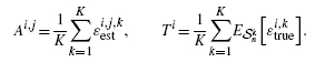
The problem of multiple-rule bias is exacerbated if one combines it with applying the multiple rules across multiple datasets (Yousefi et al., 2010) and then minimizes over both the classifier models and datasets; however, using multiple datasets can mitigate multiple-rule bias if performances are averaged over the datasets. In this case, each dataset is a sample from a feature-label distribution F_k, k = 1, 2, … , K, and our concern is with average performance over the K feature-label distributions. Assuming multiple error estimators, there are m classification rules being considered over the K feature-label distributions. Our interest is now with

(9)

where ϵ^{i, j, k}_est is the estimated error of classifier ψ_i and the error estimation rule Ξ_j on the dataset from feature-label distribution F_k. The bias takes the form

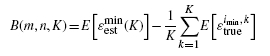(10)

where ϵ _true^{i_min, k} is the true error of classifier ψ _imin on the dataset from feature-label distribution F_k.

The ‘average’ curves in Figures 5 and 6 illustrate the effects of averaging. They show less estimation bias, less variance, smaller RMS and less comparative-performance bias when averaging is employed, as opposed to using the datasets individually. The situation is similar, albeit a bit more complicated, than the argument in Yousefi et al. (2010) for averaging results over a large number of datasets. Here, the averaging is done to mitigate multiple-rule bias.

It is possible to obtain theoretical results regarding the effect of averaging on the bias of Equation (10). In particular, if all error estimators are unbiased, then we prove in the Appendix A that lim_{K→ ∞}B(m, n, K) = 0. If one looks closely at the proof, it is clear that the unbiasedness assumption can be relaxed in each of the lemmas. In the first lemma, which shows that B(m, n, K) ≤ 0, we need only assume that none of the error estimators is pessimistically biased. In the second lemma, which shows that lim_{K→ ∞}B(m, n, K) ≥ 0, unbiasedness can be relaxed to weaker conditions regarding the expectations of the terms making up the minimum in Equation (9); however, these conditions are rather arcane and do not add much practical insight. Moreover, we are interested in close-to-unbiased error estimators, specifically, the cross-validation estimators, so that we can expect |B(m, n, K)| to diminish with averaging, even if the limit of B(m, n, K) does not actually converge to 0.

3.4 Concluding remarks

From a practical standpoint, the results obtained in the present paper quantitatively demonstrate the large degree of overoptimism that results from comparing classifier rule models via their performances on a small dataset owing to the inaccuracy of error estimation on small samples. As the array of simulations show, optimistic bias accrues rapidly with even a small number of models being compared. We have observed from both simulations and theoretical analysis that the problem can be mitigated by averaging performances across a family of datasets; indeed, this is the recommendation that we put forth. The downside is that averaging eliminates the possibility of comparing classification rule performances on a single population. In fact, the latter possibility has been precluded at the outset by the experimental design: too small of a sample to obtain accurate error estimates. If there is only a single small sample, then the multiple-rule bias precludes any conclusions whatsoever, whereas at least if a collection of datasets are employed, then one may be able to make a conclusion relative to the collection of populations (depending on the accuracy of the error estimator). Even with averaging, we must offer a word of caution. While the proposition we have proven regarding the convergence of B(m, n, K) is promising, like most distribution-free results it leaves open the rate of convergence, which in practice determines the number of datasets one must utilize to reduce the bias to some predetermined level. This leads us to some final comments.

The concerns expressed regarding the difficulty of establishing performance advantages for proposed classification rules (Boulesteix, 2010; Jelizarow et al., 2010; Rocke et al., 2009) reflect fundamental epistemological issues confronting bioinformatics as it addresses the high-throughput environment with limited sample sizes and limited statistical knowledge of how to deal with this new world (Dougherty and Braga-Neto, 2006; Dougherty, 2008; Mehta et al., 2004). The problem addressed in this article arises from the bias and variance, and therefore the RMS, of error estimators. Very little is known about the performance of common error estimators, in particular, cross-validation. To take a salient example: LOO. Prior to 2009, all that was known about LOO for LDA and Gaussian class-conditional distributions were asymptotic expressions for the expectation and variance of the estimator in one dimension (Davison and Hall, 1992). In 2009, the distribution of the LOO estimator was discovered in this model for an arbitrary dimension m without assuming a common variance for m = 1 and assuming a common covariance matrix with m>1 (Zollanvari et al., 2009). Still, none of these results treated the joint distribution of the estimated and true errors, nor, in particular, the RMS. In 2010, the joint distribution was found exactly for m = 1 without assuming a common variance and an approximation was found for m>1 assuming a common covariance matrix (Zollanvari et al., 2010). Besides the joint distribution via complete enumeration (Xu et al., 2006) and the correlation (Braga-Neto and Dougherty, 2010) for multinomial discrimination, there are no other analytic results regarding the joint behavior of LOO with the true error. This dearth of results is striking considering that LOO was first proposed in 1968 (Lachenbruch and Mickey, 1968), it has been used extensively, and the variance problems of LOO have been known from at least 1978 (Glick, 1978). As for more complicated cross-validation estimators that require random resampling, essentially nothing is known. If lamentations regarding the lack of performance characterization in bioinformatics are to be abated, then much greater knowledge regarding error estimation must be discovered.

Appendix A

We prove that if all error estimators are unbiased, then lim_{K→ ∞} B(m, n, K) = 0.

Lemma A.1. —

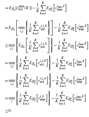
If all error estimators are unbiased, then B(m, n, K) ≤ 0.

Proof —

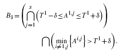
Define the set _n = {_n¹, _n², … , _n^K}, where _n^k, k = 1, 2, … , K is a random sample taken from the distribution F_k for k = 1, 2, … , K. Also, we can rewrite Equation (9) as

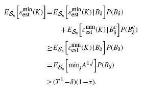
(A.1)

where i = 1, 2, … , r and j = 1, 2, … , s. Owing to the unbiasedness of the error estimators, E_n^k[ϵ^{i, j, k}_est] = E_n^k[ϵ^{i, k}_est]. Referring to Equations (10) and (A.1), we have

(A.2)

where the relations in the third and sixth lines result from Jensen's inequality and unbiasedness of the error estimators, respectively.□

Lemma A.2. —

If all error estimators are unbiased, then lim_{K→ ∞} B(m, n, K) ≥ 0.

Proof —

Let

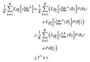
(A.3)

Owing to the unbiasedness of the error estimators, E_n[A^{i, j}] = Tⁱ ≤ 1. Without loss of generality, we assume T¹ ≤ T² ≤ … ≤ T^r. To avoid cumbersome notation, we will further assume that T¹≤T² (with some adaptation, the proof goes through without this assumption). Let 2δ = T² − T¹ and

(A.4)

Because | ϵ^{i, j, k}_est | ≤ 1, Var_n[A^{i, j}] ≤ 1/K. hence, for τ>0, there exists K_{δ, τ} such that K ≥ K_{δ, τ} implies P(B_δ(K)) > 1 − τ. Hence, referring to Equation (10), for K ≥ K_{δ, τ},

(A.5)

Again referring to Equation (10) and recognizing that i_min = 1 in B_δ, for K ≥ K_{δ, τ},

(A.6)

Putting Equations (A.5) and (A.6) together and referring to Equation (10) yields, for K ≥ K_{δ, τ},

(A.7)

Since δ and τ are arbitrary positive numbers, this implies that for any η>0, there exists K_η such that K ≥ K_η implies lim_K→∞ B(m, n, K) ≥ 0, which is precisely what we want to prove.□

Combining Lemmas A.1 and A.2, we have proven that lim_{K→ ∞} B(m, n, K) = 0 under the assumption that all the error estimators are unbiased.

REFERENCES

- Boulesteix A-L. Over-optimism in bioinformatics research. Bioinformatics. 2010;26:437–439. doi: 10.1093/bioinformatics/btp648. [DOI] [PubMed] [Google Scholar]
- Boulesteix A-L, Strobl C. Optimal classifier selection and negative bias in error rate estimation: an empirical study on high-dimensional prediction. BMC Med. Res. Meth. 2009;9:85. doi: 10.1186/1471-2288-9-85. [DOI] [PMC free article] [PubMed] [Google Scholar]
- Braga-Neto UM, Dougherty ER. Is cross-validation valid for small-sample microarray classification? Bioinformatics. 2004;20:374–380. doi: 10.1093/bioinformatics/btg419. [DOI] [PubMed] [Google Scholar]
- Braga-Neto UM, Dougherty ER. Exact performance of error estimators for discrete classifiers. Pattern Recognit. 2006;38:1799–1814. [Google Scholar]
- Braga-Neto UM, Dougherty ER. Exact correlation between actual and estimated errors in discrete classification. Pattern Recognit. Lett. 2010;31:407–412. [Google Scholar]
- Chen X, et al. Novel endothelial cell markers in hepatocellular carcinoma. Modern Pathol. 2004;17:1198–1210. doi: 10.1038/modpathol.3800167. [DOI] [PubMed] [Google Scholar]
- Davison AC, Hall P. On the bias and variability of bootstrap and cross-validation estimates of error rate in discrimination problems. Biometrika. 1992;79:279–284. [Google Scholar]
- Dougherty ER, Braga-Neto UM. Epistemology of computational biology: mathematical models and experimental prediction as the basis of their validity. J. Biol. Syst. 2006;14:65–90. [Google Scholar]
- Dougherty ER, et al. Validation of computational methods in genomics. Curr. Genomics. 2007;8:1–19. doi: 10.2174/138920207780076956. [DOI] [PMC free article] [PubMed] [Google Scholar]
- Dougherty ER. On the epistemological crisis in genomics. Curr. Genomics. 2008;9:69–79. doi: 10.2174/138920208784139546. [DOI] [PMC free article] [PubMed] [Google Scholar]
- Glick N. Additive estimators for probabilities of correct classification. Pattern Recognit. 1978;10:211–222. [Google Scholar]
- Hanczar B, et al. Decorrelation of the true and estimated classifier errors in high-dimensional settings. EURASIP J. Bioinform. Syst. Biol. 2007;2007:38473. doi: 10.1155/2007/38473. [DOI] [PMC free article] [PubMed] [Google Scholar]
- Hanczar B, Dougherty ER. On the comparison of classifiers for microarray data. Curr. Bioinformatics. 2010;5:29–39. [Google Scholar]
- Hanczar B, et al. Small-sample precision of ROC-related estimates. Bioinformatics. 2010;26:822–830. doi: 10.1093/bioinformatics/btq037. [DOI] [PubMed] [Google Scholar]
- Hua J, et al. Performance of feature selection methods in the classification of high-dimensional data. Pattern Recognit. 2009;42:409–424. [Google Scholar]
- Jelizarow M, et al. Over-optimism in bioinformatics: an illustration. Bioinformatics. 2010;26:1990–1998. doi: 10.1093/bioinformatics/btq323. [DOI] [PubMed] [Google Scholar]
- Lachenbruch PA, Mickey MR. Estimation of error rates in discriminant analysis. Technometrics. 1968;10:1–11. [Google Scholar]
- Mehta T, et al. Towards sound epistemological foundations of statistical methods for high-dimensional biology. Nat. Genet. 2004;36:943–947. doi: 10.1038/ng1422. [DOI] [PubMed] [Google Scholar]
- Natsoulis G, et al. Classification of a large microarray data set: algorithm comparison and analysis of drug signatures. Genome Res. 2005;15:724–736. doi: 10.1101/gr.2807605. [DOI] [PMC free article] [PubMed] [Google Scholar]
- Rocke DM, et al. Papers on normalization, variable selection, classification or clustering of microarray data. Bioinformatics. 2009;25:701–702. [Google Scholar]
- Shmulevich I, Dougherty ER. Genomic Signal Processing. Princeton: Princeton University Press; 2007. [Google Scholar]
- Xu Q, et al. Confidence intervals for the true classification error conditioned on the estimated error. Technol. Cancer Res. Treat. 2006;5:579–589. doi: 10.1177/153303460600500605. [DOI] [PubMed] [Google Scholar]
- Yeoh EJ, et al. Classification, subtype discovery, and prediction of outcome in pediatric acute lymphoblastic leukemia by gene expression profiling. Cancer Cell. 2002;1:133–143. doi: 10.1016/s1535-6108(02)00032-6. [DOI] [PubMed] [Google Scholar]
- Yousefi MR, et al. Reporting bias when using real data sets to analyze classification performance. Bioinformatics. 2010;26:68–76. doi: 10.1093/bioinformatics/btp605. [DOI] [PubMed] [Google Scholar]
- Zhan F, et al. The molecular classification of multiple myeloma. Blood. 2006;108:2020–2028. doi: 10.1182/blood-2005-11-013458. [DOI] [PMC free article] [PubMed] [Google Scholar]
- Zollanvari A, et al. On the sampling distribution of resubstitution and leave-one-out error estimators for linear classifiers. Pattern Recognit. 2009;42:2705–2723. [Google Scholar]
- Zollanvari A, et al. Joint sampling distribution between actual and estimated classification errors for linear discriminant analysis. IEEE Trans. Inform. Theory. 2010;56:784–804. [Google Scholar]
Associated Data
This section collects any data citations, data availability statements, or supplementary materials included in this article.