Identification of Human Gene Core Promoters in Silico

Abstract

Identification of the 5′-end of human genes requires identification of functional promoter elements. In silico identification of those elements is difficult because of the hierarchical and modular nature of promoter architecture. To address this problem, I propose a new stepwise strategy based on initial localization of a functional promoter into a 1- to 2-kb (extended promoter) region from within a large genomic DNA sequence of 100 kb or larger and further localization of a transcriptional start site (TSS) into a 50- to 100-bp (corepromoter) region. Using positional dependent 5-tuple measures, a quadratic discriminant analysis (QDA) method has been implemented in a new program—CorePromoter. Our experiments indicate that when given a 1- to 2-kb extended promoter, CorePromoter will correctly localize the TSS to a 100-bp interval ∼60% of the time.

[Figure 3 can be found in its entirety as an online supplement at http://www.genome.org.]

As the Human Genome Project enters its large-scale sequencing phase, methods for the identification of genes and regulatory elements in silico have become extremely important (Business Week 1996). In the past decade, many reliable in silico methods have been developed and used successfully (for review, see Claverie 1997) to identify protein coding regions; unfortunately, however, reliable methods for identifying either the 5′ or 3′ ends of gene transcript units are still lacking (for review, see Fickett and Hatzigeorgiou 1997). The inability to identify the 5′ and 3′ ends of genes using computational methods severely limits our ability to separate one gene from another when analyzing multigene fragments. Although the 3′ ends of many transcripts may be identified by searching the expressed sequence tags (ESTs), where 3′ end cDNA sequences are enriched, no rapid and accurate 5′ end gene sequencing method is yet available. Clearly a systematic improvement of computational promoter recognition methods is very much in need.

Recent advances in molecular genetics, biochemistry, and structural biology have revealed that RNAPII promoters typically have a modular structure, consisting of multiple short sequence elements, most of which comprise transcription factor (TF) binding sites. These elements, which can be either positive or negative, can be dispersed or can overlap and usually lie within the 1-kb region upstream and surrounding a transcription start site (TSS). The combination of these regulatory elements is often unique for most genes or pathways. Within this region lies a core promoter, typically from −60 to +40 bp relative to a TSS, defined by a minimal DNA element that is necessary and sufficient for accurate transcription initiation in a reconstituted cell-free system (Roeder 1996). The core promoter is responsible for binding the basal transcription factors and thus constitutes a universal positioning element within promoter regions. Transcription initiation is hierarchical and dynamic: It starts from chromosomal derepression (through chromatin remodeling and nucleosome discruption) and TF binding and results in the activation of transcription via a multitude interaction among the regulatory and basal TFs. Although a core promoter may be sufficient to direct transcription in vitro, a full intact promoter containing upstream sequence elements is often required for transcription in vivo.

Based on consideration of the biological knowledge of promoter architecture, a two-step approach to the computational problem of promoter recognition and TSS mapping was proposed recently (Zhang 1997b). Because hierarchical organization may dictate different molecular recognition mechanisms on different scale levels, this strategy essentially reduces the general promoter recognition problem into two related discrimination subproblems. The first subproblem is a large-scale (low-resolution) problem that may only need coarse-grained measures, such as CpG islands, nucleosome/chromatin features, downstream coding propensity, TF density, repetitive DNA counts, and so forth. The solution to this subproblem alone is enough for gene separation in principle, but it may have to await the availability of sufficient amount of long stretch genomic DNA sequence data. The second subproblem is a fine-scale (high-resolution) mapping problem that requires extracting detailed universal features that can best discriminate a core promoter from its surroundings. The solution to this subproblem also has immediate practical applications, especially for a bench scientist who has isolated and cloned a promoter activity into a 1- to 2-kb fragment. Currently, the human promoter–proximal data have just become sufficient enough for a systematic investigation. In a preliminary test (Zhang 1998), I had obtained very encouraging results on a small data set of 177 nonredundant human promoters in EPD48 (Bucher and Trifonov 1986). Here, I will show more robust results on a much larger data set of 673 nonredundant human promoters (see Data and Methods) and announce the availability of my new program CorePromoter to the genome community.

Core Promoter Architecture

Before going into computational aspects, it is helpful to briefly summarize core promoter structure (for more detailed reviews, see, e.g., Kollmar and Farnham 1993; Orphanides et al. 1996; Roeder 1996; Tjian 1996).

It is known that the TATA box and the Initiator (Inr) are the two key genetic elements in a core promoter (Fig. 1) that play a central role in determining the TSS position (e.g., Novina and Roy 1996). The TATA box has the consensus TATA(A/T)A(A/T), and the Inr has the consensus YYAN(T/A)YY (the underlined position indicates the TSS). TATA and Inr are functionally similar in two respects: Both can direct accurate transcription initiation by RNAPII in the absence of other control elements, and both can direct a high level of accurately initiated transcription when stimulated by an upstream activator (Smale 1997). Abundantly expressed genes (most cloned before 1980) frequently contain a strong TATA box in their core promoter. Housekeeping genes, oncogenes, growth factors, and TFs are often TATA-less. TATA⁻Inr⁺ promoters are mainly found in hematoietic lineage-specific genes and homeotic genes (Novina and Roy 1996), TATA⁻Inr⁻ promoters are mainly found in housekeeping genes that have multiple TSSs (often 40–80 bp downstream of a Sp1 site), and some share a downstream promoter element (DPE) called MED-1 with the consensus GCTCC(G/C) (Ince and Scotto 1995). Because of its overlap with other TF sites, Inr has much weaker consensus compared to the TATA box. Table 1 shows some experimentally mapped examples. Transcription initiation involves assembly of a preinitiation complex (PIC, see Fig. 1) on the core promoter. Although the details on the structure and organization are still lacking, recent site-specific protein–DNA photo-cross-linking done on a minimal human TBP–IIB–IIF–RNAPII–core promoter subcomplex has revealed that the interface between the largest and second largest subunits of RNAPII (RPBI and RPB2) forms an extended (∼240 Å) channel that interacts with core promoter DNA both upstream and downstream of TSS. (see also Forget et al. 1997; Lagrange et al. 1996). Although this mini-PIC covered at least the (−50, +20) region of the AdML core promoter, with TFIID a real PIC can bind a more extended region as measured by DNase I footprint (Orphanides et al. 1996). From this architectural information, it appeared that a core promoter might be localized in about the 100-bp region containing the TSS.

Figure 1.

Core promoter organization: (UPE and DPE) Upstream and downstream promoter elements; (X) a UPE-binding TF; (CIF) a Co–Inr TF; (A,B,D,F,E,H) TFIIA, TFIIB, etc.; (TBP) the TATA box-binding protein; (TF150 and TF250) TBP-associated factors (TAFs) 150 and 250, respectively.

Table 1.

Examples of TATA and TATA-Less Promoters

Gene	TATA box	Inr	TF
AdML	TATAAAA	TCACTCT	Pol II-I at (+7, +33)
gfa	CATAAAG	weak	Pol II-D at (+10, +50)
hsp70	TATAAAT	weak	Pol II-D at (+18, +30)
TdT	CTGCTGGTC	TCATTCT	Pol II-I, YY1
dhfr	—	CAAACTT	E2F
PBGD	—	TCAGTGT	? at (+3, +12)
rpS1	—	TCCCTTT	YY1
P5	—	CCATTTT	YY1

From Orphanides et al. (1996).  

RESULTS

Although it is known that the density of TF sites tends to be higher in promoter DNA than other genomic regions (this was actually the basis for many current promoter prediction algorithms; see, e.g., Prestridge 1995), a statisical study (Zhang 1998a) has shown that it is insufficient as an indicator of a core promoter. Most TF binding sites are not well localized, for the binding sites that were localized only in a statistical sense and mapped within a much broader region. Currently, the use of putative TF sites (those predicted by either consensus or matrix methods) will suffer at least from the following limitations: They lose important context information, many false positives, score/cutoff dependency, or the TF database is simply too limited or biased (as most of TF sites are not mapped and it will take years to map the majority of them experimentally). It is therefore more logical to start an objective statistical approach without having to resort to any putative TF site information directly and let the data speak for itself. Thus, a baseline is provided for further improvement by adding explicit TF site information later. As illustrated below, this approach has proved successful.

Exploratory LDA Studies with a Set of Nonoverlapping Windows

First, a k-tuple frequency measure was chosen. A global 6-tuple frequency measure had been used for promoter prediction as a “content” measure in the sense of Staden (Hutchinson 1996). But this content approach disregards all the positional information that is crucial for the fine mapping of the core promoter and TSS. In contrast, a pure “signal” approach is powerless because of the large variation in the signal positions. This suggests that a “mixed” approach, using position-specific windows, should present a suitable solution to the problem. Discriminant analysis is a standard statistical pattern recognition techique that has been used widely in many fields (see, e.g., McLachlan 1992). Intuitively, if one views samples as swarms of points in multidimensional feature space, discriminant analysis will provide an optimal surface (in the sense of minimizing errors) separating the true samples from the pseudosamples. When the surface is a plane, the method is called linear discriminant analysis (LDA); if it is quadratically curved, it is called quadratic discriminant analysis (QDA). LDA is often used for exploratory studies for its simplicity. When LDA is used, it is implicitly assumed that the true samples and the pseudosamples have the same covariance structure (see, e.g., Zhang 1997a). Here I chose the average k-tuple frequency preference score x in a window of size w as the feature variable (see Data and Methods).

Then there was the choice of k and w. Reliable statistics requires N × (w − k + 1) be larger than 4k, where N is the number of independent sequences, as w determines the resolution and it needs to be large enough to contain major TF elements but small enough to capture the positional variation. It was found experimentally that w = 30 bp works well even for the small Eukaryotic Promoter Database data set (N = 177). Although k = 6 may be barely workable, I chose a more cautious value of k = 5, which also represents a half-turn of a DNA double helix and often corresponds to the number of residues in the core of a typical TF binding site. For an exploratory test, I chose four nonoverlapping windows (hence, four feature variables) and did various LDA studies by varying different parameters (w, k, sample size, sampling interval, or adding other feature variables). These window positions were carefully chosen such that the first window would contain UPE, the second window would contain TATA box, the third window would contain Inr, and the last window would contain DPE (see Fig. 1). There was no need to separate TATA and TATA-less promoters, as the second feature variable would code this information differentially. The top half of Figure 2 shows some typical LDA discriminant score profiles (which have the meaning of the posterior probability that the window surrounding each position contains a core promoter) for 10 extended promoters from EPD48. The samples of prediction were taken at 6-bp intervals when scanning a sequence. A vertical line indicates the true TSS position (a comparison with PROSCAN, a TF density-based prediction, can be found in Zhang 1998). Although there is still significant noise in these profiles, the true signals stand out not only because of their height, but also because of their unique shape.

Figure 2.

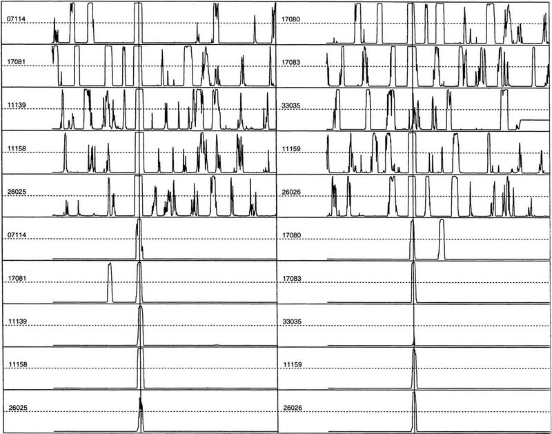
Top panels are LDA profiles for 10 extended EPD48 human promoter sequences. Bottom panels are QDA profiles for the same 10 sequences. The EPD entry-ID is indicated for each sequence. The vertical lines are the true TSS positions. The sequence range is (−600, +600). A peak in the profile indicates a high likelihood for a TSS.

A QDA Study with Two Overlapping Sets of Windows

How could the noise be reduced? More experiments indicated that the false positives were much more sensitive to change of parameters. When the window size or position is varied, true signals tend to remain at the same position while the noises tend to displace randomly (data not shown). This finding immediately suggested that it may be beneficial to apply the “principle of resonance”: If two profiles corresponding to different parameters are combined, the true signals will tend to enhance each other while the noises will tend to cancel each other. Furthermore, as the sample size is increased, the height of the noise tends to be suppressed. To maintain a high resolution as well as to limit the dimension of the multivariate feature space, I used the 13-window system (8 windows of 30 bp and 5 windows of 45 bp) with a sample size of 240 bp. Because the overlapping windows were used (see Fig. 6, below), a more covariance-sensitive method—QDA—was applied (see, e.g., Zhang 1997a). The bottom half of Figure 2 shows the new discriminant profiles obtained by QDA of 13 feature variables on the same 10 extended EPD48 promoters (see Data and Methods). The remarkable enhancement of the signal-to-noise ratio indicates that the “interference amplification” is at work.

Figure 6.

Feature variables in discriminant analyses.

To further analyze the stability (robustness), standard 10 cross-validation tests were performed on 177 true samples and 42,480 pseudosamples (20% test set and 80% training-set were chosen randomly in each test). The statistical variation is summarized in Table 2. In particular, the average sensitivity and specificity may be calculated as 0.71 and 0.83, respectively.

Table 2.

Cross-Validation Statistics

Testa	1	2	3	4	5	6	7	8	9	10
Sensitivity	0.857	0.771	0.629	0.571	0.657	0.771	0.657	0.686	0.629	0.857
Specificity	0.857	0.871	0.815	0.800	0.852	0.771	0.885	0.828	0.880	0.769

^a(Sensitivity) True Positives/actual positives; (specificity) true positives/predicted positives. 

Some interesting observations from these profiles are worth mentioning. The double peaks of the profiles in Figure 2 correspond to the alternative TSSs, as annotated in GenBank. Because, for simplicity, only one sample at position (−160, +80) per sequence was considered as the true sample (signal) and some alternative TSSs and the high scoring samples in the neighborhood of the true sample were considered as false positives (noise), it would be more informative to look at the whole profile. This QDA study involved only the position-dependent 5-tuple frequency bias. As the local background (as characterized by f_b in Data and Methods) was used, chromosomal GC content variation was therefore taken care of automatically. It was somewhat surprising that adding TATA or Inr scores as extra discriminant feature variables did not make any noticeable improvement (data not shown). Apparently they were also automatically built in by the specific choice of window positions. Actually, we believe that most, if not all, of the hidden positioning elements should be accommodated.

Enlargment of the Data Set and Implementation of Core Promoter

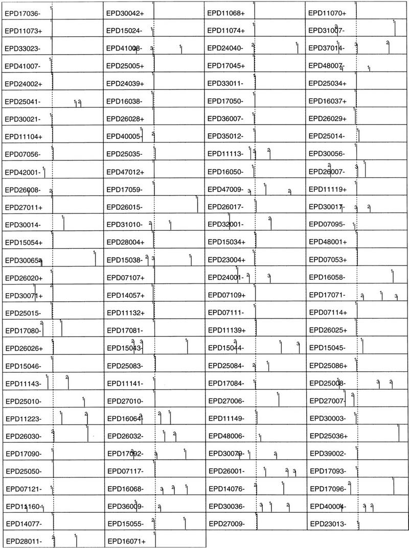
Because the human EPD data is very limited and is biased by TATA box-containing promoters (Zhang 1998a), a larger data set (673 promoters) was constructed based on a nonredundant first exon database (see Data and Methods). Because these promoters in the (−600, +600) region were taken from GenBank solely based on the TSS annotation, the data may be understandably more error-prone than EPD but they are more representative. Exactly the same procedure was carried out, and new sample means and covariance matrices were calculated from the true core promoters in the (−160, +80) region and from all of the pseudopromoters outside the (−240, +240) region where 240 bp was the size of a sample. The QDA posterior probability score profiles were plotted on a log10 scale (ranging from −3 to 0) in Figure 3 (40 sample profiles are shown; the complete 673 profile can be found at http://www.cshl.org/genefinder). To maximize the information content, I chose the following representation: Among the top 20 scores in the (−600, +600) region, only up to 3 top profile peaks are shown. That is, if the highest peak falls into the (−50, +50) region, only this one peak (marked by 1) is shown; if the second peak falls into the true neighborhood, only these two peaks (marked by 1 and 2) are shown, and so forth. The original GenBank accession number and the position of the TSS for each promoter are also indicated on the far left for ease of reference.

Figure 3.

QDA profiles (in log10 scale) for a newly constructed nonredundant human promoter database LEDB (673 sequences with 55 identical to EPD sequences) were depicted by up to the three highest peaks (see text for details). The GenBank accession no. and the TSS position are indicated at left. Each peak is also indicated by its rank number: (1) the highest peak in the whole profile, (2) the second highest, etc. The sequence range is (−600, +600), and the true TSS position is indicated by a vertical dotted line.

As expected, the accuracy for this larger data was reduced when compared with that for EPD data. In the correct neighborhood (−50, +50), 66% of the core promoters demonstrate the highest peaks; 81% if including also the second highest; 84% if further including the third highest. In addition, although the majority of the highest peaks are mapped closely to the core promoter region, the variation of the absolute value from one promoter to another can be very large (up to two orders of magnitude, which is why a logarithmic scale was used to plot the profile peaks).

To get the worst-case scenario, the QDA predictor constructed from the large data was used to make core promoter predictions on 122 extended EPD promoter sequences (a true test set) that did not intersect with the larger data. The result is shown in Figure 4. The range of these extended EPD promoters is also (−600, +600). Now, in the correct neighborhood (−50, +50), only 59% of the core promoters demonstrate as the highest peaks; 67% if including also the second highest; 73% if further including also the third highest. This may be regarded as a measure of the base-line statistic: in a novel extended promoter sequence (∼1.2 kb), a core promoter is expected to be localized correctly in a 100-bp region with at least 60% chance by this pure statistical QDA predictor without using any TF site information. Although many of the high peaks outside the 100-bp region turned out to be alternatively annotated core promoters, there was not enough information and resource to examine all of the false positives at that point.

Figure 4.

Similar QDA profiles to those in Fig. 3 for the 122 extended EPD promoters that were not used as the training set. (1) A strong TATA promoter.

To compare with the most similar available approach, I used TSSG (Solovyev and Salamov 1997) through the e-mail server at service@bchs.uh.edu. TSSG uses a LDA approach, and the feature variables are (1) a TATA box score, (2) triple preferences around the TSS, (3) hexamer preferences in the nonoverlapping regions (−300, −201), (−200, −101), and (−100, −1), and (4) potential transcription factor binding sites. For the 673 promoters, TSSG was only able to localize 37% in the (−50, +50) interval and 44% in the (−100, +100) interval. The novel features that may contribute to a better performance of CorePromoter are the overlapping set of relatively shorter windows and QDA.

As it is relatively easy to predict strong TATA promoters, to determine whether the correct prediction was correlated with such strong TATA promoters, a plus sign (+) was added next to the EPD entry-ID in each profile to indicate that sequence is a strong TATA promoter. A strong TATA promoter was defined by a score larger than the cutoff value of −2.2 when using the TATA box scoring matrix of Bucher (1990) near the −30 region (see Zhang 1998a for more on core promoter classification). As expected, most strong TATA promoters did have a high core promoter peak. This correlation may be seen more clearly in Figure 5 where the peak scores (on a log10 scale) in the (−50, +50) region of Figure 4 were plotted against the TATA scores. When the TATA score is larger than about −5 (−5.43 was the mean TATA score of the total 177 human EPD promoters; see Zhang 1998a), there appears to be a weak linear correlation that may have also caused the order of magnitude variation in peak scores. But the QDA predictor was able to predict many TATA-less core promoters, albeit with a reduced overall score level that was still clearly above the noises.

Figure 5.

The scatter plot of QDA scores (in log10 scale) for the peaks in (−50, +50) in Fig. 4 vs. the TATA scores (see text for detail).

Initially, this QDA algorithm is implemented in CorePromoter with the covariance matrix calculated from the 673 promoters (the EPD covariance matrix is an option). It may be accessed through the World Wide Web at http://www.cshl.org/genefinder, or it may be down-loaded from ftp://cshl.org/pub/science/promoter (the FTP version has the option for output of all the scores so that one can plot the whole profile locally). A more detailed study between the differences will be published elsewhere, and the future version of CorePromoter will contain the combined covariance matrix. I appeal to bench scientists for more accurate database annotations and for helping to correct errors. I have presented the TSS prediction in detail in both Figures 3 and 4 and sincerely hope to get feedback from biologists who are studying these genes. A statistical method can only achieve the same level of accuracy as that of a human annotator—perhaps with much greater efficiency. Without the help of the bench scientists, we have no way of knowing which are real true/false positives. CorePromoter will be improved further by adding more explicit TF site information in the future. As many gene-specific features were averaged out for the general purpose of core promoter recognition and fine TSS mapping, using gene-specific methods will be essential for any regulatory function studies.

DATA AND METHODS

One hundred seventy-seven human nonredundant promoter sequences were extracted from EPD48 (Bucher and Trifonov 1986). Each sequence was then extended from the original range (−500, +100) to (−600, +600) by the use of BLAST (GenBank, release 100). A few corrections were made after checking against both the original and recent publications. A larger promoter data set (673 sequences, called LEDB for lead exon database in CorePromoter options) was extracted (or extended when necessary) from a nonredundant first exon (including the flanking regions) database, which was constructed according to GenBank annotations (Zhang 1998b). The range for this data was also (−600, +600).

Standard LDA and QDA (see e.g., Zhang 1997a and references therein) were used for core promoter discrimination. All feature variables were 5-tuple scores averaged within a position-specific window. If one defines f_w(s) to be the signal frequency of a 5-tuple s in the window w and f_b(s) to be the background frequency calculated as the average of f_L(s) and f_R(s), where L and R indicate the left and the right nearest-neighbor nonoverlapping windows, then the 5-tuple score x(s) = f_w(s)/[f_w(s) + f_b(s)]. All the f_ws were estimated from the aligned data, and Bayesian priors were used to render all frequencies nonzero (Tanner and Wong 1987).

In the exploratory LDA studies, each sample was a sequence of 120 bp that contained four nonoverlapping windows of 30 bp each (Fig. 6). Samples for the training set were drawn from the 177 EPD48 nonredundant human sequences at a 10-bp interval. Each sequence would contain just one true sample (ignoring the few alternative TSSs) at (−70, +50).

REFERENCES

- Bucher P. Weight matrix descriptions of four eukaryotic RNA polymerase II promoter elements derived from 502 unrelated promoter sequences. J Mol Biol. 1990;212:563–578. doi: 10.1016/0022-2836(90)90223-9. [DOI] [PubMed] [Google Scholar]
- Bucher P, Trifonov EN. Compilation and analysis of eukaryotic POL II promoter sequences. Nucleic Acids Res. 1986;14:10009–10026. doi: 10.1093/nar/14.24.10009. [DOI] [PMC free article] [PubMed] [Google Scholar]
- Business Week. Sept. 2, 1996. Hunting through the “garbage” for DNA.Business Week. Sept. 2, 1996. Hunting through the “garbage” for DNA.
- Claverie J-M. Computational methods for the identification of genes in vertebrate genomic sequences. Hum Mol Genet. 1997;6:1735–1744. doi: 10.1093/hmg/6.10.1735. [DOI] [PubMed] [Google Scholar]
- Fickett JW, Hatzigeorgiou AG. Eukaryotic promoter recognition. Genome Res. 1997;7:861–878. doi: 10.1101/gr.7.9.861. [DOI] [PubMed] [Google Scholar]
- Forget D, Robert F, Grondin G, Burton ZF, Greenblatt J, Coulombe B. RAP74 induces promoter contacts by RNA polymerase II upstream and downstream of a DNA bend centered on the TATA box. Proc Natl Acad Sci. 1997;94:7150–7155. doi: 10.1073/pnas.94.14.7150. [DOI] [PMC free article] [PubMed] [Google Scholar]
- Hutchinson GB. The prediction of vertebrate promoter regions using differential hexamer frequency analysis. Corp Appl Bio Sci. 1996;12:391–398. doi: 10.1093/bioinformatics/12.5.391. [DOI] [PubMed] [Google Scholar]
- Ince TA, Scotto KW. A conserved downstream element defines a new class of RNA polymerase II promoters. J Biol Chem. 1995;270:30249–30252. doi: 10.1074/jbc.270.51.30249. [DOI] [PubMed] [Google Scholar]
- Kollmar R, Farnham PJ. Site-specific initiation of transcription by RNA polymerase II. Proc Exp Biol Med. 1993;203:127–139. doi: 10.3181/00379727-203-43583. [DOI] [PubMed] [Google Scholar]
- Lagrange T, Kim TK, Orphanides G, Ebright YW, Ebright RH, Reinberg D. High-resolution mapping of nucleoprotein complexes by site-specific TBP-TFIIA-TFIIB-DNA quaternary complex. Proc Natl Acad Sci. 1996;93:10620–10625. doi: 10.1073/pnas.93.20.10620. [DOI] [PMC free article] [PubMed] [Google Scholar]
- McLachlan GJ. Discriminant analysis and statsitical pattern recognition. New York, NY: Wiley; 1992. [Google Scholar]
- Novina CD, Roy AL. Core promoters and transcription factor binding sites. J Mol Biol. 1996;249:923–932. doi: 10.1006/jmbi.1995.0349. [DOI] [PubMed] [Google Scholar]
- Orphanides G, Thierry L, Reinberg D. The general transcription factors of RNA polymerase II. Genes & Dev. 1996;10:2657–2683. doi: 10.1101/gad.10.21.2657. [DOI] [PubMed] [Google Scholar]
- Prestridge DS. Prediction Pol II promoter sequences using transcription factor binding sites. J Mol Biol. 1995;249:923–932. doi: 10.1006/jmbi.1995.0349. [DOI] [PubMed] [Google Scholar]
- Roeder RG. The role of general initiation factors in transcription by RNA polymerase II. Trends Biochem Sci. 1996;21:327–335. [PubMed] [Google Scholar]
- Smale ST. Transcription initiation from TATA-less promoters within eukaryotic protein-coding genes. Biochim Biophys Acta. 1997;1351:73–88. doi: 10.1016/s0167-4781(96)00206-0. [DOI] [PubMed] [Google Scholar]
- Solovyev V, Salamov A. The Gene-Finder computer tools for analysis of human and model organism genome sequences. In: Gaasterland T, Karp P, Karplus K, Ouzounis C, Sander C, Valencia A, editors. Proceedings of the 5th International Conference on Intelligent Systems for Molecular Biology. Menlo Park, CA: AAAI Press; 1997. pp. 294–302. [PubMed] [Google Scholar]
- Tanner MA, Wong WH. The calculation of posterior distribution by data augmentation. J Am Stat Asoc. 1987;82:528–550. [Google Scholar]
- Tjian R. The biochemistry of transcription in eukaryotes: A paradigm for multisubunit regulatory complexes. Philos Trans R Soc Lond B Biol Sci. 1996;351:491–499. doi: 10.1098/rstb.1996.0047. [DOI] [PubMed] [Google Scholar]
- Zhang MQ. Identification of protein coding regions in the human genome by quadratic discriminant analysis. Proc Natl Acad Sci. 1997a;94:565–568. doi: 10.1073/pnas.94.2.565. [DOI] [PMC free article] [PubMed] [Google Scholar]
- ————— . Georgia Tech International Conference on Bioinformatics: Gene discovery in silico. Nov. 6–9. Atlanta, GA: Georgia Tech University; 1997b. On a new strategy of promoter recognition. [Google Scholar]
- ————— . A discrimination study of human core-promoters. In: Altman R, Donker AK, Hunter L, Klein TE, editors. Proceedings of Pacific Symposium on Biocomputing ’98. Jan. 4–9. Maui, Hawaii. Singapore: World Scientific; 1998a. pp. 240–251. [Google Scholar]
- ———. 1998b. Statistical features of human exons and their flanking regions. Hum. Mol. Genet. (in press). [DOI] [PubMed]