Patterns of Chromosomal Duplication in Maize and Their Implications for Comparative Maps of the Grasses

Abstract

The maize genome contains extensive chromosomal duplications that probably were produced by an ancient tetraploid event. Comparative cereal maps have identified at least 10 duplicated, or homologous, chromosomal regions within maize. However, the methods used to document chromosomal homologies from comparative maps are not statistical, and their criteria are often unclear. This paper describes the development of a simulation method to test for the statistical significance of marker colinearity between chromosomes, and the application of the method to a molecular map of maize. The method documents colinearity among 24 pairs of maize chromosomes, suggesting homology in maize is more complex than represented by comparative cereal maps. The results also reveal that 60%–82% of the genome has been retained in colinear regions and that as much as a third of the genome could be present in multiple copies. Altogether, the complex pattern of colinearity among maize chromosomes suggests that current comparative cereal maps do not adequately represent the evolution and organization of the maize genome.

The maize genome contains extensive chromosomal duplication. The first hints of duplication came from cytological studies (McClintock 1930, 1933; Snope 1967; Ting 1966) that were later corroborated by linkage studies (Rhoades 1951, 1955; Goodman et al. 1980; McMillin and Scandalios 1980; Wendel et al. 1986, 1989). However, the extent of duplication was not appreciated fully until the advent of molecular maps (Helentjaris et al. 1988; Ahn and Tanksley 1993). Comparative mapping studies have identified roughly 10 duplicate (or homologous) chromosomal regions in maize, all of which share homology with a rice chromosome (Ahn and Tanksley 1993; Moore et al. 1995a; Gale and Devos 1998a; Wilson et al. 1999). The extent of chromosomal duplication suggests that maize, a diploid with 10 chromosomes (2x = 20), had a polyploid origin (Anderson 1945; Rhoades 1951; Helentjaris et al. 1988; Gaut et al. 2000).

Characterizing patterns of chromosomal duplication within maize contributes to our understanding of genome relationships among grasses (Bennetzen and Freeling 1993, 1997; Gale and Devos 1998b). Genome relationships among grasses ostensibly provide a basis for predicting the location of functionally important genes (Leister et al. 1998; Peng et al. 1999). However, the current methods used to identify chromosomal homology from molecular maps have serious shortcomings. The most important shortcoming is the lack of objective criteria for identifying duplicated regions. In some cases, investigators rely on the poorly defined (Passarge et al. 1999) concept of synteny (in this context, shared molecular markers between chromosomes) to define regions of chromosomal homology, and in other cases colinearity (shared markers and shared order) is used as evidence for chromosomal duplications. Even when the more rigorous concept of colinearity is used, individual studies are often unclear as to the number and distribution of colinear markers that are used to define homologous regions.

This study outlines the development of a simulation method to test for the statistical significance of marker colinearity between chromosomes and the application of the method to the UMC98 map (Davis et al. 1999), the largest molecular marker map of maize to date. Colinearity tests indicate that homology among maize chromosomes is more extensive than previously documented. The results have important implications for understanding the organization and evolution of the maize genome.

METHODS AND RESULTS

The Colinearity Test

The test is based on the premise that colinear runs of markers can reflect either randomness (statistical noise) or underlying genome organization. The basic idea of the test is to determine whether a run of n colinear markers is expected at random and, if so, whether the observed run of n markers is more clustered on the genetic map than expected at random. The test requires four steps: (1) Defining a colinear run, (2) measuring a colinear run, (3) identifying all colinear runs between two chromosomes, and (4) testing the significance of observed colinear runs.

Step 1—Defining Colinearity

Colinearity refers to markers that cross-hybridize to two chromosomes and retain linear order on both chromosomes. Figure 1 is based on the UMC98 map of chromosome 1 (Davis et al. 1999) and illustrates cross-hybridizing markers between chromosome 1 and the nine other maize chromosomes. All nine maize chromosomes share colinear markers with chromosome 1. In some cases, there are many colinear markers between chromosomes—for example, chromosomes 1 and 5 share ≈20 cross-hybridizing markers that are ordered on both chromosomes. In other cases, there are few colinear markers between chromosomes—for example, at most three markers cross-hybridize to chromosomes 1 and 10 and retain order on both chromosomes. The challenge of these data is to determine which sets of colinear markers are statistically significant.

Figure 1.

A diagram of the UMC98 map of chromosome 1 showing markers that cross-hybridize between chromosome 1 and the other nine chromosomes. The vertical axis is the map position on chromosome 1. Black lines indicate markers mapped to chromosome 1, the standard chromosome; markers that cross-hybridize to other chromosomes are shown in gray with their map position(s) on the tester chromosome. Parentheses indicate the number of markers mapped to the same location.

In Figure 1, chromosome 1 is defined as the standard chromosome because the figure is based on the map of chromosome 1; the other nine chromosomes are defined as tester chromosomes. Note that nine figures analogous to Figure 1 can be drawn, with each figure based on the UMC98 map of a different maize chromosome. Thus, each chromosome can be represented separately as the standard chromosome. It is important to represent each chromosome as a standard because colinearity depends on which chromosome is the standard and which is the tester (Fig. 2).

Figure 2.

Colinearity depends on which chromosome is the standard and which is the tester. Each row shows the centimorgan location of a hypothetical marker that cross-hybridizes to two chromosomes. (Gray arrows) Colinear runs of markers between the chromosomes. (A) With chromosome I as the standard, a colinear run contains six markers. (B) With chromosome II as the standard, the longest run has four markers. Such asymmetry is common in maize data and probably represents intrachromosomal rearrangements.

Map data such as those shown in Figure 1 have three characteristics that can complicate recognition of colinearity. The first characteristic is that the same marker can map to more than one position on a single chromosome, and hence one must choose which map position best retains colinearity (Fig. 3A). The second characteristic is that multiple markers can map to a single position, particularly when markers are assigned to “bins.” Markers within bins can be rearranged to maximize the number of markers in a colinear run (Fig. 3B). Finally, mapping error can cause the linear order of markers to be assigned incorrectly, but map error can be included in definitions of colinearity (Fig. 3C). In this study, the first two characteristics were always included in the definition of colinearity, but analyses were performed with and without recognition of map error (see below).

Figure 3.

Colinearity based on hypothesized map data from seven markers that cross-hybridize between chromosomes 1 and 5. (A) Marker II hybridizes to two positions on chromosome 1 (153.7 and 207.3 cM). Based on the position of marker II at 207.3 cM, markers I through III define a colinear run of three markers (gray arrow). Some additional colinear runs of n = 2 markers are also shown. (B) Markers V, VI, and VII are binned at 196.1 cM on chromosome 1, and hence their order is ambiguous. Markers VI and V (in boldface) can be rearranged to maximize the number of markers in a colinear run. (C) Maps contain statistical error in the assignment of linear order. If the potential error extends 2.0 cM in either direction of a marker, then the relative position of markers III and IV (in boldface) are uncertain on chromosome 5 because of their close location. A colinear run can extend through these markers in recognition of map error, resulting in a colinear run of seven markers. Recognition of error must be applied to both chromosomes. (D) A simulated data set showing randomized centimorgan locations on tester chromosome 5 (in boldface). The simulated data result in two colinear runs of n = 4 and n = 2 markers (gray arrows).

Step 2—Measuring Colinear Regions

Colinear runs have two features: The number of markers in the run and the centimorgan distance covered by the run. Both characteristics need to be considered to determine a run's significance. The number of markers in a colinear run is straightforward—for example, given a definition of colinearity that includes map error, Figure 3C contains a run of seven markers. The genetic distance covered by a run can be measured by many possible metrics. Four metrics were explored in this study:

1. The total distance of the run, d, is the absolute value of the run's length, in centimorgans, summed over both chromosomes. For example, Figure 3C contains a run of seven markers with d = (209.2 − 196.1) + (50.0 − 29.8) = 33.2 cM.

2. The sum of squares distance, ss, is squared centimorgan length of the run, summed over both chromosomes. Figure 3C has a run with ss = (209.2 − 196.1)² + (50.0 − 29.8)² = 579.65 cM².

3. The sum of the variances, var, is the sampling variance of the centimorgan location of markers in a run, summed over both chromosomes. In Figure 3C, the sampling variance of the seven markers on chromosome 1 is 30.62, and the sampling variance for markers on chromosome 5 is 85.65, and var = 30.62 + 85.65 = 116.30.

4. The pairwise difference measure, pr, is defined as

   

   where n is the number of markers in a run, and x and y are the centimorgan marker positions on two chromosomes under comparison. The pr metric for the colinear run in Figure 3C is 6.65 + 10.82 = 17.47.

Step 3—Identifying Colinear Runs

Colinear runs were identified between the standard chromosome and a tester chromosome with the following procedure. First, the colinear run(s) containing the highest number of genetic markers, n, was identified, and the appropriate metric (d, ss, var, or pr) was calculated. Second, markers in the colinear run(s) of n markers were removed from further consideration. This practice ensured that each genetic marker belonged to one and only one colinear run. If two runs each had n markers but shared markers in common, the run with the smallest metric was defined first. Third, the process was repeated for runs of n-1 markers, n-2 markers, and so on until n = 2 and all colinear runs were defined between chromosomes. For each data set, run definition was performed for the standard chromosome against all nine tester chromosomes.

Step 4—Testing Significance

A simulation procedure was used to test the null hypothesis that a colinear run is a random collection of markers. Simulation randomized the position of cross-hybridizing markers on tester chromosomes, while retaining the position of markers on the standard chromosome (Fig. 3D). The new locations were drawn from a uniform deviate between 0.0 and the centimorgan length of the tester chromosome. For example, the map length of maize chromosome 2 is 207.6 cM, and thus cross-hybridizing markers on chromosome 2 were randomly assigned a position between 0.0 and 207.6 cM for each simulation. Diagrammatically, each simulation corresponds to holding the positions of the gray markers in Figure 1 constant but assigning each marker a new centimorgan location.

For each standard chromosome, simulations were performed 10,000 times. For each simulated data set, colinear runs were identified and measured on all nine tester chromosomes relative to the standard chromosome. The probability of an observed run was scored as the proportion of simulated data sets that had a colinear run with the same number of markers and a smaller metric on the same two chromosomes. A run was considered significant with probability P ≤ 0.05.

Implementation

The colinearity tests were implemented in a C-program and applied to UMC98 data (Davis et al. 1999) compiled from MaizeDB (www.agron.missouri.edu) in September 1999. The test was applied with all four metrics and two different error allowances: no allowance, which essentially assumes there was no error in the linear order of UMC98 markers, and an error allowance of 2.0 cM in either direction from a marker, which roughly approximates the 95% confidence of centimorgan location in the UMC98 map (Davis et al. 1999). Ten data sets were tested, each corresponding to a different maize chromosome as standard. With a map error of 0.0 cM, markers within bins were rearranged exhaustively to identify colinear runs (Fig. 3B). With a map error of 2.0 cM, exhaustive rearrangement proved computationally prohibitive on rare occasions, due to a high number of markers located within 2.0 cM of one another. When exhaustive rearrangement was prohibitive, the best of 100,000 rearrangements was chosen.

One concern about the colinearity approach is that many colinear runs can be identified between one standard chromosome and the nine tester chromosomes (Figs. 1, 3). Because each colinear run is examined for significance, there is the potential that significance values require a multiple test correction. The type I error should be 0.05 for each data set (i.e., each standard chromosome against its nine tester chromosomes) and not for individual colinear runs. The simulation design should adequately correct type I error, but I verified correct type I error by simulation. Type I simulations were based on a total of 1000 randomized UMC98 data sets, with 100 data sets representing each of the 10 standard chromosomes. Because randomized data sets represent the null hypothesis of random marker order, only 5% should contain significant colinear runs. Altogether, 50 of 1000 data sets contained one or more significant colinear runs, and this is the number expected with a type I error of 0.05. Within groups of 100 data sets, the number of significant data sets ranged from three to seven; none of these deviations was significantly different from the expected number of five. Thus, simulations verify that the approach adequately corrects for testing multiple colinear runs within a single data set.

Comparing Metrics and Map Error Allowances

To investigate properties of the method, colinearity tests were performed on UMC98 data with all four metrics (d, ss, pr, and var) and two different map error allowances (0.0 and 2.0 cM). It is not obvious a priori which metric is most reasonable, because the metrics capture slightly different properties of colinear runs. Nonetheless, the metrics performed similarly. For example, when map error was 0.0 cM, a total of 243 colinear runs were identified over the 10 data sets representing the 10 standard chromosomes. Of these 243 runs, 60 were significant with the ss metric, and a subset of 57 of the 60 was significant with the d metric. Thus, the d and ss statistics agreed in the significance (or lack thereof) for 240 of 243 = 98.8% of the colinear runs. Similarly, var and pr agreed in 95.6% of runs. The lowest level of agreement was between the ss and pr metrics, but these still agreed for 93.0% of runs. Altogether, results were largely robust to the choice of metric, and runs that were not consistently significant between metrics were usually marginally significant (0.05 < P <  0.10) with other metrics. Because of this robustness, the remainder of this paper focuses only on the ss metric, which is a function of the relative centimorgan length of a run on both chromosomes and has the merit of simplicity.

The level of map error fundamentally changes the definition of colinearity (Fig. 2B,C), resulting in a different number of colinear runs to be tested depending on the defined level of error. With higher error, colinear runs tend to be longer, and hence there are fewer total runs; 215 runs were defined over all 10 data sets when mapping error was 2.0 cM, whereas 243 runs were detected when map error was 0.0 cM. However, the total proportion of significant runs was similar when map error was 0.0 and 2.0 cM. Over all 10 data sets, 60 of 243 (24.6%) of the observed runs were significant when map error was 0.0 cM, and 52 of 215 (24.2%) of the runs were significant when map error was 2.0 cM. One difference between error treatments was that as few as two markers could constitute a significant colinear run when map error was 0.0 cM, whereas runs with more markers (n ≥ 3) were needed for a colinear run to be significant with a 2.0-cM map error. As a consequence, the 0.0 cM error treatment detected colinearity between more pairs of chromosomes. With a 0.0 cM error, a total of 27 of 45 possible chromosomal pairs had colinear associations, whereas 24 chromosomal pairs had associations with an error rate of 2.0 cM. These results indicate that a map error of 2.0 cM is more conservative with the UMC98 data, and thus the remainder of the study focuses on results based on a map error of 2.0 cM.

Colinearity between Maize Chromosomes

The centimorgan map locations and P values of runs based on the ss metric and a 2.0-cM error allowance are given (Table 1). Fifty-two significant runs were detected at P ≤ 0.05 (Fig. 4); these colinearities were located on 24 pairs of chromosomes (Table 2). When the P value was Bonferroni-corrected to P ≤ 0.005 for a type I error of 0.05 over all 10 data sets, the number of significant colinear runs reduced to 25 runs (Fig. 4) located on 17 chromosomal pairs (Table 2). The issue of significance level deserves comment. The Bonferroni-corrected significance level (P ≤ 0.005) is more stringent, but results at the level of data set (P ≤ 0.05) corroborate observations from the literature (Table 2) and also provide information for further investigation. Given these considerations and the inherently conservative nature of the results (see Discussion), both levels of significance are reported here.

Table 1.

Colinear Runs and Associated P Values for Runs Detected with ss Metric and a Mapping Error of 2.0 cM

Stda	Std (cM)b	Testc	Test (cM)d	⧣Marke	P valuef	Symmetryg
1	205.2–241.3	5	5.1–39.4	13	0.0001	S
1	164.6–202.1	5	37.3–66.1	12	0.0001	S
1	33.1–60.8	9	72.8–122.7	8	0.0004	S
1	178.8–189.4	3	104.3–151.8	6	0.0009	S
1	73.2–96.1	9	78.0–97.0	5	0.0016	S
1	15.9–20.8	3	84.5–112.2	4	0.0048	A
1	105.9–247.1	4	9.5–175.5	7	0.0091	S
1	52.9–70.9	4	138.4–175.8	3	0.0232	A
1	59.5–114.8	8	0.0–141.1	6	0.0410	S
2	81.1–119.1	8	49.3–103.3	5	0.0022	A
2	11.4–61.3	10	94.0–127.3	5	0.0030	S
2	150.7–162.9	7	65.1–128.4	10	0.0041	S
2	192.0–202.1	7	22.8–41.8	4	0.0220	A
3	61.3–99.2	8	0.0–139.9	16	0.0001	S
3	62.7–112.2	9	67.7–83.1	6	0.0008	A
3	139.9–166.7	1	99.1–189.4	7	0.0025	S
3	51.9–99.2	10	10.3–114.4	7	0.0352	S
3	112.3–143.8	8	87.9–113.7	5	0.0484	S
4	49.3–70.9	10	61.0–67.6	5	0.0001	A
4	9.5–138.4	1	70.9–247.1	7	0.0020	S
4	74.3–107.0	9	43.2–68.7	4	0.0049	S
4	78.4–96.8	5	85.5–131.0	4	0.0069	S
4	153.7–175.8	5	86.7–86.7	4	0.0079	S
4	135.9–171.8	7	50.1–52.4	4	0.0089	A
4	122.2–148.3	10	0.0–78.3	6	0.0153	A
4	74.3–126.3	8	0.9–113.7	6	0.0177	S
4	71.9–78.4	5	85.5–121.0	6	0.0313	S
5	86.7–121.0	4	71.9–175.8	13	0.0001	S
5	5.1–37.3	1	202.1–241.3	14	0.0003	S
5	121.0–153.3	4	71.9–114.0	7	0.0006	S
5	59.4–65.8	2	148.1–153.3	3	0.0071	A
5	39.4–63.9	1	112.9–205.2	10	0.0347	S
6	34.7–80.7	9	0.0–94.2	7	0.0059	S
6	81.7–86.5	3	77.9–114.2	3	0.0416	A
7	50.1–103.6	10	58.4–73.8	4	0.0009	A
7	119.6–128.4	2	156.8–162.9	5	0.0368	S
8	66.9–69.6	6	97.2–101.2	4	0.0001	A
8	121.0–166.5	3	78.9–108.3	12	0.0003	S
8	135.7–141.1	9	67.7–72.8	3	0.0028	S
8	76.2–87.9	8	99.0–141.1	5	0.0042	–
8	75.2–113.7	4	74.3–148.3	5	0.0154	S
8	0.0–37.9	3	49.8–61.3	6	0.0231	S
8	76.2–119.1	1	59.5–238.8	6	0.0312	S
8	43.0–93.7	3	47.6–150.5	8	0.0373	S
9	83.1–132.8	1	19.9–245.2	10	0.0019	S
9	27.7–138.2	5	39.4–109.1	5	0.0046	A
9	0.0–47.7	6	79.8–83.6	5	0.0059	S
9	43.2–68.7	4	74.3–107.0	4	0.0104	S
9	70.6–101.1	6	15.6–62.4	5	0.0132	S
9	49.3–72.8	8	49.3–141.1	6	0.0300	S
10	7.2–58.3	3	70.1–99.2	7	0.0001	S
10	63.0–110.2	8	49.3–76.8	4	0.0285	A
10	110.2–123.1	2	11.4–119.1	5	0.0320	S

^aThe number of the standard chromosome. 

^bThe centimorgan location of the end markers of the colinear run on the standard chromosome, based on UMC98. 

^cThe tester chromosome. 

^dThe centimorgan location of the end markers of the colinear run on the tester chromosome, based on UMC98. 

^eThe number of markers in the colinear run. 

^fP values <0.05 reported. 

^gDenotes whether run is symmetric (S) or asymmetric (A). 

Figure 4.

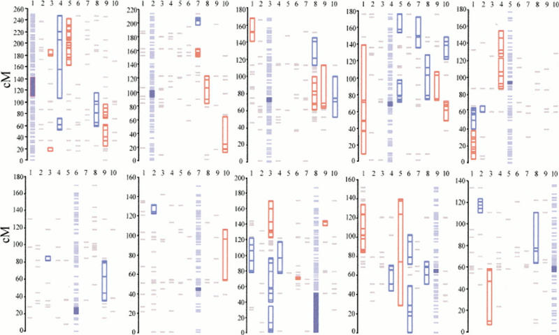
The results of colinearity tests. For each panel, the 10 columns represent the 10 chromosomes. The standard chromosome is shown in light blue, with the centromere in royal blue; the vertical axis represents the centimorgan location on the standard chromosome. Significant colinearities between the standard and tester chromosome are shown on the tester chromosomes in either red (P < 0.005) or dark blue (P < 0.05). (Gray lines) Cross-hybridizing markers that do not comprise significant colinear regions.

Table 2.

Maize Chromosome Pairs with Significant Colinear Runs

Chromosome	P value	Symmetrya	Referenceb
1–3	<0.005	S	none
1–4	<0.005	S	none
1–5	<0.005	S	Helentjaris et al. 1988; Wilson et al. 1999
			Moore et al. 1995b; Gale and Devos 1998a
1–8	<0.05	S	none
1–9	<0.005	S	Helentjaris et al. 1988; Wilson et al. 1999
			Moore et al. 1995b; Gale and Devos 1998a
2–5	<0.05	A	none
2–7	<0.005	S	Helentjaris et al. 1988; Ahn and Tanksley 1993; Moore et al. 1995b; Gale and Devos 1998a; Wilson et al. 1999
2–8	<0.005	A	none
2–10	<0.005	S	Helentjaris et al. 1988; Ahn and Tanksley 1993; Moore et al. 1995b; Gale and Devos 1998a; Wilson et al. 1999
3–6	<0.05	A	none
3–8	<0.005	S	Helentjaris et al. 1988; Ahn and Tanksley 1993; Moore et al. 1995b; Gale and Devos 1998a; Wilson et al. 1999
3–9	<0.005	A	none
3–10	<0.005	S	Moore et al. 1995b; Gale and Devos 1998a
4–5	<0.005	S	Moore et al. 1995b; Gale and Devos 1998a; Wilson et al. 1999
4–7	<0.05	A	Moore et al. 1995b
4–8	<0.05	S	none
4–9	<0.005	A	none
4–10	<0.005	A	none
5–9	<0.005	A	none
6–8	<0.005	A	Helentjaris et al. 1988; Moore et al. 1995b; Gale and Devos 1998a; Wilson et al. 1999
6–9	<0.05	S	Moore et al. 1995b; Gale and Devos 1998a; Wilson et al. 1999
7–10	<0.005	A	none
8–8	<0.005	—	none
8–9	<0.005	S	none
8–10	<0.05	A	none

^aDenotes whether run is symmetric (S) or asymmetric (A). 

^bReferences that discuss chromosomal duplications between the chromosomal pair; includes chromosomal pairs that were explicitly defined as duplicated in text or figures. 

Thirty-eight of the 52 (73.1%) colinear runs were bidirectional, or symmetric. Colinear runs were deemed symmetric if they were detected in both directions and the centimorgan location overlapped in both directions. Chromosomes 1 and 5 provide examples of symmetrical runs, because significant associations were detected when either chromosome was used as the standard (Fig. 4). When chromosome 5 was the standard, one of the significant runs was located from 5.1 to 37.3 cM on chromosome 5 and from 202.1 to 241.3 cM on chromosome 1. Symmetry was evident because the centimorgan location changed little when chromosome 1 was the standard—that is, 5.1–39.4 cM on chromosome 5 and 205.2–241.3 cM on chromosome 1 (Table 1).

The remaining 14 of 52 (26.9%) colinear runs were unidirectional and therefore asymmetric. For example, there was a highly significant association between chromosomes 3 and 9 when chromosome 3 was used as the standard, but there was no association between chromosomes 3 and 9 when chromosome 9 was used as the standard (Table 1; Fig. 4). Asymmetry can be caused by differences in statistical power of the direction of the comparison, but more likely reflect intrachromosomal rearrangements on one of the two chromosomes (Fig. 2).

Some chromosomes have relatively simple patterns of colinearity in which chromosomal regions are associated with one and only one additional chromosome. For example, when chromosome 10 is the standard, the ≈10–60-cM region of chromosome 10 is associated only with chromosome 3; the ≈60–110-cM region of chromosome 10 is associated only with chromosome 8; and the ≈110–125-cM region of chromosome 10 is associated only with chromosome 2 (Fig. 4). This apparent one-to-one correspondence does not hold for most chromosomes. For example, when chromosome 3 is the standard, the ≈60–100-cM region of chromosome 3 shares colinearity with chromosomes 8, 9, and 10. This complex pattern of association is difficult to interpret (see Discussion) but may indicate that the ≈60–100-cM region of chromosome 3 is triplicated or even quadruplicated. Chromosomes 1, 4, 8, and 9 have similarly complex patterns of colinearity.

Colinearity tests were also applied to detect intrachromosomal colinearities, based on markers that cross-hybridize to two different positions within the same chromosome. Only one significant intrachromosomal colinearity was detected, on chromosome 8 (P = 0.0042; Table 1). Thus, there continues to be little evidence of extensive intrachromosomal duplication in maize (Helentjaris et al. 1988).

DISCUSSION

Maize Chromosomal Homology and Comparative Maps of the Grasses

Comparative maps of the grasses recognize that the maize genome contains extensive regions of chromosomal duplication. The colinearity test identified all but one of the previously identified homologous regions (Ahn and Tanksley 1993; Ahn et al. 1993; Moore et al. 1995b; Devos and Gale 1997; Gale and Devos 1998a, 1998b; Wilson et al. 1999), including a region of disputed homology between chromosomes 3 and 10 (Wilson et al. 1999) (Table 2). The lone exception is a potential chromosomal duplication between chromosomes 2 and 4 that was mentioned in one study (Helentjaris et al. 1988) but remains unverified. Thus, the colinearity tests corroborate previously identified regions of chromosomal homology. However, the tests detect significant colinearity between many additional chromosomal pairs (Table 2), and this is true regardless of significance level (P ≤ 0.05 or P ≤ 0.005), metric (d, ss, var, or pr) and error allowance (0.0 or 2.0 cM). Overall, colinearity tests indicate that chromosomal homology in maize is much more widespread than previously documented.

On one level, the differences between comparative mapping studies and this study are not surprising, because the data differ. Comparative maps examine a subset of genetic markers that hybridize to multiple grass species, and this study is based on more markers, many of which hybridize only to maize. On another level, however, the discrepancy between studies is disconcerting, because colinearity tests indicate that the complexity of maize chromosomal relationships have been underestimated by the comparative mapping literature. Such underestimation can lead to overly simplistic conclusions about synteny, chromosomal homology, and grass genome evolution. For example, cereal genomes are commonly represented in a circle format that has been used as a basis for inferring genome evolution (Moore et al. 1995a; Devos and Gale 1997; Gale and Devos 1998a, 1998b). Yet, less than half of the colinear chromosomal pairs detected in this study are represented in the circle (Fig. 5). Thus, inferences about maize genome organization and evolution based on this circle are inaccurate.

Figure 5.

A schematic representing maize homologies inferred from grass comparative maps and the colinearity test. (light and dark gray arcs) Maize chromosomes as often represented in grass comparative maps (Devos and Gale 1997; Gale and Devos 1998a, 1998b; Moore et al. 1995b), with chromosome numbers given. (overlap between chromosomes) Homologies detected by comparative mapping and also by the colinearity test. (black arrows) Additional interchromosomal colinearities detected by the colinearity test.

The discrepancies between this study and the comparative map literature become even more notable when one considers the conservative nature of colinearity results. The results are conservative for four reasons. First, the results are based on the UMC98 map, but the UMC98 map, like most other genetic maps, is based on low-copy markers that do not cross-hybridize extensively among chromosomes. Thus, the data are inherently biased against documenting duplicated regions. Second, the test uses colinearity as an indicator of homology rather than the less stringent criterion of synteny. Third, the colinearity tests examine nonoverlapping runs, precluding detection of significant subruns within longer, nonsignificant runs. The use of non-overlapping runs can only underestimate the true number of significant runs. Finally, with an error allowance of 2.0 cM, the test does not detect any significant colinear runs of less than three markers, indicating that it is difficult to distinguish between statistical noise and colinear regions containing few markers. Altogether, there is likely more colinearity, and hence more homology, among maize chromosomes than documented here.

The Organization and Evolution of the Maize Genome

The extent and pattern of colinearity can be used to better understand the organization and evolution of the maize genome. For example, one can calculate the proportion of the maize genome that is present in at least two copies. At the Bonferroni-corrected level of significance, 129.1 cM of the 249.2-cM length of chromosome 1 is colinear with at least one other chromosome (Fig. 4), indicating that 51.8% of chromosome 1 is duplicated. Expanding this calculation to all 10 chromosomes, the total duplicated proportion of the genome is 44.2% and 69.5% at the P ≤ 0.005 and P ≤0.05 significance levels, respectively. However, these proportions fail to account for the fact that markers at the end of colinear runs may not represent the ends of duplicated segments, and hence duplicated segments are longer than colinear runs. Using the correction of Nadeau and Taylor (equation 2 in Nadeau and Taylor 1984) and assuming that a duplicated segment is either centered in the same map position as the colinear run or anchored at the end of the chromosome, the estimated duplicated proportion of the genome increases to 60.1% and 82.0% at the two significance levels. These proportions still do not correct for the fact that some duplicated segments remain undetected, so the true duplicated proportion of the genome is even higher. Nonetheless, greater than half of the maize genome remains duplicated in chromosomal segments of sufficient size to be detected by marker colinearity, a result consistent with the observation that 72% of rice single-copy markers are duplicated in maize (Ahn and Tanksley 1993).

The number of colinear runs also provides insight into the number of chromosomal rearrangements. Using a variation of published methods (Nadeau and Taylor 1984; Seoighe and Wolfe 1998) and assuming all chromosomal duplications resulted from the tetraploid event, one can estimate the number of chromosomal rearrangements as

where C_S is the number of symmetric (bidirectional) colinear runs, C_Ais the number of asymmetric and intrachromosomal colinear runs, and N₀ is the number of chromosomes originally present in the tetraploid. Briefly, this equation holds because the tetraploid originally had N₀/2 pairs of symmetric colinear runs, each reciprocal translocation event contributed two additional pairs of symmetric colinear runs, and each asymmetric pair represents at least one additional intra- or interchromosomal disruption of linkage. Assuming that the tetraploid initially had 10 chromosomes, this equation yields

rearrangements since the maize tetraploid event. If rearrangements occurred since the tetraploid event ≈11–16 million years ago (Gaut and Doebley 1997), the rate of chromosomal rearrangement has been ≈1.3–1.9 rearrangements per million years. This rate is higher than that of yeast (≈0.7–1.0 reciprocal translocations per million years; Seoighe and Wolfe 1998) and a broad array of mammals (≈0.05–0.9 synteny disruptions per million years; Ehrlich et al. 1997) but similar to rates estimated for diploid cotton species (1.4–2.8 rearrangements per million years; Brubaker et al. 1999).

The estimated rearrangement rate is subject to several sources of error. One source of error is the assumption that rearrangements have occurred since the tetraploid event. This assumption is valid only if the diploid progenitors of maize did not themselves contain duplicated chromosomal regions. Yet, there are at least two reasons to suggest that the diploid progenitors of maize did, in fact, contain duplicated regions. The first reason is that the complex pattern of colinearity—in which one region of a maize chromosome shares colinearity with several different chromosomes (Fig. 4)—suggests that much of the maize genome is multicopy. The multicopy proportion of the genome can be estimated, just as the duplicated proportion of the genome was estimated (see above). With this approach, 8.1% of the genome is multicopy at the P ≤ 0.005 significance level, and 23.2% of the genome is multicopy at the P ≤ 0.05 level. With the Nadeau and Taylor correction (25), these numbers increase to 12.6% and 34.8%. Thus, roughly one-tenth to one-third of the maize genome is multicopy. This is not the first study to suggest that maize genomic regions are triplicated (Helentjaris et al. 1988) or quadruplicated (Wilson et al. 1999), but these results differ by suggesting such regions are common. Multicopy regions can be produced by a tetraploid event between diploid progenitors that contain duplicated regions (Wilson et al. 1999).

The second reason is that small, streamlined genomes such as those of rice and Arabidopsis contain duplicated regions. For example, DNA sequence of Arabidopsis chromosomes 2 and 4 (Lin et al. 1999; Mayer et al. 1999) suggest that 10–20% of low-copy sequences lie within duplicated chromosomal regions (Mayer et al. 1999). More recent studies suggest that a far greater amount of the Arabidopsis genome is duplicated (Blanc et al. 2000). Given the prevalence of multicopy regions in maize and recent information about Arabidopsis, it seems likely that the two diploid progenitors of maize contained extensive duplications.

It is difficult to assess the effect of these duplications on the estimated rate of chromosomal rearrangement in maize. On the one hand, this study has probably underestimated the number of rearrangements, due to conservative assumptions. On the other hand, rearrangements could have occurred in the diploid progenitors, far before the tetraploid event, and thus the rate of rearrangement could be overestimated. In the end, more accurate inferences about rates of chromosomal rearrangement and the extent of multicopy regions will require additional data, such as detailed physical maps, extensive DNA sequence data, or genetic maps based on moderate-copy (as opposed to low-copy) markers. Nonetheless, this work provides a rough estimate of the rate of chromosomal rearrangement in the maize genome, and it also has shown that the maize genome has a complex organization typified by a substantial proportion of multicopy regions.

Two important questions remain. First, what mechanisms have acted to disrupt colinearity in the maize genome? Asymmetric colinearity between chromosomes—for example, asymmetry between chromosomes 3 and 9 (Fig. 4)—could be caused by small rearrangements on one of the two chromosomes, perhaps rearrangements similar to those found in microsyntenic comparisons between grasses (Tikhonov et al. 1999; Tarchini et al. 2000; Bennetzen 2000). Nevertheless, the pattern of colinearity suggests that large chromosomal segments have been translocated, but the mechanisms underlying translocation are presently unclear. Second, the extent of chromosomal duplication raises questions about functional differentiation of duplicated genes. More specifically, what proportion of duplicated genes is lost and what proportion remains functional? This question has received much attention in the evolution literature. For example, theoretical models predict that most duplicated genes will be lost (Nei and Roychoudhury 1973; Takahata and Maruyama 1979; Walsh 1995), but empirical studies suggest more duplicate genes retain function than predicted by theory (Force et al. 1999). Alternative fates for duplicated genes include retention of original function (Ohno 1970), evolution of new or altered expression patterns (Force et al. 1999; Galitski et al. 1999; Lynch and Force 2000), and development of new function (Ohno 1970; Kimura and Ohta 1974). Additional insight into this question requires detailed functional studies of duplicate gene pairs. Note, however, that maize could be a useful system for studying on a broad scale the evolutionary fate of duplicated genes.

The Colinearity Test

Inferences about the maize genome have been based on the colinearity test, which has both advantages and disadvantages. One advantage is that the method requires few assumptions about either genome or marker evolution. Another advantage is objectivity, in that the method does not rely on an ad hoc number of markers to ascertain evidence for chromosomal duplications. A third advantage is that the method uses both centimorgan distances and the number of markers in a run as criteria to evaluate colinearity, although physical rather than genetic distances are more desirable when available. The disadvantages include a potential lack of statistical power, but the fact that the method identifies all but one of the duplications noted in comparative maps suggests it is reasonably powerful. A second weakness is the emphasis on nonoverlapping runs, which could make the method overly conservative.

The general applicability of the colinearity test has yet to be determined, but a similar approach can be applied to other mapped plant genomes that contain extensive chromosomal duplications, such as soybean (Grant et al. 2000), cotton (Brubaker et al. 1999), and Brassica oleracea (Lan et al. 2000). The approach can also be applied across species—for example, a rice chromosome could be used as a standard to compare with all 10 maize chromosomes. Note that the availability of full genome sequences and dense genetic maps does not obviate the need for objective statistical approaches to detect colinear regions. For example, Grant et al. (2000) used a similar but less developed approach to document synteny between Arabidopsis genome sequence and three soybean linkage groups.

Conclusions

The current evolutionary paradigm for grasses, based on comparative map data, asserts that: (1) Gross chromosomal organization has remained largely conserved during 60 million years of grass evolution, (2) 30 rice linkage blocks adequately represent extant grass genomes, and (3) homologous blocks will prove useful for predicting the position of genes conferring key agronomic traits (Devos and Gale 2000). The present study suggests that this paradigm needs to be modified somewhat for maize. First, gross chromosomal organization in maize has changed substantially as a result of duplication and rearrangement, and the time frame for many of these changes is relatively recent (≈11–16 million years ago; Gaut and Doebley 1997; Gaut et al. 2000). Second, the extent of multicopy regions within the maize genome suggests that accurate recognition of block homologies between maize and other grasses may be a more daunting task than previously appreciated.

The question remains as to the best way to unravel grass genome relationships, particularly given the complexity of the maize genome. At present, two separate and sometimes complementary approaches are used to study grass genomes. The first is comparative mapping. Despite the limitations of marker-based maps (Bennetzen 2000), marker-based mapping is still the most accessible way to gain a broad overview of whole-genome (or nearly whole-genome) organization. However, comparative maps often ignore species-specific data in favor of cross-species markers. A useful and efficient alternative may be to focus first on chromosomal relationships within a species—as I have done here in maize—and then to build within-species information into cross-species comparisons. With the exception of maize, it is possible that this “within-species first” approach may not yield surprisingly different results from current grass comparative maps. At the very least, however, a within-species first approach will use existing map data more efficiently. The second approach used to study grass genomes is the microsynteny, or DNA sequencing, approach (for review, see Bennetzen 2000). This approach is invaluable because it provides detailed insights into rearrangement at the molecular level. The corresponding drawback is that microsynteny studies fail to provide a whole-genome view. Until whole-genome sequences and physical maps are available from multiple grass species, additional analyses of marker-based maps may be the best source for additional insights into grass genome organization and evolution.

REFERENCES

- Ahn S, Tanksley SD. Comparative linkage maps of the rice and maize genomes. Proc Natl Acad Sci. 1993;90:7980–7984. doi: 10.1073/pnas.90.17.7980. [DOI] [PMC free article] [PubMed] [Google Scholar]
- Ahn S, Anderson JA, Sorrells ME, Tanksley SD. Homoeologous relationships of rice, wheat and maize chromosomes. Mol Gen Genet. 1993;241:483–490. doi: 10.1007/BF00279889. [DOI] [PubMed] [Google Scholar]
- Anderson E. What is Zea mays? A report of progress. Chron Bot. 1945;9:88–92. [Google Scholar]
- Bennetzen JL. Comparative sequence analysis of plant nuclear genomes: Microcolinearity and its many exceptions. Plant Cell. 2000;12:1021–1029. doi: 10.1105/tpc.12.7.1021. [DOI] [PMC free article] [PubMed] [Google Scholar]
- Bennetzen JL, Freeling M. Grasses as a single genetic system—Genome composition, colinearity and compatibility. Trends Genet. 1993;9:259–261. doi: 10.1016/0168-9525(93)90001-x. [DOI] [PubMed] [Google Scholar]
- ————— The unified grass genome: Synergy in synteny. Genome Res. 1997;7:301–306. doi: 10.1101/gr.7.4.301. [DOI] [PubMed] [Google Scholar]
- Blanc G, Barakat A, Guyot R, Cooke R, Delseny M. Extensive duplication and reshuffling in the Arabidopsis genome. Plant Cell. 2000;12:1093–1102. doi: 10.1105/tpc.12.7.1093. [DOI] [PMC free article] [PubMed] [Google Scholar]
- Brubaker CL, Paterson AH, Wendel JF. Comparative genetic mapping of allotetraploid cotton and its diploid progenitors. Genome. 1999;42:184–203. [Google Scholar]
- Davis GL, McMullen MD, Baysdorfer C, Musket T, Grant D, Staebell M, Xu G, Polacco M, Koster L, Melia-Hancock S, et al. A maize map standard with sequenced core markers, grass genome reference points and 932 expressed sequence tagged sites (ESTs) in a 1736-locus map. Genetics. 1999;152:1137–1172. doi: 10.1093/genetics/152.3.1137. [DOI] [PMC free article] [PubMed] [Google Scholar]
- Devos KM, Gale MD. Comparative genetics in the grasses. Plant Mol Biol. 1997;35:3–15. [PubMed] [Google Scholar]
- ————— Genome relationships: The grass model in current research. Plant Cell. 2000;12:637–646. doi: 10.1105/tpc.12.5.637. [DOI] [PMC free article] [PubMed] [Google Scholar]
- Ehrlich J, Sankoff D, Nadeau JH. Synteny conservation and chromosome rearrangements during mammalian evolution. Genetics. 1997;147:289–296. doi: 10.1093/genetics/147.1.289. [DOI] [PMC free article] [PubMed] [Google Scholar]
- Force A, Lynch M, Pickett FB, Amores A, Yan YL, Postlethwait J. Preservation of duplicate genes by complementary degenerative mutations. Genetics. 1999;151:1531–1545. doi: 10.1093/genetics/151.4.1531. [DOI] [PMC free article] [PubMed] [Google Scholar]
- Gale MD, Devos KM. Comparative genetics in the grasses. Proc Natl Acad Sci. 1998a;95:1971–1974. doi: 10.1073/pnas.95.5.1971. [DOI] [PMC free article] [PubMed] [Google Scholar]
- ————— Plant comparative genetics after 10 years. Science. 1998b;282:65–659. doi: 10.1126/science.282.5389.656. [DOI] [PubMed] [Google Scholar]
- Galitski T, Saldanha AJ, Styles CA, Lander ES, Fink GR. Ploidy regulation of gene expression. Science. 1999;285:251–254. doi: 10.1126/science.285.5425.251. [DOI] [PubMed] [Google Scholar]
- Gaut BS, Doebley JF. DNA sequence evidence for the segmental allotetraploid origin of maize. Proc Natl Acad Sci. 1997;94:6809–6814. doi: 10.1073/pnas.94.13.6809. [DOI] [PMC free article] [PubMed] [Google Scholar]
- Gaut BS, Le Thierry d'Ennequin M, Peek AS, Sawkins MC. Maize as a model for the evolution of plant nuclear genomes. Proc Natl Acad Sci. 2000;97:7008–7015. doi: 10.1073/pnas.97.13.7008. [DOI] [PMC free article] [PubMed] [Google Scholar]
- Goodman MM, Stuber CW, Newton K, Weissinger HH. Linkage relationships of 19 enzyme loci in maize. Genetics. 1980;96:697–710. doi: 10.1093/genetics/96.3.697. [DOI] [PMC free article] [PubMed] [Google Scholar]
- Grant D, Cregan P, Shoemaker RC. Genome organization in dicots: Genome duplication in Arabidopsis and synteny between soybean and Arabidopsis. Proc Natl Acad Sci. 2000;97:4168–4173. doi: 10.1073/pnas.070430597. [DOI] [PMC free article] [PubMed] [Google Scholar]
- Helentjaris T, Weber D, Wright S. Identification of the genomic locations of duplicate nucleotide sequences in maize by analysis of restriction fragment length polymorphism. Genetics. 1988;118:353–363. doi: 10.1093/genetics/118.2.353. [DOI] [PMC free article] [PubMed] [Google Scholar]
- Kimura M, Ohta T. On some principles governing molecular evolution. Proc Natl Acad Sci. 1974;71:2848–2852. doi: 10.1073/pnas.71.7.2848. [DOI] [PMC free article] [PubMed] [Google Scholar]
- Lan TH, DelMonte TA, Reischmann KP, Hyman J, Kowalski SP, McFerson J, Kresovich S, Paterson AH. An EST-enriched comparative map of Brassica oleracea and Arabidopsis thaliana. Genome Res. 2000;10:776–788. doi: 10.1101/gr.10.6.776. [DOI] [PMC free article] [PubMed] [Google Scholar]
- Leister D, Kurth J, Laurie DA, Yano M, Sasaki T, Devos K, Graner A, Schulze-Lefert P. Rapid reorganization of resistance gene homologues in cereal genomes. Proc Natl Acad Sci. 1998;95:370–375. doi: 10.1073/pnas.95.1.370. [DOI] [PMC free article] [PubMed] [Google Scholar]
- Lin XY, Kaul SS, Rounsley S, Shea TP, Benito MI, Town CD, Fujii CY, Mason T, Bowman CL, Barnstead M, et al. Sequence and analysis of chromosome 2 of the plant Arabidopsis thaliana. Nature. 1999;402:761–768. doi: 10.1038/45471. [DOI] [PubMed] [Google Scholar]
- Lynch M, Force A. The probability of duplicate gene preservation by subfunctionalization. Genetics. 2000;154:459–473. doi: 10.1093/genetics/154.1.459. [DOI] [PMC free article] [PubMed] [Google Scholar]
- Mayer K, Schuller C, Wambutt R, Murphy G, Volckaert G, Pohl T, Dusterhoft A, Stiekema W, Entian KD, Terryn N, et al. Sequence and analysis of chromosome 4 of the plant Arabidopsis thaliana. Nature. 1999;402:769–777. doi: 10.1038/47134. [DOI] [PubMed] [Google Scholar]
- McClintock B. A cytological demonstration of the location of an interchange between two non-homologous chromosomes of Zea mays. Proc Natl Acad Sci. 1930;16:791–796. doi: 10.1073/pnas.16.12.791. [DOI] [PMC free article] [PubMed] [Google Scholar]
- ————— The association of non-homologous parts of chromosomes in the mid-prophase of meiosis in Zea mays. Z Zellforsch Mikrosk Anat. 1933;19:191–237. [Google Scholar]
- McMillin DE, Scandalios JG. Duplicated cytosolic malate dehydrogenase genes in Zea mays. Proc Natl Acad Sci. 1980;77:4866–4870. doi: 10.1073/pnas.77.8.4866. [DOI] [PMC free article] [PubMed] [Google Scholar]
- Moore G, Devos KM, Wang Z, Gale MD. Cereal genome evolution—Grasses, line up and form a circle. Curr Biol. 1995a;5:737–739. doi: 10.1016/s0960-9822(95)00148-5. [DOI] [PubMed] [Google Scholar]
- ————— Grasses, line up and form a circle. Curr Biol. 1995b;5:737–739. doi: 10.1016/s0960-9822(95)00148-5. [DOI] [PubMed] [Google Scholar]
- Nadeau JH, Taylor BA. Lengths of chromosomal segments conserved since divergence of mouse and man. Proc Natl Acad Sci. 1984;81:814–818. doi: 10.1073/pnas.81.3.814. [DOI] [PMC free article] [PubMed] [Google Scholar]
- Nei M, Roychoudhury AK. Probability of fixation of nonfunctional genes at duplicate loci. Am Nat. 1973;107:362–372. [Google Scholar]
- Ohno S. Evolution by gene duplication. Heidelberg: Springer-Verlag; 1970. [Google Scholar]
- Passarge E, Horsthemke B, Farber RA. Incorrect use of the term synteny. Nat Genet. 1999;23:387. doi: 10.1038/70486. [DOI] [PubMed] [Google Scholar]
- Peng JR, Richards DE, Hartley NM, Murphy GP, Devos KM, Flintham JE, Beales J, Fish LJ, Worland AJ, Pelica F, et al. 'Green revolution' genes encode mutant gibberellin response modulators. Nature. 1999;400:256–261. doi: 10.1038/22307. [DOI] [PubMed] [Google Scholar]
- Rhoades MM. Duplicated genes in maize. Am Nat. 1951;85:105–110. [Google Scholar]
- ————— . The cytogenetics of maize. In: Sprague GF, editor. Corn and corn improvement. New York: Academic Press; 1955. pp. 123–219. [Google Scholar]
- Seoighe C, Wolfe KH. Extent of genomic rearrangement after genome duplication in yeast. Proc Natl Acad Sci. 1998;95:4447–4452. doi: 10.1073/pnas.95.8.4447. [DOI] [PMC free article] [PubMed] [Google Scholar]
- Snope AJ. The relationship of abnormal chromosome 10 to b-chromosomes in maize. Chromosoma. 1967;21:243–349. [Google Scholar]
- Takahata N, Maruyama T. Polymorphism and loss of duplicate gene expression: A theoretical study with application to tetraploid fish. Proc Natl Acad Sci. 1979;76:4521–4525. doi: 10.1073/pnas.76.9.4521. [DOI] [PMC free article] [PubMed] [Google Scholar]
- Tarchini R, Biddle R, Wineland R, Tingey S, Rafalski A. The complete sequence of 340 kb of DNA around the rice adh1-adh2 region reveals interrupted colinearity with maize chromosome 4. Plant Cell. 2000;12:381–391. doi: 10.1105/tpc.12.3.381. [DOI] [PMC free article] [PubMed] [Google Scholar]
- Tikhonov AP, SanMiguel PJ, Nakajima Y, Gorenstein NM, Bennetzen JL, Avramova Z. Colinearity and its exceptions in orthologous adh regions of maize and sorghum. Proc Natl Acad Sci. 1999;96:7409–7414. doi: 10.1073/pnas.96.13.7409. [DOI] [PMC free article] [PubMed] [Google Scholar]
- Ting YC. Duplications and meiotic behavior of the chromosomes in haploid maize (Zea mays L.) Cytologia. 1966;31:324–329. [Google Scholar]
- Walsh JB. How often do duplicated genes evolve new function? Genetics. 1995;139:439–444. doi: 10.1093/genetics/139.1.421. [DOI] [PMC free article] [PubMed] [Google Scholar]
- Wendel JF, Stuber CW, Edwards MD, Goodman MM. Duplicated chromosomal segments in Zea mays L.: Further evidence from Hexokinase isozymes. Theor Appl Genet. 1986;72:178–185. doi: 10.1007/BF00266990. [DOI] [PubMed] [Google Scholar]
- Wendel JF, Stuber CW, Goodman MM, Beckett JB. Duplicated plastid and triplicated cytosolic isozymes of triosphosphate isomerase in maize (Zea mays L.) J Hered. 1989;80:218–228. doi: 10.1093/oxfordjournals.jhered.a110839. [DOI] [PubMed] [Google Scholar]
- Wilson WA, Harrington SE, Woodman WL, Lee M, Sorrells ME, McCouch SR. Inferences on the genome structure of progenitor maize through comparative analysis of rice, maize and the domesticated panicoids. Genetics. 1999;153:453–473. doi: 10.1093/genetics/153.1.453. [DOI] [PMC free article] [PubMed] [Google Scholar]