Epistasis detection on quantitative phenotypes by exhaustive enumeration using GPUs

Abstract

Motivation: In recent years, numerous genome-wide association studies have been conducted to identify genetic makeup that explains phenotypic differences observed in human population. Analytical tests on single loci are readily available and embedded in common genome analysis software toolset. The search for significant epistasis (gene–gene interactions) still poses as a computational challenge for modern day computing systems, due to the large number of hypotheses that have to be tested.

Results: In this article, we present an approach to epistasis detection by exhaustive testing of all possible SNP pairs. The search strategy based on the Hilbert–Schmidt Independence Criterion can help delineate various forms of statistical dependence between the genetic markers and the phenotype. The actual implementation of this search is done on the highly parallelized architecture available on graphics processing units rendering the completion of the full search feasible within a day.

Availability:The program is available at http://www.mpipsykl.mpg.de/epigpuhsic/.

Contact: tony@mpipsykl.mpg.de

1 INTRODUCTION

The field of bioinformatics matures into a stage of development where the common association search of significant univariate single-nucleotide polymorphism (SNP) to a particular phenotype reveals few novel insights in the underlying biological mechanisms involved. New endeavors must be undertaken to address potential higher order interactions existing among genes in view of revealing underlying common mechanisms in more complex diseases. A brute force exhaustive approach currently poses as a computational challenge. In human studies, the number of SNP can be in the order of millions resulting in the number of possible SNP pair combinations in the order of 10¹²–10¹⁴. The number of individuals can likely be in the range of tens of thousands in large study cohorts. Both dimensions will continue to grow as technological advancement continues on its steady incline. Approaches based on search space pruning and exhaustive search have been adopted for the study on gene–gene interactions in genome-wide association studies. Filtering by main effects to create a subset of SNPs on which all possible interactions are tested for, fails to capture high significance pairs with low main effects. Zhang et al. (2008) and the more generalized form demonstrated by Zhang et al. (2009), are based on space search reduction strategy but is limited to homozygous SNPs and the noted speedup factor has not been substantial for large sample size. The most compelling search space pruning method developed by Zhang et al. (2010) has overcome these shortcomings but is limited to tests based on contingency tables where classes on the phenotype exist. As tools involved in collecting data improve, the software and computational strategy employed for the analysis should be refined to accommodate for these changes and should not limit the type of investigation that can be undertaken.

In Kam-Thong et al. (2010), a difference of Pearson's correlation coefficients between binary phenotypes across all possible SNP pairs has been developed. This approach of a difference in correlation coefficients is not only mathematically appealing for its simplicity and from a practical standpoint for the comparative ease with which it can be computed, but is also interesting and appealing from a biological standpoint—it ties up the concepts of epistasis with the evolutionary concept of co-selection of unlinked loci.

This search protocol was implemented on graphics processing units (GPUs) using the available parallel computing capability to reduce the search time by several orders of magnitude compared to single-core CPU-based computation. However, this method is strictly limited to binary phenotypes. When the recorded phenotypes are of quantitative nature, differences of test measures cannot be performed between classes/clusters of datasets as compared to the binary or qualitative phenotype counterparts where classes of subjects preexist. This article aims to present the steps that were taken to overcome this severe limitation and extend this method to quantitative phenotypes.

The proposed search strategy performs an exhaustive search for interaction significance across all SNP pairs against a quantitative phenotype. The method is derived from the Hilbert–Schmidt Independence Criterion (HSIC) developed by Gretton et al. (2005). Furthermore, the implementation is done on commercially available GPUs to reduce the financial costs and search time. The actual timing measure will depend largely on the marker coverage size and computer resource utilized. However, the order of speedup factor is consistently observed throughout.

This article is structured in the following order. It will first extend the correlation difference method developed for binary phenotypes in Kam-Thong et al. (2010) to quantitative phenotypes by demonstrating it as an instance of HSIC. The proposed method is applied on a set of simulated data and a set of real data in the results section. Improved efficiency is measured between the GPU implementation and its CPU counterpart. Validation is determined by a comparison to the significance of the interaction term using linear regression fit.

2 METHODS

2.1 Algorithm derivation

2.1.1 Setting

We assume that we are given a set of n patients with genotypes X and phenotypes Y. Patient i has genotype x_i and phenotype y_i. Each genotype x_i∈IR^m, where m is the number of SNPs. SNP A of patient i is denoted by x_i^A∈{0, 1, 2}.

We further assume that the phenotypes are binary, that is y_i∈{0, 1}. If y_i=1, we refer to patient i as a case, if y_i=0, we refer to this patient as a control. We denote the number of cases by n₁, the number of controls by n₀, such that n≔n₀+n₁.

2.1.2 Correlation coefficient difference method on binary phenotype

The method developed in Kam-Thong et al. (2010) uses the correlation coefficient difference between cases and controls, (1), as an approximation to the significance of the interaction term resulting from the logistic regression on dichotomous phenotypes:

(1)

Here and represent the two SNPs A and B, which have been centered by subtracting their mean and rescaled by dividing them by the standard deviation for each subject class, cases (y_i=1) and controls (y_i=0), respectively.

The reasoning in Kam-Thong et al. (2010) is that SNP pairs (A,B) with the largest difference in correlation between cases and controls are most likely to exhibit an epistatic interaction. The search for these SNP pairs with maximum Δρ(X^(A,B), Y) is performed by exhaustive search by means of a highly efficient graphical processing unit (GPU) implementation. This GPU implementation allows to conduct the search for epistatic interactions on datasets with 100s of individuals and 100 000s of SNPs in less than a day.

However, the formulation in Kam-Thong et al. (2010) suffers from one severe limitation, which is that it only applies to binary phenotypes. In the following, we show how to overcome this problem via the HSIC.

2.1.3 HSIC

The HSIC is a statistical measure of independence of two random variables Gretton et al. (2005). Intuitively, HSIC can be thought of as a squared correlation coefficient between two random variables x and y computed in feature spaces ℱ and 𝒢.

In more detail, let x be a random variable from the domain 𝒳 and y a random variable from the domain 𝒴. Let ℱ and 𝒢 be feature spaces on 𝒳 and 𝒴 with associated kernels k:𝒳×𝒳→ℝ and l:𝒴×𝒴→ℝ. If we draw pairs of samples (x,y) and (x′,y′) from x and y according to a joint probability distribution p_(x,y), then the HSIC can be computed in terms of kernel functions via:

(2)

where E is the expectation operator. The empirical estimator of HSIC for a finite sample of points X and Y from x and y was shown in (Gretton et al., 2005) to be

(3)

where tr is the trace of the products of the matrices, H is a centering matrix (where δ_(i,j)=1 if i=j and δ_(i,j)=0 otherwise) and K and L are the kernel matrices of the two data sets of size n×n, n being the number of observations/individuals of the study. The larger HSIC, the more likely it is that X and Y are not independent from each other.

2.1.4 Difference of correlation of coefficients as an instance of HSIC

As a first step towards generalization to non-binary phenotypes, the difference of correlation between cases and controls in Equation (1) can be expressed as an instance of HSIC.

Theorem 2.1. —

Given two spaces ℱ with kernel k and 𝒢 with kernel l. Let k and l be defined via

(4)

(5)

where ψ(y_i) is defined via:

(6)

Then

(7)

Proof. —

The theorem is shown by the following derivation:

(8)

(9)

(10)

(11)

(12)

(13)

The transition from (8) to (9) follows from the fact that l gives rise to a centered kernel matrix (L=HLH) and equation (3). (10) follows from (9) due to the definition of k, and (12) from (11) due to the definition of l.▪

2.1.5 Generalization of HSIC to quantitative phenotypes

What we learn from Theorem 2.1 is that the difference in correlation of two SNPs A and B on cases and controls is an instance of HSIC for a specific choice of the kernel l. In Kam-Thong et al. (2010), this kernel l is chosen for binary phenotypes, as obvious by its definition in (Equation 6). To generalize the difference in correlation to non-binary phenotypes, we have to choose a kernel for non-binary phenotypes.

If the phenotypes are real numbers, that is y_i∈ℝ we may choose the centered linear kernel (that is, ) as kernel on the centered phenotypes , giving rise to the following criterion for SNP pair interaction.

Definition 2.2 (epiHSIC). —

We define l to be a centered linear kernel on real-valued phenotypes and k as a kernel on SNP pairs as in equation (4). Then

(14)

is a statistical measure of interaction between the SNP pair (A,B) and the real-valued phenotypes Y.

The following lemma follows immediately from the proof of Theorem 2.1 and the definition of epiHSIC:

Lemma 2.3. —

epiHSIC_empirical((X,Y),ℱ,𝒢) can be computed in a runtime which is linear in n by rewriting it as

(15)

(16)

Hence on n patients with m SNPs, an exhaustive computation of epiHSIC statistics for all pairs of SNPs will require a runtime of O(m²n) based on the lemma above. epiHSIC is the instance of HSIC which we implement on GPUs and use in our experiments in what follows.

2.2 Relationship between HSIC and linear regression

Before moving to the GPU implementation, we theoretically investigate why the proposed HSIC can be used as an approximation to the linear regression coefficient estimates that are often used in statistical genetics to quantify the impact of variables on the phenotype. For this purpose, we examine the derivation of estimates using the least squares regression method and compare it to HSIC.

Starting with the linear function of the simplest form,

(17)

where ψ:ℝ→ℝ and ϕ:ℝ→ℝ. The residuals, R, of the estimated mapped output ψ(ŷ) and observed mapped output ψ(y) can then be squared,

(18)

The minimal residual term can be solved by partial differentiations on coefficients a, b to yield optimal parametric estimates. Differentiating R² by parameter a and setting it to zero,

(19a)

(19b)

Similarly, for coefficient b,

(20a)

(20b)

Combining the two equations in matrix form (sums are implied over i) and solving for coefficient b,

(21)

(22)

(23)

(24)

where the last line follows from the definition of HSIC if we assume ϕ and ψ to be the feature maps into space ℱ and 𝒢, respectively, and if both ϕ and ψ rescale the data x and y to zero mean and unit variance.

This shows that the mean estimated parameter b is proportional to HSIC scaled by the ratio of the standard deviations of the output (phenotype ψ(y)) and the input (SNP–SNP interaction ϕ(x)=x^Ax^B). The variance of the phenotype for each pair tested can only vary on the basis of missing subjects from one SNP pair to another due to incomplete genotyping. Moreover, the variance of the input does not change significantly from one pair to another in practice. For example in the dosage encoding, the minor allele is counted and the product of two SNPs can only take on discrete values from the finite set 0, 1, 2, 4. Consequently, high HSIC value should lead to an estimated parametric coefficient further away from null which also implicates lower residuals in the fit. Based on this relationship, the estimated parameters across all SNP pairs should be correlated to HSIC if the standard deviations of the phenotype and the SNP pairs are confined within a certain range.

2.3 Implementation on GPU

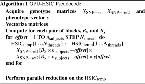
The GPU provides a massively parallel computational environment in which the exhaustive SNP pairs search can be conducted in a time efficient manner. Currently, there are several hundred of arithmetic logic units (ALUs) on a single GPU, which is the most appealing aspect over conventional CPU based computing. The Compute Unified Device Architecture (CUDA) C programming language developed by NVIDIA is an extension to the C language specifically designed to facilitate general-purpose GPU (GPGPU) computing and harness the computational power of GPUs built with NVIDIA's CUDA Architecture. Communication latency related to memory transfer poses as the main performance bottleneck in GPGPU computing. It is important to supply the graphic device with ample amount of input data to keep all its cores busy in view of achieving maximal performance. Accessing memory within the GPU and waiting for all threads to synchronize before carrying on subsequent calculations are also another source of slowdown. As HSIC between each SNP pair and the phenotype can be tabulated independently, this can take full advantage of GPU.

To perform HSIC between every possible SNP pair and the quantitative phenotype, two genotype matrices (X_SNP−set1 and X_SNP−set2), matrices with column vectors of subset number of SNPs, and the phenotype vector y_Phenotype are passed on to the GPU. The reason the genotype data must be partitioned is due to physical memory limitation on the device. The genotype X_SNP−set1X_SNP−set2^T matrix cross product guarantees that the product of all possible pairs of SNPs across all individuals will be computed. At the heart of GPU computing is the ability to keep computation on multiple threads running in parallel. Threads are grouped in blocks and there is a limit of the number threads that can be used per block, N_threads. In order to perform computation on vectors greater than N_threads, the use of a combination of threads and blocks is necessary. There is an inherent trade-off between the number of blocks versus the size of the blocks. The overall process consists of the computation of multiplications and three sets of summations which can take full advantage of the GPU environment. The first sum is used to tabulate the mean, second to find the standard deviation and lastly, the HSIC is computed using the mean and standard deviation stored in shared memory. The speedup factor is accomplished by performing running sums in groups of N_threads, termed warp, in the single instruction, multiple data (SIMD) format in GPU before collapsing it back to a single scalar value using conventional parallel reduction algorithm.

3 RESULTS

3.1 Experimental data

The method is first tested on simulated data followed by real data obtained from a depression study using Hamilton Depression Rating Scale as the quantitative phenotype for each individual. Although the dosage model was chosen for the experiments, the genotype data can in fact also be coded using a dominant, recessive or heterozygous model based coding.

3.2 Hardware and software setup

The hardware used in the experimental setup consists of two pairs of commercially available NVIDIA GTX295 (Santa Clara, CA, USA) CUDA-enabled NVIDIA graphic cards running on an Intel Core i7 920 with 2.67 GHz (Santa Clara, CA, USA) central processing unit host (CPU) using 12 GB of DDR3 RAM (Corsair Inc., Fremont, CA, USA). The software program is implemented in R (version 2.9.2; R Development Core Team, 2010) with the gputools package beta version 0.1–4 installed (Buckner et al., 2010, http://cran.r-project.org/web/packages/gputools), in which the function has been modified to be passed two genotype input matrices and one phenotype output vector.

A R package, GenABEL version 1.6-4 (http://cran.r-project.org/web/packages/GenABEL/), is used for data compression when the genotype is read into R as a single file. Each element is represented by two bits covering the dosage model encoding 0, 1, 2. When elements are recorded in floating-point numbers as in genotypic probabilities, this step is bypassed by partitioning into smaller size files where the local memory limitation would not be of a constraint. At the writing out stage, when a P-value threshold is chosen to filter the results that only show promises of true multiple test wise significance, it will unlikely surpass the disk storage limitation. If it is desired to store results covering a greater range, R permits for writing out in compressed formats.

3.3 Simulation data

3.3.1 Validation

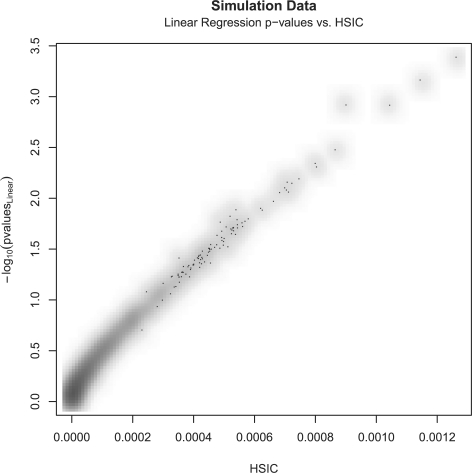
For the purpose of validating the method, data are simulated using a normally distributed output phenotype (mean = 0 and standard deviation = 1) and genotype SNP value in {0, 1, 2} encoding. The number of individuals is set to 10 000 subjects and 50 SNPs, resulting in 1225 unique SNP pairs. These SNPs are simulated in Hardy–Weinberg equilibrium (P=0.05). Testing for the significance of the interaction SNP pair with respect to the quantitative phenotype, a standard linear regression on the full rank model including main effects is performed (ψ(y)=α+βx^A+γx^B+δx^Ax^B), where the significance of the coefficient δ is compared to the HSIC realization derived for quantitative phenotype in Section 2.1. A total of 1225 pairs are compared; this is a relatively small and unrealistic number of pairs but it serves only to demonstrate the validity of the method. As illustrated in Figure 1, the HSIC is compared against the −log₁₀ of the P-value obtained from the likelihood ratio test comparing the regression models without and with the interaction term. The r² is noted to be 0.9764, indicating that the HSIC is strongly correlated with the significance of the interaction term sought after.

Fig. 1.

−log₁₀ Linear regression P-values versus the HSIC for 50 SNPs (1225 pairs) — r²=0.9764.

3.3.2 Time performance

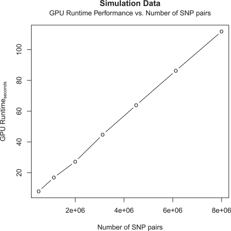
In order to gain an insight on the improved time performance, 10 000 subjects genotyped over 4000 SNPs are artificially simulated. A time comparison is made on the HSIC calculation between a single core CPU and GPU to reveal the advantage of porting the implementation onto GPU. The CPU performance is largely dependent on the technical specifications (clock speed, number of cores and cache memory) and current load on the system. Using a single core on the Intel Core i7 CPU, on average, it can compute the HSIC between the quantitative phenotype and ~800 SNP pairs per second in R. The GPU runtimes with varying number of SNP pairs are plotted in Figure 2. It is observed that GPU runtime varies linearly with the number of SNP pairs tested. The speedup factor relative to a single CPU remains consistent, in the range of ~80–92. The results are detailed in Table 1.

Fig. 2.

GPU Runtime versus the number of SNP pairs in Simulation Data.

Table 1.

Results from the full HSIC model

SNPs	Pairs	Runtime [s]	Interactions [1/s]	Speedup factor versus Single CPU
4000	7 998 000	111.79	71 546.78	89.93
3500	6 123 250	86.27	70 976.10	88.72
3000	4 498 500	63.86	70 444.26	88.06
2500	3 123 750	44.73	69 834.12	87.29
2000	2 000 000	27.16	73 600.88	92.00
1500	1 124 250	16.86	66 669.63	83.34
1000	499 500	7.87	63 476.93	79.35

3.4 Real data—Hamilton Rating Scale

3.4.1 Data

The Hamilton Depression Rating Scale is the standard questionnaire used to assess the severity of a patient's depression. The data is collected from a depression study. More details on the phenotype can be found in Binder et al. (2004) and Ising et al. (2009). There is also a large overlap between the individuals in these two studies and this consideration, all originating from the MARS study. The quantitative phenotype used in this article is the percent change of the scale in week 2 relative to scale tallied in the baseline week 0 for each patient. A total of 491 patients genotyped over 536 750 SNPs is used in this study. The objective of the study is to uncover gene–gene interactions which can help explain the variation in rate of recovery among patients. The goal is to ultimately tailor the treatment for patients having just suffered an episode of depression based on their genetic makeup.

3.4.2 Validation

Linear regression is run on 48 CPU cores to compare against the EpiGPUHSIC method. This comparison is made simply to reveal the current state of the art on GWAS based exhaustive epistasis detection. In order to perform the linear regression on this brute-force approach in a time efficient manner, the use of a newly released software tool, FastEpistasis (http://www.vital-it.ch/software/FastEpistasis), is required. This is an extension of the PLINK (Purcell et al., 2007) epistasis module capable of distributing the work in parallel on multiple CPU cores. Running the proposed method on the GPU requires ~40 h to complete as compared to ~57 h for completion using FastEpistasis on 48 AMD Opteron 6172 2.1 GHz CPU cores (Sunnyvale, CA, USA) with ATLAS BLAS/LAPACK version 3.2.1 (Whaley and Petitet, 2005). It is important here to note that only the first and second stages of FastEpistasis were included, the time required in the third stage for writing out the results given a P-value threshold from the binary files has been neglected, although it can be substantial.

A comparison of the time performance between the two tests is summarized in Table 2. It is noted that EpiGPUHSIC on a single graphic card outperforms FastEpistasis on 48 CPU cores by a factor of 1.4. By taking into account that 48 CPU cores are used, this observation is comparable to the noted speedup factor in Section 3.3.2.

Table 2.

Hamilton Rating Scale—Data and performance summary

HSIC runtime	FastEpistasis runtime
GPU [min]	48 CPUs [min]
2 408.92	3 440.30
(~40 h)	(~57 h)

Checking 536 750 SNPs (1.44×10¹¹ pairs) in 491 subjects. 1 137 450 interactions below a threshold of P<10⁻⁵ are found.

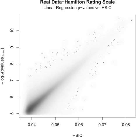
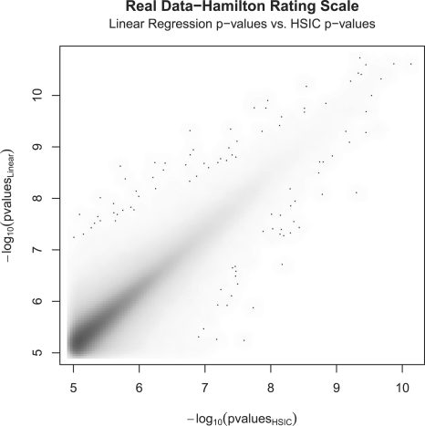
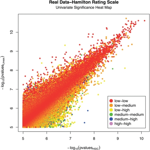
In Figure 3, the HSIC values are plotted against the P-values of the linear regression on the interaction term. Furthermore, it has been shown that the distribution of HSIC is asymptotically approaching normal (Gretton et al., 2005), which in turn allows for significance tests to be performed based on standard statistics. The P-values of the HSIC terms are compared to the P-values of the linear regression on the interaction term (Fig. 4).

Fig. 3.

Overall fit done on the top one million matching pairs. −log₁₀ Linear regression interaction model versus HSIC.

Fig. 4.

Overall fit done on the top one million matching pairs. −log¹⁰ Regression interaction model versus −log₁₀ HSIC P-values.

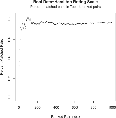
Moreover, in order to verify that no significant number of pairs are left unmatched between the two methods, a percent match moving across the ranked pairs is performed (Fig. 5). The noted behavior further consolidates the fact that the approximation method does hold, as it quickly approaches ~75% matched pairs in the first 1000 ranked pairs between the two methods.

Fig. 5.

Matching pairs capture rate across the first 1000 ranked pairs between the standard linear regression fit and the proposed HSIC method.

Furthermore, to investigate the univariate SNP effect in the quality of the fit between the proposed HSIC method and the linear regression, the P-values of the univariate SNPs are color coded in Figure 6. The P-values of the univariate SNP range from 1 (insignificant) down to 6.2·10⁻⁶. Univariate significances are classified as low (P>0.1), medium (0.01<P≤0.1) and high (P≤0.01). Each pair is classified in one of the six unique possible combinations of univariate significances. The quality of the fit is investigated separately for each univariate significances combination class, see Table 3. As expected, there is an overwhelming amount of low significance univariate SNP. The quality of the fit between the HSIC method and linear regression is tested when the datapoints are segregated into three separate groups of univariate SNP significance. It is noted that the quality of the fit varies inversely to the significance of the univariate SNP. A higher univariate significance will lead to a poorer fit between the two methods. Therefore, the proposed HSIC method is a better approximation to the linear regression when the univariate significance is lower. This observation makes intuitive sense but points out a weakness in the method, as HSIC neglects univariate effects in its assessment.

Fig. 6.

−log₁₀ Linear regression interaction P-values versus −log₁₀ HSIC P-values (−log₁₀ univariate SNP1 P-values of each pair is represented by color scale ranging from insignificant to significant from the red to blue spectrum).

Table 3.

Hamilton Rating Scale-data and performance summary

Univariate xA−xB significances	Number of pairs	Correlation Coefficient HSIC versus Lin. Reg.
Low–low	934 611	0.94
Low–medium	176 099	0.83
Low–high	16 807	0.70
Medium–medium	8239	0.74
Medium–high	1471	0.58
High–high	79	0.56

3.4.3 Top pairs and biological relevance

Table 4 lists the results for the ten SNP pairs showing the strongest interaction with respect to the significance test done on the linear regression. It is very interesting to note that there is an apparent connection between the top pairs as rs11580794, a member of the top pair is located nearby PBX1, whereas rs12910772, a member of the runner-up is very close to MEIS2. In general the PBX and MEIS genes apparently interact in brain development. Furthermore, PBX1 has a function in glucocoticoid signalling, which is an obvious candidate pathway in depression and its treatment (Holsboer, 2008). In addition, we see significant (P=0.0345) evidence for an interaction between the two top pairs, augmenting the hypothesis that there may be a role for the PBX/MEIS system in this phenotype. See Table 5 for all associated genes (within ± 100 kb).

Table 4.

Top ten results from Hamilton-score.

SNP1	SNP2	HSIC		Linear regression
		Value	P-value	SNP1 P-value	SNP2 P-value	Interaction P-value
rs11580794	rs11812623	7.70·10−02	4.42·10−10	0.9601	0.03071	1.87·10−11
rs12910772	rs2338712	8.22·10−02	1.35·10−10	0.3682	0.77860	2.44·10−11
rs13028359	rs2888542	8.24·10−02	7.39·10−11	0.2710	0.83590	2.45·10−11
rs13401572	rs6130852	7.87·10−02	3.58·10−10	0.1360	0.40590	2.54·10−11
rs2105126	rs1885418	7.90·10−02	2.62·10−10	0.2911	0.56040	2.71·10−11
rs861256	rs11864516	7.93·10−02	1.78·10−10	0.4486	0.91110	2.90·10−11
rs6442323	rs13186058	7.74·10−02	2.61·10−10	0.2621	0.66000	3.29·10−11
rs6442323	rs4958287	7.74·10−02	2.61·10−10	0.2621	0.66000	3.29·10−11
rs6442323	rs4958505	7.80·10−02	2.24·10−10	0.2621	0.58860	3.43·10−11
rs7797027	rs1031912	7.87·10−02	2.72·10−10	0.7797	0.85880	3.46·10−11

Bold P-values indicate significance at the 0.05 level.

Table 5.

Physical annotation of the top ten Hamilton-score results

SNP	Position Chr [kb]	Gene	Distance [kb]
rs11580794	1:163 120	PBX1	+40
rs11812623	10:79 860	SNORA71	+60
rs12910772	15:34 960	MEIS2	+10
rs2338712	22:47 210
rs13028359	2:19 940	TTC32	+20
		WDR35	+30
rs2888542	2:37 760	CDC42EP3	−10
rs13401572	2:157 660
rs6130852	20:43 575	SPINT3	0
		WFDC6	+20
		SPINLW1	+30
		WFDC8	+40
		WFDC2	+30
rs2105126	1:80 980
rs1885418	14:95 150	TCL2	−40
rs861256	11:33 700
rs11864516	16:725	NARFL	0
		HAGHL	+5
		CCDC78	−10
		C16orf24	+10
		METRN	+20
		FBXL16	−30
		MSLN	−25
		MPFL	+30
		RPUSD1	+50
rs6442323	3:12 700	RAF1	−20
rs13186058	5:151 311	GLRA1	−30
rs6442323	3:12 700	RAF1	−20
rs4958287	5:151 310	GLRA1	−30
rs6442323	3:12 700	RAF1	−20
rs4958505	5:151 325	GLRA1	−40
rs7797027	7:15 455	FLJ16327	0
rs1031912	15:92 390

In the distance column ‘−’ indicates upstream of the gene, ‘+’ downstream of the gene, a distance of 0 means in the gene.

4 CONCLUSION AND FUTURE WORK

The difference of correlation method for binary phenotypes developed in Kam-Thong et al. (2010) has successfully been extended for quantitative phenotypes. This is accomplished by expressing the test as an instance of HSIC and by making the necessary adjustment on the mapping function applied. By making such an association, we have overcome the strict limitation of Kam-Thong et al. (2010) and unlocked the method to perform various forms of statistical dependence tests between SNP pair interaction and the phenotype. The proposed HSIC realization in this article uses linear kernels since the validity of the results can be easily cross-verified with the outcome of the linear regression fit on the interaction term. While these linear kernels result in HSIC being proportional to Pearson's correlation coefficient, the use of other forms of kernels will be investigated in the near future. They will allow us to extend the framework described here to quantitative phenotypes modelled as time series, images or videos. Another avenue of future research is to implement linear and logistic regressions on GPUs, which is more involved than the GPU implementation of EpiGPUHSIC but provides a direct way of assessing the main effect of individual SNPs when scoring pairs of SNPs for association.

To evaluate the effects of any potential confounding factors, linkage disequilibrium and HSIC scores are tabulated across all possible pairs from 2000 SNPs in chromosome 1 of HapMap phase 3 CEU subjects. A r² of 3.19·10⁻⁵ is noted between the two measures, thus, ruling out any confounding factor due to linkage disequilibrium.

To investigate the potential pitfall of using space-pruning techniques based on main effects, the first 10 000 most significant interaction pairs obtained from a full exhaustive search and their corresponding main effects P-values are analyzed. It shows minimal correlation, r² of 5.17·10⁻⁵ and 2.23·10⁻³ for the first and second SNP of the pairs, respectively. Furthermore, we have adopted the space pruning solutions by retaining the top 10% most significant main effect SNPs and performed an exhaustive search with the remaining 90% SNPs. When these results are compared to the full exhaustive search results, only a small percentage of the findings can be matched, leaving 87% of the pairs in the top 10 000 ranked SNP pairs from the full exhaustive search method unresolved. If we are to further limit the exhaustive search of the top 10% most significant univariate SNPs within its own subset, the matching pairs compared to the ranked significant pairs obtained from the brute force exhaustive drops down to a mere 0.8% for the first 10 000 ranked SNP pairs.

Low correlation between the randomness of any potential additive noise on the output signal with the input signal further favors the proposed HSIC approach. As the signal-to-noise ratio in the output measurements approaches a critical threshold, this method should be more robust as compared to the least squares fitting since the correlation term between the noise and the input will approach zero, thus having no effect in the test. Further investigation needs to be performed.

Furthermore, a multiplicative effect (and) is assumed between the SNPs in each pair. This can be further modified to accommodate for other forms of interaction (multiplicative within and between loci or interaction threshold effects) detailed in (Marchini et al., 2005) and applying other logical operators such as nor, xor, nand. The biological relevance of these models remains to be explored.

Testing millions and billions of epistatic interactions requires correction for multiple hypothesis testing. As Bonferonni correction often results in highly conservative significance thresholds, permutation-based statistical tests such as Zhang et al. (2010) have been proposed in the literature. In future work, we will work on GPU implementations of permutation-based tests of significance for EpiGPUHSIC and related methods.

REFERENCES

- Binder E.B., et al. Polymorphisms in FKBP5 are associated with increased recurrence of depressive episodes and rapid response to antidepressant treatment. Nat. Genet. 2004;36:1319–1325. doi: 10.1038/ng1479. [DOI] [PubMed] [Google Scholar]
- Buckner J., et al. The gputools package enables GPU computing in R. Bioinformatics. 2010;26:134–135. doi: 10.1093/bioinformatics/btp608. [DOI] [PMC free article] [PubMed] [Google Scholar]
- Gretton A., et al. Proceedings of the International Conference on Algorithmic Learning Theory. Singapore: Springer; 2005. Measuring statistical dependence with Hilbert-Schmidt norms; pp. 63–77. [Google Scholar]
- Holsboer F. How can we realize the promise of personalized antidepressant medicines? Nat. Rev. Neurosci. 2008;9:638–646. doi: 10.1038/nrn2453. [DOI] [PubMed] [Google Scholar]
- Ising M., et al. A genomewide association study points to multiple loci that predict antidepressant drug treatment outcome in depression. Arch. Gen. Psychiat. 2009;66:966–975. doi: 10.1001/archgenpsychiatry.2009.95. [DOI] [PMC free article] [PubMed] [Google Scholar]
- Kam-Thong T., et al. Epiblaster - fast exhaustive two-locus epistasis detection strategy using graphical processing units. European J. Hum. Genet. 2010;19:465–471. doi: 10.1038/ejhg.2010.196. [DOI] [PMC free article] [PubMed] [Google Scholar]
- Marchini J., et al. Genome-wide strategies for detecting multiple loci that influence complex diseases. Nat. Genet. 2005;37:413–417. doi: 10.1038/ng1537. [DOI] [PubMed] [Google Scholar]
- Purcell S., et al. Plink: a toolset for whole-genome association and population-based linkage analysis. Am. J. Hum. Genet. 2007;81:559–575. doi: 10.1086/519795. [DOI] [PMC free article] [PubMed] [Google Scholar]
- R, Development Core Team. R: A Language and Environment for Statistical Computing. Vienna, Austria: R Foundation for Statistical Computing; 2010. [Google Scholar]
- Whaley R.C., Petitet A. Minimizing development and maintenance costs in supporting persistently optimized BLAS. Software Pract. Exp. 2005;35:101–121. [Google Scholar]
- Zhang X., et al. Proceeding of the 14th ACM SIGKDD international conference on Knowledge discovery and data mining. Las Vegas, Nevada, USA: ACM; 2008. Fastanova: an efficient algorithm for genome-wide association study; pp. 821–829. [PMC free article] [PubMed] [Google Scholar]
- Zhang X., et al. Proceedings of RECOMB 2009. Tuscon, Arizona, USA: Springer; 2009. COE: A general approach for efficient genome-wide two-locus epistasis test in disease association study; pp. 253–269. [DOI] [PubMed] [Google Scholar]
- Zhang X., et al. TEAM: efficient two-locus epistasis tests in human genome-wide association study. Bioinformatics. 2010;26:i217–i227. doi: 10.1093/bioinformatics/btq186. [DOI] [PMC free article] [PubMed] [Google Scholar]