Identification of metabolic network models from incomplete high-throughput datasets

Abstract

Motivation: High-throughput measurement techniques for metabolism and gene expression provide a wealth of information for the identification of metabolic network models. Yet, missing observations scattered over the dataset restrict the number of effectively available datapoints and make classical regression techniques inaccurate or inapplicable. Thorough exploitation of the data by identification techniques that explicitly cope with missing observations is therefore of major importance.

Results: We develop a maximum-likelihood approach for the estimation of unknown parameters of metabolic network models that relies on the integration of statistical priors to compensate for the missing data. In the context of the linlog metabolic modeling framework, we implement the identification method by an Expectation-Maximization (EM) algorithm and by a simpler direct numerical optimization method. We evaluate performance of our methods by comparison to existing approaches, and show that our EM method provides the best results over a variety of simulated scenarios. We then apply the EM algorithm to a real problem, the identification of a model for the Escherichia coli central carbon metabolism, based on challenging experimental data from the literature. This leads to promising results and allows us to highlight critical identification issues.

Contact: sara.berthoumieux@inria.fr; eugenio.cinquemani@inria.fr

Supplementary information: Supplementary data are available at Bioinformatics online.

1 INTRODUCTION

To further our understanding of the cellular processes shaping the response of microbial cells to changes in their environment requires the study of the interactions between gene expression and metabolism. In recent years high-throughput datasets comprising simultaneous measurements of metabolism (fluxes, metabolite concentrations) and gene expression (protein and mRNA concentrations) have become available (Hardiman et al., 2007; Ishii et al., 2007). These datasets provide a rich store of information for modeling the dynamics of the biochemical reaction systems underlying cellular processes. In particular, they promise to relieve what is currently a bottleneck for modeling in systems biology, obtaining reliable estimates of parameter values in kinetic models (Ashyraliyev et al., 2009; Crampin, 2006).

Notwithstanding these experimental advances, parameter estimation remains a particularly challenging problem, among other things due to incomplete knowledge of the molecular mechanisms, noisy and partial observations, heterogeneous experimental methods and conditions, and the large size of networks (Marucci et al., 2011). As a consequence, the models may not be identifiable, may not generalize to new situations due to overfitting, and nonlinear rate functions may make them cumbersome to analyze. This has led to the proposal of simplified kinetic modeling frameworks, including linlog kinetics (Visser and Heijnen, 2003), loglin kinetics (Hatzimanikatis and Bailey, 1997), power-law kinetics (Savageau, 1976), and more recently, convenience kinetics (Liebermeister and Klipp, 2006).

Linlog models are a particularly interesting choice for modeling metabolism (Heijnen, 2005; Visser and Heijnen, 2003). Simulation studies on the level of both individual enzymatic reactions (Heijnen, 2005) and metabolic networks (Costa et al., 2010; Hadlich et al., 2009; Visser et al., 2004) have shown that they provide reasonable approximations of classical enzymatic rate laws. Moreover, with the help of a recent genome-scale linlog model of yeast metabolism, parametrized using previously-published kinetic models, it has been possible to identify key steps in the network, that is, reactions exerting most control over glucose transport and biomass production (Smallbone et al., 2010).

A major advantage of linlog models is that, when measurements of fluxes, enzyme concentrations and metabolite concentrations are available, the parameter estimation problem reduces to multiple linear regression (Nikerel et al., 2006). Power-law models, up to a logarithmic transformation, and loglin models also have this convenient property. However, the performance of regression approaches quickly degrades in the presence of missing data, as is often the case in high-throughput datasets due to experimental limitations or instrument failures.

In order to deal with this problem, we propose in this article a maximum-likelihood method for the identification of linlog models of metabolism from incomplete datasets. The specific contributions of the paper are 2-fold. On the theoretical side, we develop a method for the optimization of the likelihood based on Expectation Maximization (EM) (Dempster et al., 1977). The method is constructed for linlog models, but is more generally applicable to other approximate kinetic models whose identification can be formulated as a regression problem. In particular, we derive analytical expressions for the expectation step that are well-suited for numerical maximization. This guarantees the applicability of the approach even when modeling large networks. We show by means of simulation experiments on synthetic data that our approach outperforms both regression and a reference method from statistical literature for dealing with incomplete data, multiple imputation (Rubin, 1976; 1996). In comparison with earlier work on treating incomplete high-throughput datasets (Oba et al., 2003; Scholz et al., 2005), our aim is not to estimate the missing values, but rather to improve the estimation of the model parameters from the incomplete datasets. This is a different problem that necessitates the development of novel methods.

On the biological side, we apply the method to a linlog model of central metabolism in Escherichia coli, consisting of some 23 variables. We estimate the 100 parameters of this model from a high-throughput dataset published in the literature (Ishii et al., 2007). The data consists of measurements of metabolic fluxes and metabolite and enzyme levels in glucose-limited chemostat under 29 different conditions such as wild-type strain and single-gene mutant strains or different dilution rates. Standard linear regression is difficult to apply in this case due to missing data, which disqualifies for 7 reactions too many datapoints, leaving a dataset of size inferior to the number of parameters to estimate. Application of our approach allows one to compute reasonable estimates for most of the identifiable model parameters even when regression is inapplicable.

2 PARAMETER ESTIMATION IN LINLOG MODELS

The dynamics of metabolic networks are described by kinetic models having the form of systems of ordinary differential equations (ODEs) (Heinrich and Schuster, 1996):

(1)

where x∈ℝⁿ₊ denotes the vector of (nonnegative) internal metabolite concentrations, u∈ℝ^p₊ the vector of external metabolite concentrations, e∈ℝ^m₊ the vector of enzyme concentrations, and v:ℝ^n+p+m₊→ℝ^m the vector of reaction rate functions. N∈ℤ^n×m is a stoichiometry matrix.

The reaction rates v are nonlinear and generally complex functions of x, u, and e, with many kinetic parameters that are difficult to reliably estimate from the data. This has motivated the use of approximate rate functions, like the linear-logarithmic (linlog) functions considered in this paper (Heijnen, 2005; Visser and Heijnen, 2003). The linlog approximation expresses the reaction rates as proportional to the enzyme concentrations and to a linear function of the logarithms of internal and external metabolite concentrations. This leads to the rate equation

(2)

where the logarithm of a vector means the vector of logarithms of its elements. For conciseness, in the sequel we shall drop the dependence of v on (x,u,e) from the notation. An in-depth discussion of linlog models and comparison with other approximative rate functions can be found in the review by Heijnen (2005).

We are interested in the estimation of the (generally unknown) parameters a∈ℝ^m, B^x∈ℝ^m×n and B^u∈ℝ^m×p from q experimental datapoints (v^(k),x^(k),u^(k),e^(k)), k=1,…,q. That is, the data used for parameter estimation are parallel measurements of enzyme and metabolite levels as well as metabolic fluxes. The datapoints (v^(k),x^(k),u^(k),e^(k)) are obtained under different experimental conditions, for instance different dilution rates in continuous cultures or different mutant strains. Notice that in practice reaction rates are most of the time measured at (quasi-)steady state (see also Section 6). That is, on the time-scale of interest the derivatives of metabolite concentrations vanish and Equation (1) can be rewritten as N·v=0.

For the purpose of parameter estimation, it is convenient to rewrite (2) in the form of a regression model:

(3)

where the ratio of two vectors (here v/e) denotes elementwise division. Let us use an upperbar to denote the mean of a quantity over its q experimental observations, for instance: . By the linearity of (3), it holds that

(4)

This allows (3) to be reformulated as a mean-removed model

(5)

and we obtain the following parameter estimation problem:

Problem 1. —

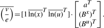
Given the data matrices

find parameters C≜[B^x B^u]^T solving the regression problem

(6)

where ε∈ℝ^q×m is measurement noise on W.

Notice that the parameter vector a no longer appears in the regression problem, but an estimate of it can be recovered from estimates of C=[B^x B^u]^T by way of Equation (4).

In the remainder of the article, we make the assumption that each column ε_·i of ε follows a Gaussian distribution, indicated by ε_·i~𝒩(0,Σ_εi), where Σ_εi is diagonal, i.e. the measurement errors in different experiments are mutually uncorrelated. We further assume that ε_.i is independent of ε_.j for i≠j. Then, Problem 1 can be subdivided into m independent subproblems, one for each reaction i:

(7)

where w_·i and c_·i are the ith columns of W and C, respectively.

The values of the parameter matrices B^x and B^u admit an interesting biological interpretation. Notice that one can immediately find values x₀∈ℝⁿ₊, u₀∈ℝ^p₊, e₀∈ℝ^m₊ and v₀∈ℝ^m such that , , and . As a consequence, Equation (5) can be rearranged into the common relative formulation of linlog models,

(8)

where 1_m is an m×1 vector of ones, (v₀,x₀,u₀,e₀) is a so-called reference state (Heijnen, 2005) and B^x₀, B^u₀ are matrices of elasticity constants, where

(9)

The elasticities, introduced in the context of Metabolic Control Analysis (MCA) (Heinrich and Schuster, 1996), describe the normalized local response of the reaction rates to changes in metabolite concentrations. The interest is that they can thus be immediately computed from the values of B^x and B^u found by the solution of Problem 1, and the equality .

Although straightforward in theory, solving the regression problem (6) encounters two complications in practice.

1. Since the measurements are carried out at (quasi-)steady state, we have N·v(x,u,e)=0. This introduces dependencies among the data and thus reduces the information content of the data matrix Y, in the sense that Y becomes rank deficient. Like in earlier work (Nikerel et al., 2009), we use standard approaches to solve this problem. We notably rely on principal component analysis (PCA) (Jolliffe, 1986; Nikerel et al., 2009) applied to the data matrix Y to reduce the model order, i.e. the number of independent parameters, and ensure well-posedness of the regression problem (see Supplementary Section S1 for technical details). In summary, we use singular value decomposition (SVD), a technique decomposing the data matrix into dominant and marginal components according to a variance criterion. For the purpose of linear regression, this corresponds to decomposing the parameter vector into a reduced number of components that can be determined with certainty based on the data, while the remaining components are poorly determined, i.e. they are ‘nonidentifiable’, and are discarded with negligible effect on the fit. We note in passing that the columns of W and Y are zero-mean, an important requirement for the correctness of the outlined analysis.

2. The high-throughput datasets contain a substantial amount of missing values, due to experimental limitations or instrument failures. If, for any given reaction, we only used the datapoints in which all relevant metabolite concentrations, enzyme concentrations and metabolic fluxes playing a role in that reaction are available, then a large amount of data would have to be thrown away. In practice, we would run the risk that the parameters cannot be reliably identified. The development of a method that is capable of maximally exploiting the information contained in incomplete datasets for solving Problem 1 is the main subject of the article and will be fully developed in the later sections.

3 LIKELIHOOD-BASED IDENTIFICATION OF LINLOG MODELS FROM MISSING DATA

For every reaction i, we are concerned with the problem of estimating the unknown parameters c_·i of the model given in (7) in the case where some entries of Y are unknown. We address the estimation problem by a maximum-likelihood approach, which is known to yield optimal (unbiased and minimum variance) estimates for our problem setting in the case where Y is fully known. As the problem is identical for all reactions i, in the remainder of the section we will drop for simplicity index ·i from the notation.

Let ℐ be the set of indices (row, column) corresponding to the known entries of Y, i.e. (j,k)∈ℐ if and only if Y_j,k is available. It is convenient to introduce the decomposition , where

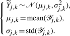
Matrix is fully determined: Once measurements of are collected, we treat as fixed parameters of the regression problem. Matrix collects the unknown entries of Y. We model these missing data as unobserved independent random variables, whose prior distributions encode our generic knowledge about them. Assuming that the a priori distributions are not known (worst case), we define a Gaussian prior for each quantity that is missing in an experiment based on the measurements of the same quantity available from other experiments. For every (j,k)∉ℐ and 𝒴_j,k={Y_j′,k: (j′,k)∈ℐ} (assumed nonempty), we let

(10)

We can now formulate the estimation problem.

Problem 2. —

Given measurements W=w and , compute the estimate ĉ=arg max_c log ℒ(c), with , where, for any c, is the probability density function of W given corresponding to model (7)–(10).

Note that ℒ(c) is a likelihood function for a linear model with missing data, in the sense that it is defined with respect to available data only. One can express ℒ(c) by marginalization,

(11)

where is the standard likelihood function for model (7) given and , with varying over all possible values of , and is determined by the prior (10). The explicit solution to the integral is reported in Supplementary Section S2. A direct approach to solving Problem 2 is to maximize (11) by numerical optimization. However, the function is not convex in c, whence its direct optimization is prone to end up in local minima and the use of global optimization strategies is required.

Alternatively, we propose to tackle Problem 2 by an Expectation-Maximization (EM) algorithm (Dempster et al., 1977). EM provides a general methodology for the optimization of a likelihood function with missing information. It is based on an iterative two-step procedure that, for the problem at hand, we implement as follows. Let us define the random variable , so that model (7) becomes . Note that 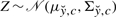, where for any given c, mean and variance can be derived from (10). Let ĉ⁰ be an initial guess of c. At every iteration ℓ=1,2,3,…, compute an updated estimate ĉ^ℓ from the estimate ĉ^ℓ−1 at the previous iteration by performing the following EM steps:

Expectation: compute

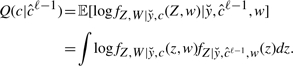(12)

Maximization: solve

(13)

In (12), is the joint probability density function of Z and W given and c, while , w is the probability density function of Z given , W=w and ĉ^ℓ−1. These quantities are easily expressed in terms of model (6) and the priors defined in (10) (see Supplementary Section B).

It can be proven that, at every iteration ℓ, the EM algorithm increases the value of ℒ(ĉ^ℓ, and eventually converges to a maximum of ℒ (Little and Rubin, 2002). While this is not necessarily a global maximum, EM has proven effective in many applications (Graham, 2009; Horton and Kleinman, 2007). A key property is that convergence to a maximum is achieved even if (13) is not solved exactly: It suffices that ĉ^ℓ is such that Q(ĉ^ℓ|ĉ^ℓ−1)≥Q(ĉ^ℓ−1|ĉ^ℓ−1), which is easily achieved even by a local optimization algorithm. In practice, we can use the explicit expression of ℒ in Problem 2 for stopping the iterations, e.g. when the relative improvement on ℒ falls below a specified threshold τ>0:

To complete the implementation of the algorithm, one must express Q(c|ĉ^ℓ−1) in a form convenient for maximization. As explained in Supplementary Section S2, one can express (12) as an explicit function of c for any given ĉ^ℓ−1. In compact form:

(14)

where f_c stands for a Gaussian distribution with variance and mean 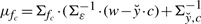, κ_fc is a function depending on c via μ_fc and Σ_fc, and the proportionality factor that we dropped (indicated by the presence of ∝ in place of =) depends on ĉ^ℓ−1 but not on c. Finally, KL(·||·) and H(·) are the Kullback–Leibler distance between distributions and the entropy of a distribution, respectively, for which, in the Gaussian case at hand, explicit formulas are available (Cover and Thomas, 2006; Stoorvogel and van Schuppen, 1996). A slight technical complicacy is needed in case is singular (see Supplementary Section S2 for all the mathematical details).

The availability of the closed-form expression (14) allows us to implement EM efficiently, i.e. with an explicit maximization problem that is solved numerically at all iterations. Once the parameter estimates are obtained, several methods from the literature can be used to assess the accuracy of the results by inferring confidence intervals. Examples are randomized methods such as bootstrapping (Manly, 1997) and the profile likelihood method by (Raue et al., 2009). This method derives confidence intervals using a threshold on a function called the profile likelihood. In our application, this is obtained separately for each parameter c_j by re-maximization of (11) with respect to all parameters c_k≠j, for all values c_j in a neighborhood of ĉ_j.

4 VALIDATION ON SYNTHETIC DATA

Before applying the EM algorithm to actual biological identification problems, we test the performance of the method on simulated data. For this purpose, a synthetic model has been developed, a simplified variant of the linlog model of E.coli central metabolism studied in Section 5 below. The model, in the form (2), contains 17 variables, representing internal and external metabolites involved in 25 reactions, and 78 parameters (see Supplementary Section S3 for the model equations). We generate data matrices Y from this model by means of simulation, for different percentages of missing data and experimental noise. Using the model structure and the simulated data, we solve Problem 1 for each reaction independently, as described in Section 3.

In order to assess the added value of our specific implementation of likelihood optimization, we first compare the performance of the EM algorithm of Section 3 with the direct maximization of the loglikelihood (11) implemented with a general-purpose Matlab optimization routine. This method will be referred to as MaxLL in the sequel.

Second, we compare the likelihood-based identification approaches with standard methods, notably linear regression (referred to as Rg) and the commonly-used multiple imputation (MI) method (Rubin, 1976; 1996). Regression is performed based on full datasets only, i.e. it does not consider an experimentally-determined datapoint (v^(k),x^(k),u^(k),e^(k)) when at least one of the measurements is missing. MI is based on imputation of missing data by random draws of the missing values, i.e. non-zero elements of , from the a priori distribution defined in (10). Both methods thus exploit only part of the information contained in an incomplete dataset and provide a lower limit for quantifying the performance of the methods proposed in Section 3.

Third, we compare the results of EM with the least-squares identification of the model on complete datasets (a method referred to as RgF, where F stands for Full datasets). Though inapplicable to real data with missing measurements, the method is statistically optimal. Hence, it provides us an upper performance bound that can be used to assess the role of missing data in performance degradation, separately from the role of noise.

Most of the high-throughput datasets available in the literature have been obtained when metabolism is at (quasi-)steady-state (Section 2). In order to mimic available experimental data as closely as possible, simulated data obtained from the synthetic model should therefore be steady-state data. We generated steady states of (1)–(2), and recorded the corresponding metabolite concentrations and metabolic flux values for 30 different conditions, each consisting of a random change in the enzyme concentration with respect to a reference value.

We compared performance of the five methods described above (EM, MaxLL, MI, Rg, RgF) on datasets with different amounts of missing data (40% and 75%) for the metabolite concentrations and noise levels (10% and 20%) for w. The only difference with the dataset used for the reference method RgF is that the latter has no missing data. A noise level of 10% means that the distribution used to generate the noise has a standard deviation equal to 10% of the values in w. The percentages of missing data in the simulation study are comparable to those observed in practice [Section 5 and (Ishii et al., 2007)]. For every different combination of missing data percentage and noise level, a dataset was generated by homogeneously distributing missing data among columns of Y, the indices for each column being chosen at random. For every simulated scenario, randomly generated noise was added to w in the dataset.

For all of the above scenarios, identification of each reaction was addressed separately, in accordance with the discussion of Section 2. For every reaction, we first tested the identifiability of the synthetic linlog model by PCA of the full data matrix Y. In our simulation, 9 reactions out of the 25 composing the model were detected as having nonidentifiable parameters. For those reactions, identification of a reduced-order model

(15)

was performed in place of the identification of the original model. Y*∈ℝ^q×r, with r≤n+p, is a reduced-order data matrix obtained by linear transformation of Y, and c*∈ℝ^r is a parameter vector, smaller than c, that is ‘identifiable’, in the sense that it is well determined by the data (see Supplementary Section S3).

We implemented the different parameter estimation algorithms in Matlab, using the lscov function for the regression-based methods and fminsearch for global optimization in MaxLL and the maximization step in EM. Both EM and MaxLL require an initial guess of the parameters to be specified. We proposed 10 different initial parameter vectors, including the estimation obtained with the baseline method Rg where available. In order to draw statistics for the estimation performance, each of the five algorithms was applied on 100 Monte-Carlo repetitions of the identification problem. The complete performance test over all methods, conditions and 100 repetitions took about 7 h 40 min in Matlab 7.4.0 on a Linux PC workstation (1862 MHZ, 2 GB RAM).

The most informative results from all identification methods are summarized by boxplots of the ratio of the estimated parameter values c over the reference parameter values c_ref used to simulate the data. The closer the ratio to 1, the better the estimates. Ensemble statistics are drawn for all parameters corresponding to the same reaction. Figure 1 is dedicated to the scenario with 40% missing data and 10% noise, whereas Figure 2 reports on 75% missing data and 20% noise. Complete results for all reactions under all conditions can be found in Supplementary Section S3.

Fig. 1.

Statistics of estimated parameter values for datasets with 40% of missing data and 10% noise. The results are shown as boxplots of the ratio of the estimated parameter values c and reference parameter values c_ref. Statistics have been computed for each of the 5 methods from 100 datasets. For each method, the red line displays the median and the lower and upper blue lines represent the lower and upper quartile values, respectively. Whiskers extend from each end of the box to the most extreme values within 1.5 times the interquartile range from the ends of the box and outliers are shown with red crosses. The tested algorithms are Expectation Maximization (EM), direct optimization of loglikelihood (MaxLL), multiple imputation (MI), regression on incomplete datasets (Rg) and regression on complete datasets (RgF). (A–D) Boxplots for reactions 3, 4, 11 and 18 of the network, respectively.

Fig. 2.

Statistics of estimated parameter values for datasets with 75% of missing data and 20% noise. The graphical notations are the same as for Figure 1. (A–F) Boxplots for reactions 3, 13, 17, 22, 19 and 25 of the network, respectively.

Since the individual reactions of the model involve only a small subset of metabolites, each of the m identification subproblems consists of the estimation of a limited number of parameters, mostly 2 or 3. For the case with 40% missing data, Rg can therefore be performed in all runs for every reaction of the model. On the contrary, with 75% missing data, regression cannot be applied to 6 reactions which is apparent from the absence of the Rg statistics for 2 reactions in Figure 2.

In comparison with the other methods, multiple imputation (MI) gives the worst results (largest bias) in 3 out of the 4 reactions shown in Figure 1, and in 5 out of 6 reactions in Figure 2. In reactions 11 of Figure 1 and 22 of Figure 2, the relatively small biases are accompanied by an estimation uncertainty wider than for EM and MaxLL. This could be explained by a restricted use of information contained in the distribution of missing data. Indeed, MI only considers random draws from the distribution while EM and MaxLL are based on all possible values taken by missing data through integration of the distribution.

Analysis of Figure 1 reveals that, for 40% missing data and 10% noise, the performance of EM and MaxLL is almost identical and similar to that of regression (Rg and RgF), with limited improvements on Rg, i.e. slightly smaller variability. In some cases, such as for reactions 11 and 18, their performance approaches the optimal, unattainable bound provided by RgF, i.e. they have similar bias and variability.

Performance improvements of likelihood-based methods over Rg become more significant when identification is performed on the dataset with higher percentage of missing data and larger noise. Figure 2A–D show results for reactions where Rg was applicable. Both EM and MaxLL substantially reduce estimation variability in reactions 3, 17 and 22. At the same time, due to the larger amount of missing data, performance loss with respect to RgF is more significant. Turned another way, this shows the accuracy that could be recovered were all datasets complete.

Figure 2E and F show the results when Rg fails to produce estimates and cannot be used to initialize EM and MaxLL optimization. Still, EM provides estimates of the right order of magnitude and, for the case of Figure 2E, of the right sign in at least 75% of the runs (box entirely above 0), while the median has the right sign and is reasonably close to 1. The estimation of the sign provided by MaxLL is less reliable (box crossing 0).

Overall, we conclude that the EM-based approach provides the most accurate estimates under all simulated conditions. We will therefore apply this method to the identification of the linlog model of an actual metabolic network from a published high-throughput dataset.

5 Application to central metabolism in E.coli

The network of central carbon metabolism in E.coli has been studied for a long time from different perspectives, which makes it an ideal model system for our purpose. A rather precise idea of the structure of the network exists, several kinetic models of the network dynamics are available [(Bettenbrock et al., 2005; Kotte et al., 2010) and references therein], and recently a high-throughput dataset containing the required information for solving Problem 1 has been published (Ishii et al., 2007). The network we consider here gathers enzymes, metabolites and reactions that make up the bulk of E.coli central carbon metabolism, including glycolysis, the pentose-phosphate pathway, the tricarboxylic acid cycle and anaplerotic reactions such as glyoxylate shunt and PEP-carboxylase (Fig. 3).

Fig. 3.

Scheme of E.coli central carbon metabolism. This map, showing metabolites (bold fonts) and genes (italic) is adapted from (Ishii et al., 2007). Abbreviations of metabolites are glucose (Glc), glucose 6-phosphate (G6P), fructose 6-phosphate (F6P), fructose 1-6-biphosphate (FBP), dihydroxyacetone phosphate (DHAP), glyceraldehyde 3-phosphate (G3P), 3-phosphoglycerate (3PG), phosphoenolpyruvate (PEP), pyruvate (Pyr), 6-phosphogluconate (6PG), 2-keto-3-deoxy-6-phospho-gluconate (2KDPG), ribulose 5-phosphate (Ru5P), ribose 5-phosphate (R5P), xylulose 5-phosphate (X5P), sedoheptulose 7-phosphate (S7P), erythrose 4-phosphate (E4P), oxaloacetate (OAA), citrate (Cit), isocitrate (IsoCit), 2-keto-glutarate (2KG), succinate-CoA (SuccoA), succinate (Suc), fumarate (Fum), malate (Mal), glyoxylate (Glyox), acetyl-CoA (AcoA), acetylphosphate (Acp) and acetate (Ace). Cofactors impacting the reactions are not shown. The gene names are separated by a comma in the case of isoenzymes, by a colon for enzyme complexes, and by a semicolon when the enzymes catalyze reactions that have been lumped together in the model.

The dataset used for identification of this network was obtained by experiments with 24 single-gene disruptants that were grown at a fixed dilution rate of 0.2 h⁻¹ in a glucose-limited chemostat, and with wild-type cells at 5 different dilution rates (Ishii et al., 2007). The authors collected data using multiple high-throughput techniques, in particular DNA microarray analysis and 2D differential gel electrophoresis (2D-DIGE) for genes and proteins, capillary electrophoresis time-of-flight mass spectrometry (CE-TOFMS) for metabolites, and metabolic flux analysis. They thus obtained a dataset consisting of metabolite concentrations, mRNA and protein concentrations for the enzymes, and metabolic fluxes under 29 different experimental conditions. A large number of different metabolites were measured in the experiments, with missing data in varying amounts, from 0 to 80% of the observations, 28% on average for the metabolites considered below.

From the reactions listed in (Ishii et al., 2007), we have constructed a linlog model of the form (2), with n=16 internal metabolites, p=7 external metabolites and measured cofactors, and m=31 reactions (see Supplementary Section S4). Each of the reactions is catalyzed by a single enzyme, which may actually stand for several enzymes in the case of isoenzymes, enzyme complexes or lumped reactions. Reactions have been simplified or lumped together when a shared metabolite has not been measured, which precludes estimation of the corresponding elements in the parameter matrices B^x and B^u. In comparison with an earlier linlog model of E.coli central carbon metabolism (Visser et al., 2004), we extended the scope to include the tricarboxylic acid cycle and the glyoxylate shunt, but due to the above-mentioned simplifications our model is more coarse-grained.

An identifiability analysis was performed by several rounds of missing data imputation using the a priori distribution defined in Equation (10) and PCA, which led in each case to the same result: 7 out of 31 reactions were detected as having nonidentifiable parameters. For those reactions, the model has been reduced as described in Equation (15) using a data matrix Y completed by the means μ_j,k of the a priori distributions. For every individual reaction, the reduced model has a parameter vector c* that is now entirely identifiable.

Apart from the distribution of the a priori missing data, given by Equation (10), application of EM requires information about the distribution of ε, the error on the ratios of fluxes and enzyme concentrations. The Ishii dataset provides several replica measurements for a reference experimental condition: wild-type cells grown in a glucose-limited chemostat with a dilution rate of 0.2 h⁻¹. These data were used for the computation of the variance of ε. In order to assess the accuracy of the estimated B^x and B^u, we computed for each parameter a 95% confidence interval, by means of the profile likelihood method outlined in Section 3. Running the EM method on the model and the data took about 220 s using the implementation of Section 4. The computation of the confidence intervals for all parameters required about 23 min.

Contrary to the simulation studies reported in Section 4, a reference or ‘real’ model for the evaluation of the results does not exist in this case. However, a priori biochemical knowledge on the signs of the elasticities is available, i.e. elasticities are positive for substrates and negative for products. This information can be compared with the estimated signs of the elasticities, and their confidence intervals, computed from the parameter matrices using the relations in Equation (9). The results are shown in Table 1. Similar unshown results are obtained by means of the MaxLL method.

Table 1.

Elasticity matrix [B₀^x B₀^u] estimated by EM from the data of (Ishii et al., 2007) for the linlog model of E.coli central carbon metabolism (the columns of the matrix have been permuted for readability)

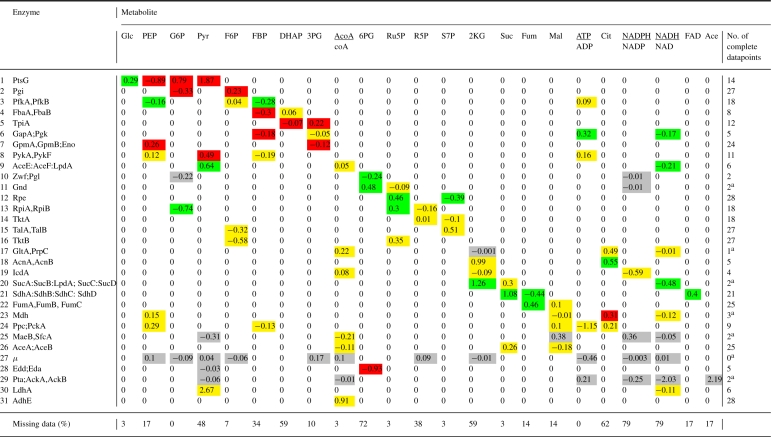Unidentifiable elasticities are shown in grey, uncertain elasticities (i.e. having a sign that is not significant with 95% confidence) in yellow, and correctly/incorrectly identified elasticities (i.e. having a sign that is significant with 95% confidence) in green/red. Abbreviations are as in Figure 3. Some of the cofactors are modeled as ratios of metabolite concentrations, e.g. ATP/ADP. Reaction 27, labeled μ, is a phenomenological reaction for biomass production. The last row indicates the percentage of missing data per metabolite and the right-most column displays the amount of complete datapoints available for each reaction. ^aRegression was not able to produce any result.

We observe that the EM method obtains estimates for all reactions, including the 7 cases where the insufficient amount of data made regression not applicable. However, 26 of the 100 non-zero elasticities of the model are not identifiable from this dataset. Moreover, out of the remaining 74 elasticity estimates, more than half of them have signs that are not statistically significant, in the sense that the 95% confidence interval straddles 0. This is most likely due to the fact that the magnitude of noise in metabolite concentrations is comparable to the magnitude of relevant information. For example, for PEP the standard deviation over all experimental conditions equals the standard deviation of the replicates in a single condition (0.06 mM versus 0.05 mM). This precludes the estimation of an unambiguous sign.

Of the elasticities with statistically significant signs, 20 out of 34 are correct, in the sense that they have the expected positive or negative sign. The remaining elasticities, distributed over 9 reactions, are incorrectly estimated. Let us now discuss what we believe are potential sources of these errors, giving information that could be used to single out erroneous estimates a priori.

We first note that for 3 of these 9 reactions (GapA;Pgk, Mdh and Edd;Eda, see Table 1), only very few complete datapoints are available (between 3 and 5) and regression mostly fails in these cases. In addition, all of these reactions involve at least one metabolite missing in >70% of the experimental conditions. The combination of very few complete datapoints and a high percentage of missing metabolite measurements obviously makes model identification extremely difficult and it is fair to say that here we reach the limit of the applicability of our method, or of any method for that matter, due to the lack of data.

Second, 4 reactions are known to operate close to equilibrium: Pgi, FbaA,FbaB, TpiA and GpmA,GpmB;Eno (Visser et al., 2004). Theoretically, these reactions are not identifiable, as their elasticities are not independent (Visser et al., 2004), but PCA did not detect this. Most likely, this is due to the above-mentioned noise in metabolite concentrations, which decreases their correlations. A cautious, preemptive strategy would be to reduce the model for any reaction known to be close to equilibrium and eliminate the corresponding dependent variables.

The errors in the signs of some elasticities in the remaining 2 reactions (PtsG and PykA,PykF) are less straightforward to explain. It is unlikely that they can be attributed to the EM method, given that regression is applicable here with a relatively large number of complete datapoints available (14 and 11, respectively) and gives the same results. Alternatively, they may be explained by a modeling error or a hidden variable, for instance an unknown cofactor, biasing the estimation results. It is also possible that the approximations of the linlog model are not suitable for these reactions, for instance because there are large variations in metabolite concentrations between conditions, driving the system far from the reference state.

In summary, EM gives reasonable results for a fairly complicated model on a challenging dataset. Even though some puzzling issues remain, we believe that these can be safely attributed to the inherent difficulty of the identification problem.

6 DISCUSSION

In this work, we have addressed the problem of estimating parameters of approximate models of metabolic networks from incomplete datasets. Even with the largest datasets available at present, such as those reported in (Ishii et al., 2007), the absence or corruption of a large number of measurements may reduce the effective number of datapoints to a handful of experimental conditions, thus making simple regression techniques ineffective or even inapplicable. Making full use of all the available data is therefore essential to render identification well-posed and improve the quality of the estimated models.

To this aim, we have proposed a maximum-likelihood method for the identification of linlog metabolic network models that compensates for the missing data by the use of statistical priors. We developed an algorithm that attains maximization of the likelihood based on Expectation Maximization, a well accepted paradigm for the numerical optimization of likehood functions in the presence of unobserved variables. A simpler implementation based on direct likelihood maximization via general-purpose numerical optimization algorithms was also considered and found slightly less powerful. The performance of EM was compared to that of an existing method of reference, namely multiple imputation, and to worst-case and best-case scenarios given by least-squares regression on the sole complete datapoints and on complete datasets, respectively. We showed that EM outperforms multiple imputation by a wide margin. In comparison with worst-case regression, it reduces the estimation variability and is able to produce reasonable estimation results even when regression on incomplete datasets is inapplicable. It also approaches the ideal performance of regression on complete datasets for low rates of missing data, regardless of noise.

Based on these findings, we applied EM to the identification of a linlog model for the central carbon metabolism in the bacterium E.coli from the experimental data presented by Ishii et al. (2007). Even with the large amount of incomplete datapoints, due to the difficulty of experimentally measuring metabolite concentrations, EM was able to estimate many of the model parameters (elasticities) in agreement with the current understanding of the system. This is even true for reactions where the reduced number of complete datapoints impairs the applicability of least squares regression. On the other hand, the challenging quality of the data sheds light on the performance limits of the method, which tends to fail when large measurement noise makes the estimation of small parameters statistically unreliable, when the same variable cannot be measured in most conditions, or when reactions operate near equilibrium.

Overall, results from the simulations and the application on real data showed that our EM approach is able to make the most of incomplete, noisy high-throughput datasets for the estimation of parameters in approximate kinetic models. In the future, we expect to improve performance by developing a number of technical points, including approximate analytical/dedicated numerical solutions for the EM maximization steps, the refinement of the identifiability analysis via SVD of incomplete data matrices (Brand, 2002), and a more detailed modeling of measurement noise. It is worth noting that, while the method has been developed for linlog models, it is more generally applicable to any other metabolic network model that can be put in a form linear in the parameters by straightforward manipulations, such as generalized mass action models that provide advantages when some metabolite concentrations approach 0 (Savageau, 1976; del Rosario et al., 2008). In addition, estimated parameters of approximate metabolic models, such as elasticities of linlog models, provide useful hints for the identification of more detailed nonlinear kinetic models.

From a broader perspective, the application of the EM method to a unique multi-omics dataset for E.coli carbon metabolism allowed us to isolate issues that are critical for the appropriate exploitation of the data for parameter estimation. These issues may need to be taken into account during the design of the experiments. One such issue is that a high percentage of missing data for some of the individual variables, even at a relatively low average percentage over the entire dataset, was found to be much detrimental to the identification results. This may influence sampling strategies, especially for metabolites that are difficult to measure. Another issue is the identifiability problems caused by steady-state measurements, which cannot always be resolved by genetic mutation or by varying physiological conditions. From this perspective time-resolved observations of the network dynamics, although much more demanding experimentally, carry great promise (Hardiman et al., 2007).

REFERENCES

- Ashyraliyev M., et al. Systems biology: Parameter estimation for biochemical models. FEBS J. 2009;276:886–902. doi: 10.1111/j.1742-4658.2008.06844.x. [DOI] [PubMed] [Google Scholar]
- Bettenbrock K., et al. A quantitative approach to catabolite repression in Escherichia coli. J. Biol. Chem. 2005;281:2578–2584. doi: 10.1074/jbc.M508090200. [DOI] [PubMed] [Google Scholar]
- Brand M. Incremental singular value decomposition of uncertain data with missing values. In: Heyden A., editor. Proceedings of the 7th European Conference Computer Vision (ECCV 2002) Vol. 2350. Berlin/Heidelberg: Springer; 2002. pp. 707–20. of Lecture Notes in Computer Science. [Google Scholar]
- Costa R., et al. Hybrid dynamic modeling of Escherichia coli central metabolic network combining Michaelis-Menten and approximate kinetic equations. Biosystems. 2010;100:150–158. doi: 10.1016/j.biosystems.2010.03.001. [DOI] [PubMed] [Google Scholar]
- Cover T., Thomas J. Elements of Information Theory. 2. New York: Wiley; 2006. [Google Scholar]
- Crampin E. Proceedings of the 14th IFAC Symposium System Identification (SYSID 2006) Newcastle, Australia: 2006. System identification challenges from systems biology; pp. 81–93. [Google Scholar]
- del Rosario R., et al. Challenges in lin-log modelling of glycolysis in Lactococcus lactis. IET Syst. Biol. 2008;2:136–149. doi: 10.1049/iet-syb:20070030. [DOI] [PubMed] [Google Scholar]
- Dempster A., et al. Maximum likelihood from incomplete data via the EM algorithm. J. Roy. Stat. Soc. Ser. B. 1977;39:1–38. [Google Scholar]
- Graham J. Missing data analysis: Making it work in the real world. Annu. Rev. Psychol. 2009;60:549–576. doi: 10.1146/annurev.psych.58.110405.085530. [DOI] [PubMed] [Google Scholar]
- Hadlich F., et al. Translating biochemical network models between different kinetic formats. Metab. Eng. 2009;11:87–100. doi: 10.1016/j.ymben.2008.10.002. [DOI] [PubMed] [Google Scholar]
- Hardiman T., et al. Topology of the global regulatory network of carbon limitation in Escherichia coli. J. Biotechnol. 2007;132:359–374. doi: 10.1016/j.jbiotec.2007.08.029. [DOI] [PubMed] [Google Scholar]
- Hatzimanikatis V., Bailey J. Effects of spatiotemporal variations on metabolic control: Approximate analysis using (log)linear kinetic models. Biotechnol. Bioeng. 1997;54:91–104. doi: 10.1002/(SICI)1097-0290(19970420)54:2<91::AID-BIT1>3.0.CO;2-Q. [DOI] [PubMed] [Google Scholar]
- Heijnen J. Approximative kinetic formats used in metabolic network modeling. Biotechnol. Bioeng. 2005;91:534–545. doi: 10.1002/bit.20558. [DOI] [PubMed] [Google Scholar]
- Heinrich R., Schuster S. The Regulation of Cellular Systems. New York: Chapman & Hall; 1996. [Google Scholar]
- Horton N., Kleinman K. Much ado about nothing: a comparison of missing data methods and software to fit incomplete data regression models. Am. Stat. 2007;61:79–90. doi: 10.1198/000313007X172556. [DOI] [PMC free article] [PubMed] [Google Scholar]
- Ishii N., et al. Multiple high-throughput analyses monitor the response of E. coli to perturbations. Science. 2007;316:593–597. doi: 10.1126/science.1132067. [DOI] [PubMed] [Google Scholar]
- Jolliffe I. Principal Component Analysis. New York: Springer; 1986. [Google Scholar]
- Kotte O., et al. Bacterial adaptation through distributed sensing of metabolic fluxes. Mol. Syst. Biol. 2010;6:355. doi: 10.1038/msb.2010.10. [DOI] [PMC free article] [PubMed] [Google Scholar]
- Liebermeister W., Klipp E. Bringing metabolic networks to life: Convenience rate law and thermodynamic constraints. Theor. Biol. Med. Model. 2006;3:41. doi: 10.1186/1742-4682-3-41. [DOI] [PMC free article] [PubMed] [Google Scholar]
- Little R., Rubin D. Statistical Analysis with Missing Data. Hoboken, New Jersey: Wiley; 2002. [Google Scholar]
- Manly B. Randomization, Bootstrap and Monte-Carlo Methods in Biology. Chapman and Hall; 1997. [Google Scholar]
- Marucci L., et al. Derivation, identification and validation of a computational model of a novel synthetic regulatory network in yeast. J. Math. Biol. 2011;62:685–706. doi: 10.1007/s00285-010-0350-z. [DOI] [PubMed] [Google Scholar]
- Nikerel I., et al. A method for estimation of elasticities in metabolic networks using steady state and dynamic metabolomics data and linlog kinetics. BMC Bioinformatics. 2006;7:540. doi: 10.1186/1471-2105-7-540. [DOI] [PMC free article] [PubMed] [Google Scholar]
- Nikerel I., et al. Model reduction and a priori kinetic parameter identifiability analysis using metabolome time series for metabolic reaction networks with linlog kinetics. Metab. Eng. 2009;11:20–30. doi: 10.1016/j.ymben.2008.07.004. [DOI] [PubMed] [Google Scholar]
- Oba S., et al. A Bayesian missing value estimation method for gene expression profile data. Bioinformatics. 2003;19:2088–2096. doi: 10.1093/bioinformatics/btg287. [DOI] [PubMed] [Google Scholar]
- Raue A., et al. Structural and practical identifiability analysis of partially observed dynamical models by exploiting the profile likelihood. Bioinformatics. 2009;25:1923–1929. doi: 10.1093/bioinformatics/btp358. [DOI] [PubMed] [Google Scholar]
- Rubin D. Inference and missing data. Biometrika. 1976;63:581–590. [Google Scholar]
- Rubin D. Multiple imputation after 18+ years. J. Am. Stat. A. 1996;81:473–489. [Google Scholar]
- Savageau M. Biochemical Systems Analysis: A Study of Function and Design in Molecular Biology. MA: Addison-Wesley, Reading; 1976. [Google Scholar]
- Scholz M., et al. Non-linear PCA: A missing data approach. Bioinformatics. 2005;21:3887–3895. doi: 10.1093/bioinformatics/bti634. [DOI] [PubMed] [Google Scholar]
- Smallbone K., et al. Towards a genome-scale kinetic model of cellular metabolism. BMC Syst. Biol. 2010;4:6. doi: 10.1186/1752-0509-4-6. [DOI] [PMC free article] [PubMed] [Google Scholar]
- Stoorvogel A., van Schuppen J. System identification with information theoretic criteria. In: Bittanti S., Picci G., editors. Identification, Adaptation, Learning. Vol. 153. Springer; 1996. pp. 289–338. of NATO ASI. [Google Scholar]
- Visser D., Heijnen J. Dynamic simulation and metabolic re-design of a branched pathway using linlog kinetics. Metab. Eng. 2003;5:164–176. doi: 10.1016/s1096-7176(03)00025-9. [DOI] [PubMed] [Google Scholar]
- Visser D., et al. Optimal re-design of primary metabolism in Escherichia coli using linlog kinetics. Metab. Eng. 2004;6:378–90. doi: 10.1016/j.ymben.2004.07.001. [DOI] [PubMed] [Google Scholar]
Associated Data
This section collects any data citations, data availability statements, or supplementary materials included in this article.