Correlating anomalous diffusion with lipid bilayer membrane structure using single molecule tracking and atomic force microscopy

Abstract

Anomalous diffusion has been observed abundantly in the plasma membrane of biological cells, but the underlying mechanisms are still unclear. In general, it has not been possible to directly image the obstacles to diffusion in membranes, which are thought to be skeleton bound proteins, protein aggregates, and lipid domains, so the dynamics of diffusing particles is used to deduce the obstacle characteristics. We present a supported lipid bilayer system in which we characterized the anomalous diffusion of lipid molecules using single molecule tracking, while at the same time imaging the obstacles to diffusion with atomic force microscopy. To explain our experimental results, we performed lattice Monte Carlo simulations of tracer diffusion in the presence of the experimentally determined obstacle configurations. We correlate the observed anomalous diffusion with obstacle area fraction, fractal dimension, and correlation length. To accurately measure an anomalous diffusion exponent, we derived an expression to account for the time-averaging inherent to all single molecule tracking experiments. We show that the length of the single molecule trajectories is critical to the determination of the anomalous diffusion exponent. We further discuss our results in the context of confinement models and the generating stochastic process.

INTRODUCTION

Transport in the plasma membrane of biological cells is essential to many protein mediated signaling events and so there is great interest in understanding the biophysical mechanisms controlling diffusion. Over the past two decades, single particle and single molecule tracking (SMT) has arisen as a powerful method to study the transport of membrane constituents.^{1, 2, 3} It reveals dynamic subpopulations and opens the possibility of studying the full statistical distributions of the transport process. Anomalous subdiffusion has been found to be common in the plasma membrane^{4, 5, 6} with important implications for protein complex formation⁷ and it implies that the plasma membrane is a complex and crowded environment.

Several mechanisms have been suggested as the source of the observed anomalous subdiffusion: obstruction by the membrane skeleton and its bound proteins,⁶ inclusion or exclusion from lipid domains,⁸ binding to immobile traps,^{9, 10} or a combination of the above.^{11, 12} Single particle tracking experiments to date could not directly image the obstacles to diffusion but only deduce their physical properties from the diffusion data.

The primary purpose of this work is to correlate single molecule tracking data with the obstacle properties in a system where we can image the obstacles directly with high resolution. We performed single molecule tracking in a 2-component phase separated lipid bilayer on a solid support. The two bilayer components were 1,2-distearoly-sn-glycero-3-phosphocholine (DSPC) and 1,2-dioleoyl-sn-glycero-3-phosphocholine (DOPC). Although supported lipid bilayers lack some features of a real cell membrane, their utility as an experimental platform has increased our understanding of cell membrane organization and dynamics.^{13, 14, 15, 16} Most importantly to our study, the supported bilayer allows imaging the submicron, gel phase domain obstacles with nanometer resolution using atomic force microscopy (AFM). We do not suggest that the obstacles in cell membranes are gel phase domains; in fact they are proteins, protein aggregates, and regions of ordered lipids. The lipid domains in our system function simply as area excluding obstacles, whose size and density can be easily controlled and imaged. They are analogous to the polymers and nanoparticles used to model the obstructed diffusion of the cell interior.^{17, 18} Parallel to the experiments, we used the AFM images as input into lattice Monte Carlo simulations to gain further insight into the results and statistics of the experiments. Our complementary results on the structure and dynamics of an obstructed membrane system, provide guidelines by which diffusion data can be used to determine the source of anomalous subdiffusion in cell membranes where the obstacles cannot be directly imaged.

Anomalous diffusion

Normal Brownian diffusion in two dimensions can be characterized by a single parameter, the diffusion coefficient D, which is the proportionality constant between a particle's mean-square displacement(MSD) 〈r²〉 and time lag t,

$$⟨r^2⟩=4Dt.$$ (1)

If some mechanism leads to a different power law dependence of 〈r²〉 on t, the diffusion is termed anomalous and it is characterized by two parameters,^{19, 20} the transport coefficient Γ and the anomalous diffusion exponent α,

$$⟨r^2⟩=4\Gamma t^{\alpha }.$$ (2)

The factor of 4 in Eq. 2 is unnecessary, but is chosen that in the case α = 1, Γ = D. If the mechanism hinders diffusion and α < 1, we call it anomalous subdiffusion. Sometimes, the fractal dimension of the random walk, d_w, is used in place of the anomalous diffusion exponent, where α = 2∕d_w. Diffusion may be anomalous over all times, such as diffusion on an infinite fractal²¹ or in the presence of an infinite hierarchy of binding sites,¹⁰ or it may only be transiently anomalous becoming normal at sufficiently long times,

$$⟨r^2⟩=\left\{\begin{array}{cc}\hfill 4\Gamma t^{\alpha }& \hfill t\ll t_{CR}\\ \hfill 4Dt& \hfill t\gg t_{CR}\end{array}\right..$$ (3)

The crossover time t_CR depends of the nature of the obstructions and D of the system.

If anomalous subdiffusion stems from obstacles, percolation theory connects obstacle characteristics and subdiffusive behavior^{22, 23} where the obstacles are characterized by an area fraction C, a percolation threshold C_p, and a correlation length ξ. C_p is the obstacle area fraction at which the obstacles connect into a network that spans the entire surface. The correlation length ξ is approximately the length scale of the obstacles;²³ on larger scales the surface is homogenous. For C<C_p, there are long range paths available to diffusing molecules. As the obstacle area fraction increases toward C_p, ξ, and t_CR increase, and α and D decrease. At the percolation threshold, C=C_p, all long range paths have been closed off by obstacles, D → 0, t_CR→∞, ξ → ∞ and α = const. The value of α at the percolation threshold depends on the fractal nature of the obstacles,²¹ but is close to 0.7.

MATERIALS AND METHODS

Materials and Methods are provided in the supplementary material.²⁴

RESULTS

Obstacle characterization

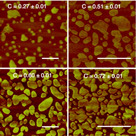
The primary benefit of performing this study on mica supported lipid bilayers is that the structure of the obstacles can be studied with suboptical resolution using AFM.^{25, 26} We take advantage of the fact that in a phase separated lipid bilayer, the DSPC rich, gel phase domains protrude ∼1.8 nm higher than the surrounding DOPC rich, fluid phase, providing the necessary height contrast for AFM to characterize the gel domain obstacles. Although we have not quantified the resolution in our AFM images, typical values are 0.1 nm in the vertical direction and 1.0 − 3.0 nm in the image plane.²⁷ Figure 1 shows representative images for different domain area fractions.

Figure 1.

Representative AFM images for the four highest domain area fractions studied. Scale bars are 1 μm. Slight differences in contrast are due to varying levels of instrument noise and background. Additional images are shown in Fig. 6 of the supplementary material (Ref. ²⁴).

The first characterization is the domain area fraction C, which is calculated by counting the number of pixels in an image above a selected height threshold. Figure 1 in the supplementary material is an AFM line scan illustrating the thresholding procedure.²⁴ For each composition, between five and eight images were recorded from different areas of the sample and the average domain area fraction (C) and standard error were calculated.

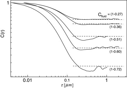
A more detailed characterization, which depends on the size and shape of the obstacles is the pair correlation function C(r), which is the probability of finding two fluid phase patches a distance r apart.²⁸ At distances less than the correlation length ξ, C(r) decreases with a power law dependence on the fractal dimension D_f of the fluid phase regions, in the same way that the density of a fractal object scales with length,²³ ρ(L)∼L^D_f−2. For r ≫ ξ, C(r) equals the average fluid phase area fraction C_fluid,

$$C\left(r\right)=\left\{\begin{array}{cc}\hfill 1& \hfill r=0\\ \hfill r^{-(2-D_f)}& \hfill r\ll \xi \\ \hfill C_{\text{fluid}}& \hfill r\gg \xi \end{array}\right..$$ (4)

Note that C_fluid=1−C, where C is the obstacle area fraction based on simple thresholding of the AFM images. D_f and ξ are both determined by the size and shape of the fluid regions and both influence the diffusive behavior of molecules in the fluid. This is only one possible definition of D_f. We use it because it has been used to effectively characterize the type of two dimensional objects we see in phase-separated lipid bilayers.²⁹ For a normal, two-dimensional object, D_f = 2 and for a line D_f = 1. Fractal objects have a D_f between these limits, typically in the range of 1.4 − 1.7.

C(r) was calculated using the fast Fourier transform.²⁴ Figure 2 shows for each composition a decrease in C(r) and then a plateau near the fluid area fraction as expected from Eq. 4. However, another plateau at small length scales appears because at distances smaller than the obstacle-obstacle separation, the fluid is unobstructed. This has also been observed for multicenter diffusion limited aggregates.²⁹ At low fluid area fraction, a depletion zone, caused by the area excluded by large gel domains, appears before C(r) reaches the average fluid area fraction.

Figure 2.

Pair correlation curves for each obstacle area fraction. All curves are an average from 5 to 8 images. C(r) is calculated up to a maximum of one half the image size. For some compositions this was 4 μm and for the others, adequate images were obtained only for 2 μm scans. Horizontal dashed lines show the average fluid phase area fraction, C_fluid=1−C, and are based on the measurements of obstacle area fraction.

Equation 4 allows the fractal dimension of the fluid region to be estimated by the slope of log [C(r)] at the inflection point. We find that as the fluid phase area fraction decreases (obstacle area fraction increases), D_f decreases (Table 1). This means that the fluid regions are becoming more elongated and tortuous. The correlation length ξ was estimated to be the point where C(r)=C_fluid. ξ increases with increasing obstacle area fraction as would be expected for an object approaching a percolation threshold.

Table 1.

Fluid phase area fraction C_fluid, fractal dimension D_f, and correlation length ξ. C_fluid is reported in terms of (1-C) to allow easier comparison with the AFM and MSD data which are reported in terms of C.

Cfluid	Df	ξ [μm]
(1-0.27)	1.81	0.15
(1-0.36)	1.75	0.31
(1-0.51)	1.56	0.66
(1-0.60)	1.41	0.62
(1-0.72)	1.35	0.62

Mean-square displacement

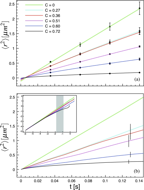
Using the raw position versus time data recorded in single molecule tracking and diffusion can be quantified in a variety of ways. Probability distributions of displacements can reveal dynamic subpopulations or anomalous diffusion and have been used in a number of studies.^{30, 31, 32, 33} We use the MSD for two reasons. First, with direct AFM images of the membrane obstacles, there is no reason to assume that there are two distinct dynamic populations. Second, there is no general form for the probability density in the case of a percolation cluster.²¹ Figure 3a shows the ensemble averaged mean-square displacement as a function of time lag for each obstacle density.

Figure 3.

Ensemble averaged mean-square displacement. (a) The symbols are experimental data and the solid lines are least square fits to Eq. 5. (b) Simulated data, presented on the same timescale as the experimental data. The error bars are the standard deviation between the MSD calculated on different AFM images. The inset is the full log-log representation of the simulated MSD data and the shaded region shows the time range over which the data were fitted with Eq. 2.

Sensitivity of fitting

A simple least square fit of the MSD to Eq. 2, implies an intercept 〈r²(t = 0)〉 = 0, but experimental uncertainty and error introduces a non-zero intercept. Martin et al. showed that the non-zero intercept can complicate the analysis of log-log MSD data, where a non-zero intercept was manifest as apparent subdiffusion.³⁴ Therefore we used a linear analysis of the MSD, but we found that the value of the anomalous diffusion exponent was very sensitive to the y-intercept. Including the intercept as a fitting parameter, in addition to adding a third fitting parameter, could result in a value of α that differs from the simple case by 20%. Therefore we needed a modified version of Eq. 2 to quantitatively account for the intercept.

It has been shown that two additional terms should be added to account for the non-zero intercept in the MSD,^{35, 36} which leads to the following form for the MSD:

$$⟨r^2⟩=4\Gamma t^{\alpha }+4{\left(\Delta x\right)}^2-{\Delta }_{\text{off}},$$ (5)

where Γ and α are the free parameters.

The term 4(Δx)², accounts for the localization precision of the experiments; in all cases we used 4(Δx)² = 0.0038μm² (see supplementary material²⁴). Δ_off is an offset introduced by the time averaging during each exposure. Goulian and Simon showed that for normal diffusion Δ_off=4Dt_ill∕3, where t_ill is the exposure time of each image.³⁵ We do not assume normal diffusion, so we need a more general expression for Δ_off where α is allowed to vary. We followed the same procedure but introduced the anomalous diffusion exponent α and the resulting analysis is presented in the supplementary material.²⁴ We find that the offset due to time averaging is Δ_off=8Γ(t_ill)^αδ(α), where δ(α) is approximated by the polynomial δ(α) ≃ 0.2573α² − 0.5688α + 0.4859. We fit Eq. 5 to the experimental MSD up to the fourth data point (n = 4). The resulting fit parameters Γ and α are presented in Table 2. We used standard methods to calculate the error in the MSDs and estimate the error in the fit parameters (see supplementary material²⁴).

Table 2.

Diffusion parameters obtained from least square fits of Eq. 2 and Eq. 5 to the simulated and experimental MSDs, respectively.

	Γ [μm2∕sα]		α
C	Expt.	Simulation	Expt.	Simulation
0	4.15 ± 0.27	4.22	0.97 ± 0.03	0.99
0.27	2.33 ± 0.06	2.57 ± 0.14	0.87 ± 0.01	1.00 ± 0.02
0.36	2.19 ± 0.02	2.26 ± 0.15	0.85 ± 0.003	0.96 ± 0.03
0.51	1.55 ± 0.003	1.92 ± 0.08	0.86 ± 0.001	1.00 ± 0.02
0.60	0.78 ± 0.01	0.72 ± 0.02	0.77 ± 0.004	0.84 ± 0.01
0.72	0.16 ± 0.0001	0.23 ± 0.04	0.56 ± 0.0003	0.59 ± 0.06

Figure 3b shows MSD curves from the simulated trajectories. Except for the unobstructed diffusion case which was scaled to match, the similarity between the experimental and Monte Carlo MSD curves is non-trivial. The inset of Fig. 3b shows that at very short times, diffusion is normal for all obstacle area fractions. Only at intermediate times the curves diverge and become anomalous. The length scale at which the MSD becomes anomalous corresponds to the transition in C(r) (Fig. 2) from a plateau at small r to a fractal region at intermediate r. For most AFM images, this occurs at r ∼ 0.02 μm or at a point on the MSDs of ⟨r²⟩∼4×10⁻⁴μm².

The diffusive behavior depends on the timescale, so to compare simulated diffusion parameters with experiment, the simulated MSDs must be fit over the same timescale as the experimental MSDs. The shaded band in the inset of Fig. 3b shows the time range over which the simulated MSDs were fit with Eq. 2. We use Eq. 2 for the simulated data, instead of Eq. 5, because there are none of the uncertainties that made Eq. 5 necessary for the experimental data. The measured values are presented in Table 2.

Anomalous diffusion exponent

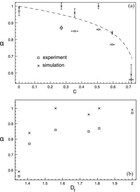
The degree of anomaly of a subdiffusive process is characterized by the anomalous diffusion exponent α, defined in Eq. 2. The primary aim of this work was to correlate anomalous diffusion with lipid bilayer structure, so we start by comparing α to obstacle area fraction in Fig. 4a (the relationship between Γ and the obstacle area fraction is presented in the supplementary material²⁴). In a pure fluid DOPC bilayer (C=0), α ∼ 1, showing normal diffusion. With increasing gel domain area fraction, the diffusion becomes gradually subdiffusive until α decreases more sharply near C=0.7, suggesting a percolation threshold near C=0.7. The rapid decrease of α near the percolation threshold is characteristic of a critical point and has been observed in other simulations.³⁷ Figure 4 shows that the experimental values of α are systematically lower than those from simulations. We believe there are two reasons for this (see Sec. 4). Percolation theory²¹ predicts at the percolation threshold, α ∼ 0.7, but in both the simulations and experiments α ∼ 0.58 at the highest area fraction. The AFM images (Fig. 1) suggest that we are still below the percolation threshold, but they also reveal small and completely enclosed fluid regions. Although the highest obstacle area fraction may be below the percolation threshold, some fluorescent tracers may be completely confined and contributing to a lower value of α.

Figure 4.

(a) The anomalous diffusion exponent as a function of obstacle area fraction. The dashed line is 2∕d_w with d_w given in Saxton (Ref. ³⁷) . (b) The dependence of the anomalous diffusion exponent on the fractal dimension of the fluid phase.

Correlating dynamics with structure

With high resolution images of the lipid domain obstacles, we can correlate the anomalous diffusion behavior with more than just the obstacle area fraction. Figure 4b shows the dependence of α on the fractal dimension of the fluid phase. The so-called AO conjecture²³ relates the anomalous diffusion exponent to the fractal dimension at the percolation threshold as αD_f ≃ 4∕3. Near the percolation threshold, we find αD_f ≃ 0.75 in poor agreement with the AO value of 4∕3. This is not too surprising as we believe α may be especially low at the highest obstacle area fraction due to small and enclosed areas of fluid.

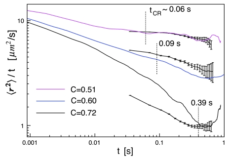
We can also test whether the crossover time and length scales from the MSDs predict the correlation lengths determined independently via AFM (Table 1). This is something that in general has not been possible experimentally. For the two lowest obstacle area fractions, ξ is below the length scale of the experiments and according to the simulations the normal long range behavior has already been reached at the experimental timescale. For the three highest area fractions, ξ from the AFM images is within the experimental length scale. Figure 5 shows the MSD data in a way that more clearly reveals transitions between dynamic regimes. A negative slope signifies α < 1 and where diffusion is normal, the plot is a constant. Figure 5 also shows t_CR based on the AFM obstacle analysis via ξ²=⟨r²⟩_tCR. For C=0.51, the crossover time is near the low end of the experimental timescale, but the transition can be seen in the simulated data at t ∼ 0.02 s. To match experimental timescales, the simulated MSDs were fit for 0.04<t<0.13 s, which explains why α ∼ 1 even for a relatively high obstacle area fraction of C=0.51. If the simulated MSD was fit for 0.0036<t<0.0144 s, α = 0.86. For C=0.60 the experimental and simulated MSDs show a transition near t ∼ 0.6 s, which does not agree with the t_CR∼0.09 s from the domain structure. If we only had the MSD data, as in typical experiments, we would predict an obstacle correlation length of 1.4 μm, which is 2-fold greater than measured by AFM. For C=0.72 where t_CR is well within the experimental timescale, the agreement is quite good between the experimental and simulated MSDs and the t_CR prediction.

Figure 5.

Log-log plot of 〈r²〉∕t versus t. The solid lines are simulated data. The solid lines with error bars are experimental data. The vertical dashed lines are t_CR from AFM analysis of the domain structure (Table 1). Experimental MSDs were truncated when errors became very large.

DISCUSSION

These results tell us several things about correlating anomalous diffusion with bilayer obstacle structure. The first is that the anomalous diffusion exponent follows the expected dependence on obstacle area fraction (Fig. 4a). We also find a similar relationship between α and the fractal dimension of the fluid phase (Fig. 4b). In cases where the obstacles to diffusion cannot be imaged, these results might be used to estimate the obstacle area fraction or fractal dimension. In terms of predicting the correlation length of the obstacles, the results were mixed. Only in the case of the highest obstacle area fraction, C=0.72, do we find good agreement between the correlation lengths determined via AFM and SMT. This result suggests that it may be difficult to measure the length scale of the bilayer obstacles given the diffusion data alone, even when the MSDs show a clear transition, such as in the case of C=0.60 (Fig. 5).

A persistent discrepancy between the experimental and simulated data was the systematically lower experimental values of α compared to the simulations. There are two factors that may have contributed to this difference. First is the choice of timescale over which the simulated MSDs were fit with Eq. 2. For C=0.27,0.36, and 0.51, the simulations give values of α close to one when fit over the experimental timescale, 0.04<t<0.13 s. If the simulated MSDs are fit over a lower time scale, 0.0036<t<0.0144 s, α is 5%14% lower. For these three compositions, the simulations predict a crossover time close to the lower limit of the experimental timescale, 0.035 s, which makes the value of α very sensitive to the fitting timescale. Considering this effect, the experimental α values are still systematically lower than the simulations.

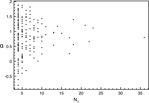
The other explanation for the lower experimental α values is artifactual. Single particle tracking generates a distribution of trajectory lengths limited by photo-bleaching, blinking, and trajectory crossings. The error in the MSD depends on the length of the trajectory N_T and the frame number n,³⁸ so we expect greater variance in Γ and α for short trajectories. For each experimental trajectory, we calculate the time averaged MSD and fit it up to n = 4 with Eq. 2. We used Eq. 2 because Δ_off in Eq. 5 was determined only for 0 ⩽ α ⩽ 1, and in this case the precise value of α is less important than the overall distribution. Figure 6 shows α versus the trajectory length for C=0.27. As expected, the variance in α is greatest for the shortest trajectories. For the shortest trajectories n = N_T = 4, it is even possible to get unphysical values of α < 0; short trajectories looping back to the starting position result in such a value, showing that analyzing MSDs with n ∼ N_T is meaningless.

Figure 6.

Distribution of experimental anomalous diffusion exponents at C=0.27 gel phase area fraction. N_T is the number of frames in a trajectory. There are 185 trajectories, the shortest are four frames in length and the longest 36 frames. α < 0 should be interpreted with caution; see text for discussion.

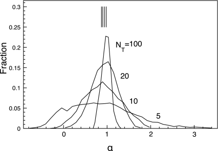
It is surprising that not only does the variance in α increase for short trajectories, the mean value systematically decreases. To show that this is not an experimental artifact, we cut the simulated trajectories into shorter, 5, 10, 20, and 100 step trajectories to match the timescale and statistics of the experimental trajectories. We coarsened the timescale, such that 1Δt in the new short trajectories is 9000 original Monte Carlo steps. We fit the time averaged MSD for the short trajectories up to n = 5 to Eq. 2. Figure 7 shows the α distribution for C=0.27. The distribution for low N_T is very broad and the mean has shifted to a lower value. The mean for N_T = 100 is $\overline{\alpha }=0.98$, close to the simulated value reported in Table 2 and for N_T = 5, $\overline{\alpha }=0.87$, close to the experimental value. The downshift in α even occurs in the unobstructed case.²⁴ Thus, systematically lower values of α in the experiments also stem from the predominance of short trajectories.

Figure 7.

Distributions of simulated α values for different trajectory lengths for obstacle area fraction C=0.27. α was obtained by a fit of Eq. 2 to the trajectory's MSD up to 5Δt. To match the statistics and timescale of the experiments, here 1Δt = 9000 simulation time steps. N_T is the length of trajectories in units of Δt. The vertical lines are the average values, $\overline{\alpha }$.

These results highlight the importance of the n∕N_T ratio when analyzing single molecule tracking data. It is critical when the magnitude of diffusion parameters are being used to classify trajectories or compare diffusion between different cells. For contrasting different modes of diffusion (e.g., for a certain cell type), either the same n∕N_T ratio should be used in both the cases or a classification scheme based on simulations³⁹ should be used.

Confinement models

Hop diffusion is a powerful model to describe obstructed diffusion in cell membranes.^{40, 41, 42} In many cell types, lipids and proteins diffuse in confined regions of 30-700 nm and then hop to a neighboring region with compartment size and residence time determined based on MSDs. Although our system (Fig. 1) does not resemble the classic fence and picket model, we can interpret our results in terms of hop diffusion as many of the same dynamic features are observed. The correlation length ξ in our system , which is in the range of 150-620 nm, is on the same scale as compartment sizes observed in cells.⁴³ The residence time in the hop diffusion model can be compared to the crossover time t_CR. Previous work has demonstrated the importance of time resolution in MSD data to understand the obstacle or confinement structure.^{41, 42, 44} With 35 ms time resolution in our experiments, we can observe the transition from anomalous to normal diffusion only for correlation lengths ξ > 600 nm. In the hop diffusion model, the residence time depends on the size of the confinement region and on the probability that the tracer crosses from one region to a neighbor. Similarly, t_CR depends on the correlation length ξ and the fractal dimension D_f of the fluid phase. Thus, D_f is analogous to the fence crossing probability as illustrated in Ref. 42 where a larger barrier makes the MSD more anomalous. Murase et al.⁴³ also found that oligimerization of DOPE enhanced confinement and attributed this to the increased interaction between the larger oligomer and the anchored membrane proteins. We expect a similar dependence on species size in our system, as percolation thresholds normally decrease with diffuser size.^{29, 45}

As our results can be interpreted both in terms of percolation or hop diffusion, we suggest analysis of MSD data such as in Fig. 5 as a universal method to probe obstacle structure. If data suggesting a particular structure is available, it should definitely be used to aid the analysis of diffusion data. In many cellular systems, the structure of obstacles is unknown and probably diverse.¹² Without any assumptions, the correlation length can be interpreted as the length scale of the obstructions in the system. To interpret the anomalous diffusion exponent, simulations may be helpful to estimate the fence crossing probability or fractal dimension.

Stochastic models

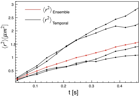
Related to the question of the underlying mechanism behind anomalous diffusion in cells is the question of the stochastic process. Several stochastic processes lead to anomalous diffusion, including percolation, fractional Brownian motion and the continuous-time random walk (CTRW).²¹ It has been demonstrated that single particle diffusion data can determine the underlying stochastic process.^{46, 47, 48} Lubelski et al. showed that the ergodicity breaking inherent to some CTRW processes, leads to different time-averaged and ensemble-averaged MSDs.⁴⁶ Therefore, we show (Fig. 8) the full ensemble-averaged and time-averaged MSDs for the four longest trajectories (N_T ⩾ 30) in the C = 0.59 sample. Even the longest experimental trajectories vary around the ensemble averaged MSD. We do not observe the large systematic decrease in transport coefficient for the time-averaged MSDs and trend toward α = 1 expected for a CTRW. Although the experimental trajectories are short compared to simulations, this suggests that we are not observing a CTRW with a power law distribution of waiting times. Our direct AFM data suggests a percolation type process, but in a system where the underlying mechanism is unknown, this could be a valuable piece of evidence.

Figure 8.

Ensemble-averaged MSD (red) and time-averaged MSD for the four longest trajectories (N_T ⩾ 30) (black) in the C=0.59 sample.

CONCLUSION

Single molecule tracking is a valuable tool to probe subdiffusive behavior of membrane constituents and thereby understand the organization of the plasma membrane. The challenge is to reveal the underlying mechanisms causing anomalous subdiffusion. We have presented an experimental system where single molecule tracking quantifies the subdiffusion and concurrently AFM images the obstacles. Our results demonstrate the opportunities and limitations of using single molecule tracking data to deduce the obstacle structure. We believe that the greatest challenge in single molecule tracking is to measure over long times, as short trajectories (N_T < 10) can lead to erroneous predictions of the anomalous diffusion exponent. Limited temporal range also limits the length scale of obstacles that can be detected as a transition from anomalous to normal diffusion. The typical single molecule resolution of 35 ms allows observation of a transition for ξ ⩾ 620 nm. Without better data, it will be difficult to apply more advanced statistics to discriminate between various stochastic processes driving anomalous subdiffusion.

References

- Anderson C. M., Georgiou G. N., Morrison I. E. G., Stevenson G. V. W., and Cherry R. J., J. Cell Sci. 101, 415 (1992). [DOI] [PubMed] [Google Scholar]
- Saxton M. J. and Jacobson K., Annu. Rev. Biophys. 26, 373 (1997). 10.1146/annurev.biophys.26.1.373 [DOI] [PubMed] [Google Scholar]
- Schütz G. J., Kada G., Pastushenko V. Ph., and Schindler H., EMBO J. 19, 892 (2000). 10.1093/emboj/19.5.892 [DOI] [PMC free article] [PubMed] [Google Scholar]
- Smith P., Morrison I., Wilson K., Fernández N., and Cherry R., Biophys. J. 76, 3331 (1999). 10.1016/S0006-3495(99)77486-2 [DOI] [PMC free article] [PubMed] [Google Scholar]
- Lommerse P., Vastenhoud K., Pirinen N., Magee A., Spaink H., and Schmidt T., Biophys. J. 91, 1090 (2006). 10.1529/biophysj.105.079053 [DOI] [PMC free article] [PubMed] [Google Scholar]
- Ritchie K., Iino R., Fujiwara T., Murase K., and Kusumi A., Mol. Membr Biol. 20, 13 (2003). 10.1080/0968768021000055698 [DOI] [PubMed] [Google Scholar]
- Guigas G. and Weiss M., Biophys. J. 94, 90 (2008). 10.1529/biophysj.107.117044 [DOI] [PMC free article] [PubMed] [Google Scholar]
- Dietrich C., Yang B., Fujiwara T., Kusumi A., and Jacobson K., Biophys. J. 82, 274 (2002). 10.1016/S0006-3495(02)75393-9 [DOI] [PMC free article] [PubMed] [Google Scholar]
- Chen Y., Thelin W., Yang B., Milgram S., and Jacobson K., J. Cell Biol. 175, 169 (2006). 10.1083/jcb.200512116 [DOI] [PMC free article] [PubMed] [Google Scholar]
- Saxton M. J., Biophys. J. 92, 1178 (2007). 10.1529/biophysj.106.092619 [DOI] [PMC free article] [PubMed] [Google Scholar]
- Douglass A. and Vale R., Cell 121, 937 (2005). 10.1016/j.cell.2005.04.009 [DOI] [PMC free article] [PubMed] [Google Scholar]
- Nicolau D., Hancock J., and Burrage K., Biophys. J. 92, 1975 (2007). 10.1529/biophysj.105.076869 [DOI] [PMC free article] [PubMed] [Google Scholar]
- Kam L., J. Struct. Biol. 168, 3 (2009). 10.1016/j.jsb.2009.05.006 [DOI] [PMC free article] [PubMed] [Google Scholar]
- Ratto T. V. and Longo M. L., Biophys. J. 83, 3380 (2002). 10.1016/S0006-3495(02)75338-1 [DOI] [PMC free article] [PubMed] [Google Scholar]
- Chan Y. and Boxer S., Curr. Opin. Chem. Biol. 11, 581 (2007). 10.1016/j.cbpa.2007.09.020 [DOI] [PMC free article] [PubMed] [Google Scholar]
- Yu C. and Groves J., Med. Biol. Eng. Comput. 48, 1 (2010). 10.1007/s11517-010-0634-x [DOI] [PMC free article] [PubMed] [Google Scholar]
- Sanabria H., Kubota Y., and Waxham M., Biophys. J. 92, 313 (2007). 10.1529/biophysj.106.090498 [DOI] [PMC free article] [PubMed] [Google Scholar]
- Banks D. and Fradin C., Biophys. J. 89, 2960 (2005). 10.1529/biophysj.104.051078 [DOI] [PMC free article] [PubMed] [Google Scholar]
- Feder T. J., Brust-Mascher I., Slattery J. P., Baird B., and Webb W. W., Biophys. J. 70, 2767 (1996). 10.1016/S0006-3495(96)79846-6 [DOI] [PMC free article] [PubMed] [Google Scholar]
- Bouchaud J. and Georges A., Phys. Rep. 195, 127 (1990). 10.1016/0370-1573(90)90099-N [DOI] [Google Scholar]
- Havlin S. and Ben-Avraham D., Diffusion and Reactions in Fractals and Disordered Systems (Cambridge University Press, Cambridge, United Kingdom, 2000). [Google Scholar]
- Havlin S. and Ben-Avraham D., Adv. Phys. 36, 695 (1987). 10.1080/00018738700101072 [DOI] [Google Scholar]
- Fractals and Disordered Systems, edited by Bunde A. and Havlin S., 2nd ed. (Springer-Verlag, Berlin, 1996). [Google Scholar]
- See suplementary material at http://dx.doi.org/10.1063/1.3596377E-JCPSA6-134-004122 for materials and methods, and additional text and figures.
- Goksu E., Vanegas J., Blanchette C., Lin W., and Longo M., Biochim. Biophys. Acta 1788, 254 (2009). 10.1016/j.bbamem.2008.08.021 [DOI] [PubMed] [Google Scholar]
- Frederix P. L. T. M., Bosshart P. D., and Engel A., Biophys. J. 96, 329 (2009). 10.1016/j.bpj.2008.09.046 [DOI] [PMC free article] [PubMed] [Google Scholar]
- Johnston L., Langmuir 23, 5886 (2007). 10.1021/la070108t [DOI] [PubMed] [Google Scholar]
- Saxton M. J., Biophys. J. 61, 119 (1992). 10.1016/S0006-3495(92)81821-0 [DOI] [PMC free article] [PubMed] [Google Scholar]
- Saxton M. J., Biophys. J. 64, 1053 (1993). 10.1016/S0006-3495(93)81471-1 [DOI] [PMC free article] [PubMed] [Google Scholar]
- Kiessling V., Crane J. M., and Tamm L. K., Biophys. J. 91, 3313 (2006). 10.1529/biophysj.106.091421 [DOI] [PMC free article] [PubMed] [Google Scholar]
- Deverall M. A., Gindl E., Sinner E. K., Besir H., Ruehe J., Saxton M. J., and Naumann C. A., Biophys. J. 88, 1875 (2005). 10.1529/biophysj.104.050559 [DOI] [PMC free article] [PubMed] [Google Scholar]
- Schütz G., Schindler H., and Schmidt T., Biophys. J. 73, 1073 (1997). 10.1016/S0006-3495(97)78139-6 [DOI] [PMC free article] [PubMed] [Google Scholar]
- Matsuoka S., Shibata T., and Ueda M., Biophys. J. 97, 1115 (2009). 10.1016/j.bpj.2009.06.007 [DOI] [PMC free article] [PubMed] [Google Scholar]
- Martin D. S., Forstner M. B., and Käs J. A., Biophys. J. 83, 2109 (2002). 10.1016/S0006-3495(02)73971-4 [DOI] [PMC free article] [PubMed] [Google Scholar]
- Goulian M. and Simon S., Biophys. J. 79, 2188 (2000). 10.1016/S0006-3495(00)76467-8 [DOI] [PMC free article] [PubMed] [Google Scholar]
- Wieser S., Moertelmaier M., Fuertbauer E., Stockinger H., and Schütz G., Biophys. J. 92, 3719 (2007). 10.1529/biophysj.106.095398 [DOI] [PMC free article] [PubMed] [Google Scholar]
- Saxton M. J., Biophys. J. 66, 394 (1994). 10.1016/S0006-3495(94)80789-1 [DOI] [PMC free article] [PubMed] [Google Scholar]
- Qian H., Sheetz M. P., and Elson E. E., Biophys. J. 60, 910 (1991). 10.1016/S0006-3495(91)82125-7 [DOI] [PMC free article] [PubMed] [Google Scholar]
- Kusumi A., Sako Y., and Yamamoto M., Biophys. J. 65, 2021 (1993). 10.1016/S0006-3495(93)81253-0 [DOI] [PMC free article] [PubMed] [Google Scholar]
- Kusumi A., Nakada C., Ritchie K., Murase K., Suzuki K., Murakoshi H., Kasai R. S., Kondo J., and Fujiwara T., Annu. Rev. Biophys. Biomol. Struct. 34, 351 (2005). 10.1146/annurev.biophys.34.040204.144637 [DOI] [PubMed] [Google Scholar]
- Ritchie K., Shan X., Kondo J., Iwasawa K., Fujiwara T., and Kusumi A., Biophys. J. 88, 2266 (2005). 10.1529/biophysj.104.054106 [DOI] [PMC free article] [PubMed] [Google Scholar]
- Niehaus A. M.S., Vlachos D. G., Edwards J. S., Plechac P., and Tribe R., Biophys. J. 94, 1551 (2008). 10.1529/biophysj.107.106484 [DOI] [PMC free article] [PubMed] [Google Scholar]
- Murase K., Fujiwara T., Umemura Y., Suzuki K., Iino R., Yamashita H., Saito M., Murakoshi H., Ritchie K., and Kusumi A., Biophys. J. 86, 4075 (2004). 10.1529/biophysj.103.035717 [DOI] [PMC free article] [PubMed] [Google Scholar]
- Saxton M. J., Biophys. J. 69, 389 (1995). 10.1016/S0006-3495(95)79911-8 [DOI] [PMC free article] [PubMed] [Google Scholar]
- Saxton M. J., Biophys. J. 99, 1490 (2010). 10.1016/j.bpj.2010.06.033 [DOI] [PMC free article] [PubMed] [Google Scholar]
- Lubelski A., Sokolov I., and Klafter J., Phys. Rev. Lett. 100, 250602 (2008). 10.1103/PhysRevLett.100.250602 [DOI] [PubMed] [Google Scholar]
- Szymanski J. and Weiss M., Phys. Rev. Lett. 103, 038102 (2009). 10.1103/PhysRevLett.103.038102 [DOI] [PubMed] [Google Scholar]
- Tejedor V., Bénichou O., Voituriez R., Jungmann R., Simmel F., Selhuber-Unkel C., Oddershede L., and Metzler R., Biophys. J. 98, 1364 (2010). 10.1016/j.bpj.2009.12.4282 [DOI] [PMC free article] [PubMed] [Google Scholar]