Modeling and automation of sequencing-based characterization of RNA structure

Abstract

Sequence census methods reduce molecular measurements such as transcript abundance and protein-nucleic acid interactions to counting problems via DNA sequencing. We focus on a novel assay utilizing this approach, called selective 2′-hydroxyl acylation analyzed by primer extension sequencing (SHAPE-Seq), that can be used to characterize RNA secondary and tertiary structure. We describe a fully automated data analysis pipeline for SHAPE-Seq analysis that includes read processing, mapping, and structural inference based on a model of the experiment. Our methods rely on the solution of a series of convex optimization problems for which we develop efficient and effective numerical algorithms. Our results can be easily extended to other chemical probes of RNA structure, and also generalized to modeling polymerase drop-off in other sequence census-based experiments.

Over the past 30 years, techniques have been developed that probe RNA structures with small molecules. In this class of techniques, a chemical reagent modifies RNA molecules in a structure-dependent fashion. Depending on the reagent used, four distinct types of information can be gleaned, including spatial nucleotide contact information, solvent accessibility of the RNA backbone, the local electrostatic environment adjacent to each nucleotide, and the local nucleotide flexibility (1). In each of these techniques, the modification location is detected during conversion to cDNA by blockage of reverse transcriptase at the modification site (Fig. 1). The detection can be performed by direct sequencing of the cDNA fragments using high-throughput sequencing technology (2). However, because at most a single modified site is revealed by every sequenced fragment (the closest modification to the 3′ end), a mathematical model and inference framework are needed to accurately infer the underlying structural properties given the observed fragment distribution.

Fig. 1.

Overview of SHAPE-Seq. As the reverse transcriptase (blue oval) transcribes the RNA, it encounters the first adduct and drops off (Left), or may drop off prematurely (Right). Sequencing of fragments produces data in the form of fragment counts (X). Similarly, a control experiment (Right) measures natural drop-off (fragments labeled Y). The model parameters consist of the adduct probabilities (Θ), the Poisson rate for the number of adducts per molecule (c), and the drop-off probabilities in the control experiment (Γ). Their estimates are denoted by Θ^⋆, Γ^⋆, and c^⋆.

In this work, we introduce such a model and framework in the context of the SHAPE (selective 2′-hydroxyl acylation analyzed by primer extension) technique for characterizing local nucleotide flexibility (3–5). The identification of adduct formation can be performed by capillary electrophoresis (SHAPE-CE) or by high-throughput sequencing of cDNA fragments (SHAPE-Seq) (2) (Fig. 1). Every fragment begins at the 3′ end of the molecule and terminates at some adduct [(+) channel], or possibly at a location where there was natural polymerase drop-off (6, 7), which is controlled for in a separate control experiment [(−) channel]. Following sequencing, reads are mapped back to the RNA sequence and are classified by their end location. The resulting read counts are the sufficient statistics for a model that is used to infer estimates of the probabilities of adduct formation at each nucleotide, called relative reactivities.

The probabilistic model we develop for SHAPE and the sequencing that follows in SHAPE-Seq is highly structured and has recursive properties that allow for efficient maximum-likelihood inference and confidence interval estimates. Our approach is inspired by probabilistic models used in RNA sequencing (RNA-Seq) analysis to measure transcript identity and abundance (8) and should be easily generalizable to any chemical probing technique that characterizes different aspects of RNA structure. We present results that confirm the accuracy of our approach and that reveal the simplicity in analyzing the data despite the complexity of the models. Together, these provide a proof of principle for the utilization of SHAPE-Seq for high-throughput RNA structure characterization.

Modeling Polymerase Drop-Off

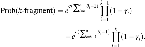
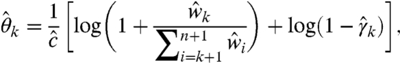
We consider an RNA molecule that contains n sites. The sites are numbered 1 to n according to their sequence position with respect to the molecule’s 3′ end, where the latter is assigned position 0 and is excluded from analysis (Fig. 1). In a SHAPE-Seq experiment, we observe cDNA fragments of varying lengths, where a k-fragment corresponds to a mapped read of length k that spans sites 0 to k - 1 (1 ≤ k ≤ n), and a complete fragment corresponds to a full transcript of length n + 1. In the (−) channel control assay, the primary source of incomplete fragments is reverse transcriptase’s (RT) natural drop-off while transcribing the molecule. Natural drop-off arises largely due to structural properties of the molecule, and thus RT’s propensity to drop may vary along sites. To study this process at nucleotide resolution, we define the drop-off propensity at site k, γ_k, to be the conditional probability that RT terminates transcription at site k, given that it has reached this site. The n parameters Γ = (γ₁,…,γ_n), 0 ≤ γ_k ≤ 1 ∀ k, completely characterize natural drop-off, and we wish to estimate them from the (−) channel fragment counts.

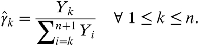
A maximum-likelihood (ML) estimate of Γ is derived from the (−) channel k-fragment and complete fragment counts (Y₁,…,Y_n+1) as follows: We denote by p_k the probability that a molecule results in a k-fragment (1 ≤ k ≤ n) and by p_n+1 the probability that it is transcribed in full. The likelihood of the counts is thus proportional to , where 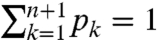, and takes the form of a log linear model. It is well-known that such a model is uniquely maximized by

[1]

from which we can retrieve the estimate using the relations for k = 1,…,n. We obtain γ_k by observing that a fragment has length greater than k if and only if no drop-off occurred until site k; that is, . Hence,

[2]

Importantly, RT’s drop-off gradually degrades the pool of actively transcribed molecules throughout the experiment and is captured by the relations .

Modeling Chemical Modification

In the (+) channel, the RNA is treated with an electrophile that reacts with conformationally flexible nucleotides to form 2′-O-adducts. We define the relative reactivity of a site to be the probability of adduct formation at that site. Therefore, associated with the RNA molecule are n nonnegative real numbers Θ = (θ₁,…,θ_n), , which we wish to estimate from sequencing data.

During modification, an RNA may be exposed to variable numbers of electrophile molecules. We model the number of times an RNA is exposed to electrophile molecules as a Poisson process of an unknown rate c > 0, i.e., we assume that

[3]

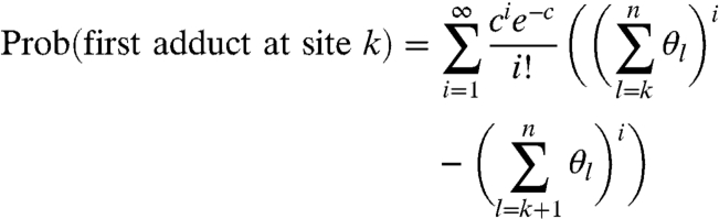
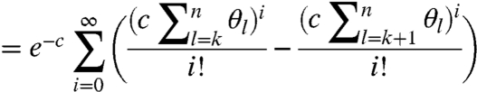
where each exposure may result in the modification of a site. A point that is key to interpreting SHAPE data is that a k-fragment is assumed to be generated when site k is the site that is first encountered by RT, regardless of the number of adducts that formed upstream of k. This is important in light of the fact that SHAPE experiments are calibrated to yield single-hit kinetics (i.e., c ≈ 1). Under such conditions, a considerable portion of the molecules are hit twice or more (e.g., 26.42% when c = 1, as compared to 36.79% that are hit once). Given that an RNA is exposed i times, the probability that a molecule carries its first adduct at site k is

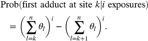[4]

When k = n, the second sum is taken to be 0 so that Eq. 4 reduces to (for convenience, we define 0⁰ = 1). Note that Eq. 4 entails an approximation to our understanding of SHAPE chemistry as it allows for repeated modification of a site. This approximation is minor, however, largely due to negligible abundance of molecules with a multitude of adducts under single-hit kinetics as well as the lengths of the molecules. This premise is also supported by robustness analysis of our framework (see SI Text for details). Notably, the low probability of many hits also justifies the use of an unbounded Poisson model rather than its truncation.

We can now obtain the probability of a molecule being modified at site k (although possibly also at subsequent sites):

[5]

[6]

[7]

Incorporating the natural drop-off probabilities, we have

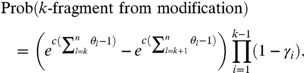[8]

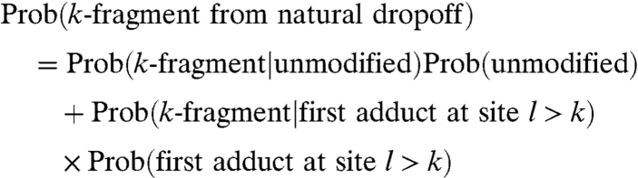
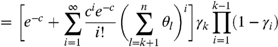
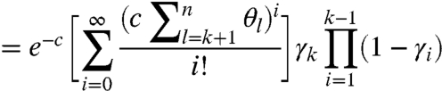
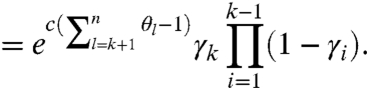
where reflects the natural degradation in the elongating modified-molecule pool. We attribute all other observed fragments to natural causes, which take effect in two distinct pools: unmodified molecules and modified ones for which RT may drop off before encountering the first adduct (see Fig. 1). These factors are combined to yield the probability of observing a k-fragment from natural drop-off:

[9]

[10]

[11]

[12]

As a special case, the probability of observing a complete fragment in the (+) channel is

[13]

It can be seen from Eqs. 10 and 13 that under single-hit kinetics, the unmodified pool is expected to occupy a significant portion of the target pool, as c = 1 implies equal probabilities of experiencing no modification or a single hit. We can think of it as having a (−) channel contained within the (+) channel. Finally, based on Eqs. 8–12, the probability of observing a k-fragment in the (+) channel is

[14]

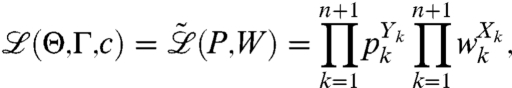
Assuming we observe (X₁,…,X_n+1) k-fragment and complete fragment counts in the (+) channel, the likelihood of observing the entire data from both channels is given by

[15]

and can be explicitly written as

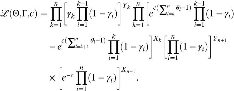[16]

Here, we maximize 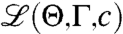to find the model parameters that best explain the observed data and thus best reflect underlying structural properties of the RNA molecule.

Maximum-Likelihood Estimation

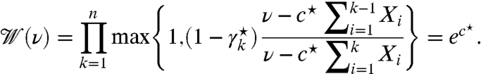
We begin by stating a theorem that leads to an algorithm for ML estimation which either provides the exact solution, or else fails and reports that status. We assume that X_n+1,Y_n+1 > 0.

Algorithm 1:

1. Estimate c by setting

   [17]
2. Estimate Γ by setting

   [18]
3. Estimate the SHAPE reactivities Θ by

   [19]

   where describe the observed (+) channel fragment-length distribution; i.e., .

Thoerem 1.

If Eqs. 17–19 yield for all 1 ≤ k ≤ n and , then they determine the parameters that uniquely maximize the likelihood Eq. 16 over all distributions Θ, over Γ such that 0 ≤ γ_k ≤ 1, and over .

Proof:

We first cast Eq. 16 as the following simplified log linear model:

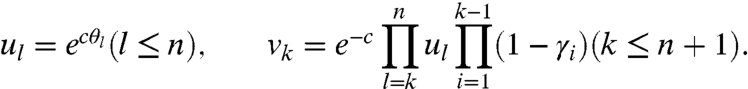
[20]

where the p_k’s were defined earlier, w_k = Prob(k-fragment) (1 ≤ k ≤ n), and w_n+1 = Prob(complete fragment) as in Eqs. 13 and 14. To simplify notation, we define the variables

[21]

Note that Eqs. 13 and 14 imply w_k = v_k - v_k+1 (1 ≤ k ≤ n) and w_n+1 = v_n+1, and that setting results in v₁ = 1. Becuse the w_k’s represent probabilities, they are nonnegative and hence the v_k’s form a weakly decreasing sequence . It is now also easy to see that because the sum is telescoping.

We can now leverage well-known results for ML estimation of log linear models. Essentially, when the parameters are nonnegative and sum to a known constant there is a unique closed-form ML solution (9). The model in Eq. 20, however, imposes two constraints: 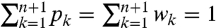. In this case, similar techniques (i.e., Lagrange multipliers) can be used to show that the likelihood is uniquely maximized by

[22]

A direct consequence of Eq. 22 is that can be determined from , as was done earlier (see Eq. 2). One can also resolve from because implies . To backtrack , we use the previous construction: from the definitions we have that , and hence

[23]

Now, from Eq. 21 we have and therefore

[24]

Eq. 19 then follows from .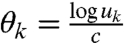

It is left to verify whether the obtained solution lies within the problem’s domain. Clearly, the ’s are properly bounded, and our construction also guarantees whenever (via and Eq. 21). However, Eq. 17 might result in , which is indicative of problematic data. More importantly, it is possible to encounter jointly with (or ) for some k’s. To observe this, consider the product in Eq. 24: The right-hand factor equals at most 1, whereas the left-hand factor equals at least 1. Yet, both factors are based on data from the (+) and (−) channels and are not constrained to guarantee that , thereby leading to cases where and or . In such cases, Eq. 20’s solution maps to an infeasible parameter set.

Theorem 1 states that Algorithm 1 fails if the estimates are negative, as the results are then not biologically meaningful. Intuitively, negative reactivities arise when the frequencies of certain k-fragments in the (+) channel are exceedingly low compared to their (−) channel counterparts, to the extent that they cannot be explained by setting the relevant ’s to zero. In general, negative reactivities indicate that the (+) channel data are inconsistent with the (−) channel data, or in other words, that the entire dataset is “too noisy.”

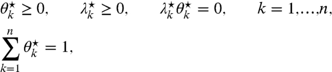
When the user wishes to proceed with analysis in the presence of data inconsistencies (see Interpretation), our goal is to resolve them by finding 2n + 1 feasible parameters that maximize Eq. 16. Notably, optimizing the function efficiently is particularly important since SHAPE-Seq is geared toward highly multiplexed probing (2). This, in turn, necessitates rapid analysis of the data collected from a multitude of distinct RNA molecules. Nevertheless, efficient optimization is computationally challenging for the following reasons. First, it involves boundary and fixed-sum constraints, which preclude the use of standard local optimization methods (e.g., gradient-based algorithms). Second, its scale is large, as n is typically on the order of several hundreds (3, 7). Here, we present Algorithm 2, which provides an efficient numerical solution despite the problem’s complexity and large dimension. Note that hereafter we explicitly require .

Algorithm 2:

1. Initialize. Exclude from analysis all entries where X_k = Y_k = 0. For each of the remaining n^′ entries, use Algorithm 1’s output to set and .

2. If increased in less than ϵ or if M iterations were completed then stop, else solve the following three optimization problems:

   • Optimize for c. Find c > 0 that maximizes . Set c^⋆ to the solution.
   • Optimize for Γ. Find Γ that maximizes under the constraints 0 ≤ γ_k ≤ 1 (k ≤ n^′). Set Γ^⋆ to the solution.
   • Optimize for Θ. Find Θ that maximizes under the constraints θ_k≥0 (k ≤ n^′), . Set Θ^⋆ to the solution.

Go to step 2.

The advantage to this formulation is that each of the three subproblems is a convex optimization problem, as established by Lemmas 1–3 in SI Text. A convex optimization problem has two attractive properties: (i) if a local maximum exists, it is a global maximum, and (ii) it is, in general, numerically tractable via specialized interior-point methods (10). Yet, we stress that these methods’ tractability and accuracy are limited by the problem’s dimension and also depend to a large extent on its structure. We circumvent these deficiencies by obtaining exact solutions for the high-dimensional coordinate problems, namely maximizing Θ and Γ, as stated in the next two theorems.

Theorem 2.

Given c^⋆ > 0 and a distribution Θ^⋆, the likelihood function attains a unique maximum over all Γ∈[0,1]ⁿ at that is the maximum of zero and

[25]

for all 1 ≤ k ≤ n, where (0 ≤ k ≤ n) and (1 ≤ k ≤ n).

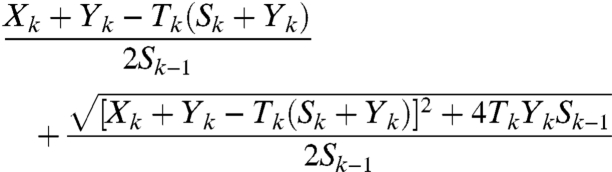
The proof of the Theorem is in SI Text.

Although the third problem is not amenable to an explicit solution like the second one, the next theorem shows that it can in fact be reduced to numerically solving an equation in one variable. Here, we utilized the water filling optimization technique, which has been previously used to optimize power-constrained transmission over parallel Gaussian channels (11). A sketch of the proof is included below, with full details in SI Text.

Theorem 3.

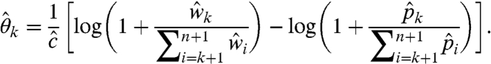
Given c^⋆ > 0 and Γ^⋆∈[0,1]ⁿ, the likelihood function has a unique maximum over all distributions Θ, given by that is the maximum of zero and

[26]

for all 1 ≤ k ≤ n, where solves the piecewise equation

[27]

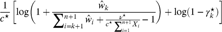
Outline of proof:

The Karush–Kuhn–Tucker (KKT) constraints are a set of conditions that are necessary and sufficient for the optimality of a solution of a convex optimization problem with inequality constraints (10). We derive them by introducing a Lagrange multiplier, denoted ν^⋆, which corresponds to the fixed-sum constraint, and n KKT multipliers, denoted , which pertain to the nonnegativity constraints. Using these variables, we obtain the following conditions:

[28]

[29]

where is the derivative of .

Next, we derive the relations between , , and ν^⋆ that solve Eq. 29 for a site k. First, assume that it is solvable for , in which case we set . The left-hand side of Eq. 29 then becomes the sum of a nonnegative constant and a strictly monotonously decreasing function that is illustrated in Fig. S1A. The choice of ν^⋆ thus completely (and explicitly) determines , but importantly, ν^⋆ must be smaller than a certain threshold to yield . This threshold depends on the constants c^⋆, X₁,…,X_k, and and thus varies among the n sites. When ν^⋆ exceeds site k’s threshold, the resulting violates the nonnegativity constraint and instead we set it to zero and use as a slack variable to fill the gap between ν^⋆ and .

The derived relations imply that given ν^⋆, a subset of Θ^⋆’s entries may be set to zero, with the remaining entries being determined from ν^⋆ via Eq. 26. Furthermore, the subset’s cardinality decreases as we decrease ν^⋆ and gradually cross the thresholds of additional sites, where their ’s become positive. Having obtained an explicit expression for , it is left to find the ν^⋆ at which . It is found by observing that 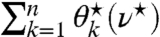forms a piecewise continuous and strictly monotonously decreasing function (with increasing ν^⋆), with breakpoints at the above-mentioned thresholds, where the zero-entry subset is updated. Note that the monotonicity between breakpoints is due to ’s strict monotonicity, whereby expands as ν^⋆ decreases. This allows us to gradually decrease ν^⋆ until the sum reaches 1 and can be visualized as flooding a region of varying surface levels up to a constant amount of water (see Fig. S1B). The original problem thereby reduces to finding the intersection of with 1, or alternatively, of 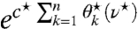with e^c⋆, as formulated in Eq. 27.

Despite the apparent complexity of Eq. 27, its special properties lead to a straightforward root-finding routine. This, coupled with efficient methods to solve the first two optimization problems (see SI Text), enabled us to implement Algorithm 2 so that it can be run for hundreds of RNA molecules in a matter of minutes (2).

Results

We used our automated bioinformatics pipeline to analyze data from SHAPE-Seq probing of a mixture of well-studied RNAs of lengths n = 172–198. Alignments were generated by mapping sequenced fragments to the known RNA sequences using the Bowtie paired-end alignment program (12).

ML estimation took 1–2 s per molecule on a personal computer, and the reconstructed reactivities were in very good agreement with those obtained from SHAPE-CE probing and analysis (2). An example is shown in Fig. 2 for the Staphylococcus aureus plasmid pT181 sense RNA. The raw k-fragment frequencies in the (+) channel are illustrated next to the outputs of Algorithms 1 and 2. The estimated rate was . One can readily observe the input signal’s decay as well as a general trend in its reconstruction, that is, signal attenuation at the molecule’s 3′ end gradually transitions into amplification over its 5′ end. Additionally, Algorithm 1’s intermediate output is indicative of high-quality data, as it displays very few negative estimates. The depicted error bars correspond to one standard deviation of 500 bootstrap samples of the dataset and indicate negligible variation. The complete details of estimation results and subsequent structural analysis conducted for all probed molecules appear in ref. 2. The full data analysis pipeline is available at http://bio.math.berkeley.edu/SHAPE-Seq/ as a supplementary file for download (see SI Text for details).

Fig. 2.

ML estimation for S. aureus plasmid pT181 sense RNA. Bootstrap error bars are shown in black on the final ML estimation. Sites 1–45 showed negligible frequencies and were omitted from display. The starred bar is not fully shown and has magnitude -0.16.

To explore the robustness of our method, we investigated the accuracy of the estimated Θ as a function of the sequencing depth as well as under several model scenarios featuring hypothetical Θ and Γ distributions. We assessed robustness with respect to data size by analyzing, for different sizes, 200 randomly drawn subsets of our dataset and determining the fraction of sites that were assigned reactivities within 15% of the full-dataset estimate. Average fraction and sample variation per subset size are shown in Fig. S2. They demonstrate that high quality is retained in the presence of an order-of-magnitude decrease in data throughput and that a decrease of two orders of magnitude results in fair accuracy. Fig. S3 recapitulates the latter claim by demonstrating that 0.5% of the reads suffice to capture the general reactivity profile of our dataset. The dependence of estimation quality on structural features of the RNA was assessed by assigning various distributions to Θ and Γ and subsequently drawing 5 million fragments from the induced fragment distributions. We collected 15%-, 10%-, and 5%-interval statistics. For 500 simulations per case, the average fraction of hits decreased with increasing number of reactive sites and was lowest for the extreme case of an exponentially declining Θ (i.e., 76% of 50 reactive sites were within the 5% interval). Yet, variation around the average was consistently negligible. In addition, effects of instantaneous drop-off spikes in Γ amounted to several percents degradation at the most. The complete analysis details are found in the SI Text and in Tables S1 and S2.

Interpretation

Although Algorithm 1 may fail to generate the ML solution, it is valuable in two ways. First, it informs the user of the experiment and data quality via and summary-level statistics such as , , and , which are not obtainable with the present SHAPE-CE pipeline (4). The extent of data inconsistencies is manifested in the negative ’s and can be assessed by inspecting their magnitudes and abundance. In the presence of large-magnitude negatives, the user may merely exclude certain sites from further analysis (e.g., structure prediction), as is commonly done in SHAPE-CE data analysis (4, 5).

Second, our model-based correction formula elucidates the effects of the two bias sources and guides how to offset them. This, in turn, highlights the virtues and deficiencies of existing bioinformatics approaches. Specifically, we can rewrite Eq. 19 such that it maps the input fragment-length distributions to the corrected output distribution, as follows:

[30]

One can see that the correction can be applied separately to the noisy signal component (i.e., left-hand term) and the noise component (i.e., right-hand term), as is currently done in SHAPE-CE (6). More importantly, each frequency is corrected according to its position in the distribution (i.e., its percentile). Particularly, we can approximate the correction factor by because, in general, 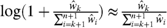when n is large. Amplification is thus adjusted according to the empirical cumulative distribution. This is in contrast to existing approaches where users apply a heuristic exponential-decay correction that corrects according to a nucleotide’s sequence position rather than its percentile (6, 7). Moreover, this correction’s range and parameters are chosen by the user, based on visual inspection.

In the ideal case where and γ_k = γ₀ ∀ k, the two approaches coincide (see illustration in Fig. S4A), whereas they differ as the RNA diverges from a uniform pattern, which is the case for biologically relevant RNAs. For example, in the Bacillus subtilis RNase P RNA specificity domain, most reactive bases are confined to a short segment (13), thereby inducing considerable signal decay over that region. However, due to its short span, it is easily missed by the eye (see SHAPE-Seq data in Fig. S4 B and C). The need for correction is also commonly overlooked in the (−) channel, which often displays a few outstanding spikes over low-frequency background. These reflect natural transcription barriers that significantly degrade the pool of molecules that are transcribed past these points. Hence, the decay pattern clearly departs from a smooth gradual decline toward a stepwise behavior, as illustrated in Fig. S4 D and E. Sharp instantaneous degradations in the target pool should be accounted for such that noise estimates past these points are boosted accordingly. In Eq. 30, this is encapsulated into the noise correction term, such that the spike’s effect is propagated to upstream sites, whereas existing methods merely subtract the spike locally from the matching signal intensity.

Finally, the above interpretation gives rise to a simple nonparametric correction, where logarithms are removed and reactivities are normalized such that . Interestingly, the reactivities reconstructed with this approach were, for the most part, very close to the ML estimates. However, they tend to diverge as reactivities increase, which, in turn, may confer more sensitivity to outliers.

Discussion

In this work, we present the first rigorous model of the SHAPE experiment used to probe the structures of RNA molecules. Using this model, we developed a robust method to determine the set of reactivities that best explains the observed cDNA fragment-length distribution. Coupled with our alignment pipeline, this produces an automated workflow for SHAPE analysis via sequencing and improves upon existing approaches for analyzing SHAPE data. Current approaches use a heuristic exponential decay correction and (−) channel scaling to assign low reactivities to user-identified sites thought to have little reactivity (6). Although they do correct for natural polymerase drop-off, these procedures can require expert knowledge to choose when and where to apply. Our approach also leverages accurate measurement of the number of full-length transcripts to provide an estimate of the modification rate, c. This has not been possible with SHAPE-CE due to detection limitations of CE in quantifying the signal of full-length fragments. Although our ML framework was applied to data generated from sequencing experiments, it could be adapted to CE-based data to automate their analysis.

Our robustness analysis shows that SHAPE-Seq is remarkably accurate even at low throughput making it tractable with lower throughput desktop sequencers, suitable for low abundance RNAs, and effective for multiplexed bar coding to simultaneously probe large numbers of molecules in parallel (2).

In the present work, we have focused on the application of our method to SHAPE-Seq (2). However, our method for modeling the effects of RT drop-off is broadly applicable to any sequence census method that utilizes a pool of RNA molecules as the basis for the measurement. In particular, our method should be directly applicable to the general class of RNA structure-dependent chemical probing techniques that utilize single modifications to probe other features such as solvent accessibility of the backbone and local electrostatic environment of the nucleotide (1). Additional interesting challenges will arise when extending our method to techniques where adduct formation is correlated to structural features at more than one position in the RNA, for example with chemicals that probe through-space neighbors (1). Other methods that involve converting RNA into cDNA, including transcript abundance quantitation and alternative splicing isoform identification with RNA-Seq (8, 14), and qRT-PCR, could potentially benefit from our estimation of premature termination of the RT process represented by to correct for drop-off biases. Moreover, we believe these methods generalize to the setting of random priming where fragments may not always begin at the same place, allowing us to determine the structures of de novo pools of RNA such as natural transcriptomes.

In general, our automated data analysis pipeline, coupled with the SHAPE-Seq protocol, is a high-throughput method to infer secondary and tertiary structural information for every nucleotide in an RNA solution (2). Furthermore, the final output of this method, the optimal Θ that represent the reactivity of each nucleotide to adduct formation, are well understood and can be used to constrain existing RNA structure prediction programs to remarkably increase their accuracy (5, 15). SHAPE-Seq should also be able to provide much-needed information for recent algorithms that predict tertiary RNA structures from primary sequence (16).

References

- 1.Weeks KM. Advances in RNA structure analysis by chemical probing. Curr Opin Struct Biol. 2010;20:295–304. doi: 10.1016/j.sbi.2010.04.001. [DOI] [PMC free article] [PubMed] [Google Scholar]
- 2.Lucks JB, et al. Multiplexed RNA structure characterization with selective 2′-hydroxyl acylation analyzed by primer extension sequencing (SHAPE-Seq) Proc Natl Acad Sci USA. 2011 doi: 10.1073/pnas.1106501108. 10.1073/pnas.1106501108. [DOI] [PMC free article] [PubMed] [Google Scholar]
- 3.Wilkinson KA, Merino EJ, Weeks KM. Selective 2′-hydroxyl acylation analyzed by primer extension (SHAPE): Quantitative RNA structure analysis at single nucleotide resolution. Nat Protoc. 2006;1:1610–1616. doi: 10.1038/nprot.2006.249. [DOI] [PubMed] [Google Scholar]
- 4.Low JT, Weeks KM. SHAPE-directed RNA secondary structure prediction. Methods. 2010;52:150–158. doi: 10.1016/j.ymeth.2010.06.007. [DOI] [PMC free article] [PubMed] [Google Scholar]
- 5.Deigan KE, Li TW, Mathews DH, Weeks KM. Accurate SHAPE-directed RNA structure determination. Proc Natl Acad Sci USA. 2008;106:97–102. doi: 10.1073/pnas.0806929106. [DOI] [PMC free article] [PubMed] [Google Scholar]
- 6.Vasa SM, Guex N, Wilkinson KA, Weeks KM, Giddings MC. ShapeFinder: A software system for high-throughput quantitative analysis of nucleic acid reactivity information resolved by capillary electrophoresis. RNA. 2008;14:1979–1990. doi: 10.1261/rna.1166808. [DOI] [PMC free article] [PubMed] [Google Scholar]
- 7.Wilkinson KA, et al. High-throughput SHAPE analysis reveals structures in HIV-1 genomic RNA strongly conserved across distinct biological states. PLoS Biol. 2008;6:e96. doi: 10.1371/journal.pbio.0060096. [DOI] [PMC free article] [PubMed] [Google Scholar]
- 8.Trapnell C, et al. Transcript assembly and quantification by RNA-Seq reveals unannotated transcripts and isoform switching during cell differentiation. Nat Biotechnol. 2010;28:511–515. doi: 10.1038/nbt.1621. [DOI] [PMC free article] [PubMed] [Google Scholar]
- 9.Pachter L, Sturmfels B, editors. Algebraic Statistics for Computational Biology. Cambridge, UK: Cambridge Univ Press; 2005. [Google Scholar]
- 10.Boyd S, Vandenberghe L. Convex Optimization. Cambridge, UK: Cambridge Univ Press; 2004. [Google Scholar]
- 11.Cover TM, Thomas JA. Elements of Information Theory. 2nd Ed. Hoboken, NJ: John Wiley; 2006. [Google Scholar]
- 12.Langmead B, Trapnell C, Pop M, Salzberg SL. Ultrafast and memory-efficient alignment of short DNA sequences to the human genome. Genome Biol. 2009;10:R25. doi: 10.1186/gb-2009-10-3-r25. [DOI] [PMC free article] [PubMed] [Google Scholar]
- 13.Liang R, Kierzek E, Kierzek R, Turner DH. Comparisons between chemical mapping and binding to isoenergetic oligonucleotide microarrays reveal unexpected patterns of binding to the Bacillus subtilis RNase P RNA specificity domain. Biochemistry. 2010;49:8155–8168. doi: 10.1021/bi100286n. [DOI] [PMC free article] [PubMed] [Google Scholar]
- 14.Mortazavi A, Williams BA, McCue K, Schaeffer L, Wold B. Mapping and quantifying mammalian transcriptomes by RNA-Seq. Nat Methods. 2008;5:621–628. doi: 10.1038/nmeth.1226. [DOI] [PubMed] [Google Scholar]
- 15.Mathews DH, et al. Incorporating chemical modification constraints into a dynamic programming algorithm for prediction of RNA secondary structure. Proc Natl Acad Sci USA. 2004;101:7287–7292. doi: 10.1073/pnas.0401799101. [DOI] [PMC free article] [PubMed] [Google Scholar]
- 16.Kladwang W, Das R. A mutate-and-map strategy for inferring base pairs in structured nucleic acids: Proof of concept on a DNA/RNA helix. Biochemistry. 2010;49:7414–7416. doi: 10.1021/bi101123g. [DOI] [PubMed] [Google Scholar]
Associated Data
This section collects any data citations, data availability statements, or supplementary materials included in this article.