Modeling Three-Dimensional Chromosome Structures Using Gene Expression Data

Abstract

Recent genomic studies have shown that significant chromosomal spatial correlation exists in gene expression of many organisms. Interestingly, coexpression has been observed among genes separated by a fixed interval in specific regions of a chromosome chain, which is likely caused by three-dimensional (3D) chromosome folding structures. Modeling such spatial correlation explicitly may lead to essential understandings of 3D chromosome structures and their roles in transcriptional regulation. In this paper, we explore chromosomal spatial correlation induced by 3D chromosome structures, and propose a hierarchical Bayesian method based on helical structures to formally model and incorporate the correlation into the analysis of gene expression microarray data. It is the first study to quantify and infer 3D chromosome structures in vivo using expression microarrays. Simulation studies show computing feasibility of the proposed method and that, under the assumption of helical chromosome structures, it can lead to precise estimation of structural parameters and gene expression levels. Real data applications demonstrate an intriguing biological phenomenon that functionally associated genes, which are far apart along the chromosome chain, are brought into physical proximity by chromosomal folding in 3D space to facilitate their coexpression. It leads to important biological insight into relationship between chromosome structure and function.

1. INTRODUCTION

1.1 Gene Location and Transcriptional Regulation

Transcription, as the first step in gene expression, is critical in determining protein and enzyme abundance in a cell. Regulation of transcriptional activities of gene ensembles in a living genome is a fundamental biological problem. By effectively addressing it, one expects to uncover governing principles behind normal and pathological states of cells. Recent studies have shown that gene location on a chromosome plays a critical role in determining transcription profiles in both prokaryotes and eukaryotes (Willenbrock and Ussery 2004). Distinct patterns of subtle but coordinated expression changes across neighboring genes on a chromosome were observed in many organisms, including Escherichia coli (E. coli) (Jeong, Ahn, and Khodursky 2004), yeast (Cohen et al. 2000; Kruglyak and Tang 2000), worm (Roy et al. 2002), fly (Boutanaev et al. 2002; Spellman and Rubin 2002), mouse (Li, Lee, and Zhang 2005), and human (Caron et al. 2001; Versteeg et al. 2003; Yager et al. 2004). For example, Cohen et al. (2000) discovered spatial correlation between adjacent genes along a chromosome in yeast expression. Képès (2003, 2004) revealed periodic epi-organization of the E. coli and yeast genomes by studying the distribution of transcriptional binding sites. Jeong, Ahn, and Khodursky (2004) demonstrated periodic patterns in E. coli expression using spectral analysis. Furthermore, several oncogenomic studies have revealed periodic patterns in gene expression and their clinical relevance in gastric cancer (Aggarwal et al. 2005), gliomas (Turkheimer et al. 2006), and breast cancer (Hanin et al. 2009). These patterns are likely induced by three-dimensional (3D) chromosome structures (Narlikar, Fan, and Kingston 2002; Khorasanizadeh 2004; Aggarwal et al. 2005). Therefore, evaluating possible 3D chromosome structures and their roles in transcriptional regulation is essential for our understanding of the biology of a cell (e.g., Tsankova et al. 2007; Renthal and Nestler 2008) and will be the focus of this article.

1.2 Chromosome Structures

Chromosomes must be tightly packed to fit into a cell. For example, chromosomal DNA of E. coli is ~1500 microns long, while the length and diameter of the cylindrical bacterium is only 3 and 1 micron(s), respectively. In human cells, chromosomal DNA molecules are 19–73 thousand microns in length, while a typical nucleus is ~2 microns in diameter. Hence they must be compacted hundreds and thousands of times through some folding structures in order to fit inside the nucleus. Such structures are important for DNA replication and transcriptional regulation, but their dynamic details in organisms are largely unknown (Wright et al. 2007).

A chromosome is composed of a deoxyribonucleic acid (DNA) molecule and structural proteins. DNA segments that carry genetic information are called genes, while other DNA sequences are involved in regulation of gene expression and/or may have structural functions. A basic structure of DNA molecules is the well-known double helix of two intertwined strands of polynucleotides, about 2 nm in diameter and 3.4 nm in pitch (i.e., the vertical distance between two adjacent parts of the helix located on the same surface). The DNA of a prokaryote (cells without nuclei, e.g., E. coli) is organized into a nucleoid, a distinct dynamic structure maintained through interactions with abundant DNA binding proteins. Prokaryotic chromosomes are generally supercoiled, but the detailed organization of supercoiled structures and underlying mechanisms remain unclear. The DNA of an eukaryote (cells with nuclei, e.g., yeast, plants, and animals) is wrapped around nucleosomes, forming a complex chromatin. An eukaryotic chromosome has at least three levels of organization: (1) DNA wrapped around nucleosomes—the “beads-on-a-string” structures resulting in about six-fold compaction; (2) a condensed chromatin fiber consisting of nucleosomes, resulting in additional 40-fold compaction; (3) nuclear scaffold loops, contributing to the residual compaction. The first two levels, referred to as local chromosome organization, are on the scale of 0.1–1 kilobase pair (kb), and generally affect transcriptional activities of individual genes. The third level, chromosome looping, is the most complex and least understood part of chromosome structures. We refer to the organization of supercoiled loops in a prokaryotic cell or chromatin fiber loops in a eukaryotic nucleus as chromosome folding structures, which can bring linearly distant genes into a close physical proximity to facilitate their coregulation. In our study, spatial correlation in transcriptional activities will be used to probe chromosome structures. Since the correlation reflects the interaction among (linearly distant) genes, the proper scale of underlying structures is at the level of chromosome folding rather than local organization of the chromatin.

1.3 Need for Statistical Methodology

High-resolution imaging techniques used to study microscopic structures either have physical limitations or are too invasive to study chromosome structures in a living cell without disturbing its properties. Other experimental techniques, such as spatial mapping of neighborhoods and genes, are labor intensive and require further technological developments (Oliver and Misteli 2005). Nevertheless, recent research has shown that structural features of chromosome organization are reflected in functional properties of a chromosome, that is, transcriptional activities (Jeong, Ahn, and Khodursky 2004). Therefore, spatial correlation in transcriptional activities along the chromosome can be used as a fingerprint to infer possible 3D chromosome structures.

While coordinated regulation of linearly distant loci in 3D is now recognized as a widespread phenomenon, demonstrated across a spectrum of organismal complexities (Cooper 1999; Eichler and Sankoff 2003; Hurst, Pal, and Lercher 2004), it remains unclear which higher-order chromosomal structures, if any, are critical for establishing at least transient juxtaposition of linearly distant DNA segments in 3D space. Carpentier et al. (2005) reported periodic patterns in intergenetic distances of the E. coli genome and raised a hypothesis that helical structures be dynamically formed at certain regions of the chromosome during transcription. Wright et al. (2007) examined the chromosomal periodicity of evolutionarily conserved gene pairs in E. coli and also hypothesized a helix-like topology. They further pointed out that a helical chromosome structure may bring coregulated genes into a relative spatial proximity, on one face of the structure. Moreover, analysis of the problem of optimal packing of strings under the requirement of limited uniformity of the 3D structure offered an intriguing, general solution: the helical secondary conformation allows for maximum packing capacity (Maritan et al. 2000). Although the hypothesis of helical structures is sensible, more evidence is needed to further validate it; more importantly, there is still great uncertainty about the number and sizes of loops (i.e, the constituent elements of such putative hyper-structures). For example, the E. coli chromosome was originally postulated to have 12–80 topologically isolated loops (Worcel and Burgi 1972), and was refined by Sinden and Pettijohn (1981) to have 50 loops with domain size of ~100 kbs. Recently, Postow et al. (2004), Jeong, Ahn, and Khodursky (2004), and Carpentier et al. (2005) have shown evidence for the size of distinct topological domains on the order 10 kbs. Thus, analytical and computational approaches are needed to accurately infer the structural parameters. Further, chromosome spatial patterns are probabilistic instead of deterministic. It may reflect the stochastic nature of biological processes, which bring about chromosomal organization and utilize DNA in various reactions and transactions (Oliver and Misteli 2005). Thus, statistical methodology, combined with an explicit geometric model, appears to be best suited for inferring parameters of putative 3D structures of packed DNA.

1.4 Modeling Gene Expression Data and Helical Structures

Gene expression data analysis has been substantially improved by modeling correlation structures and borrowing strength among genes. SAM (Tusher, Tibshirani, and Chu 2001) and B-statistics (Lönnstedt and Speed 2002) borrow strength for variance structures to stabilize variable estimation. Pan and others (Pan 2006, 2009; Wei and Pan 2008) incorporated biological information, network, pathway, or functional annotation into correlation structures. Xiao, Cavan, and Khodursky (2009) modeled expression correlation among adjacent genes along a linear chromosome. However, no study has modeled and incorporated spatial correlation within an internally consistent framework of a putative 3D chromosome structure.

Traditional spatial analysis borrows information or smoothes data among neighbors to improve statistical inference, where the neighboring structure is assumed to be fixed and known (Banerjee, Carlin, and Gelfand 2004). Reich, Hodges, and Carlin (2007) and others extended spatial modeling to situations where two different types of neighboring structure exist. Banerjee and Gelfand (2006) and Liang, Banerjee, and Carlin (2009) studied spatial correlation when the boundary of a spatial domain is unknown. In this study, even more challengingly, the gene neighboring structures in a 3D space, determined by chromosome folding, are unknown. It is our major goal to infer the chromosome folding structures. To achieve this, we model the folding via helical structures, which is supported by previous biological studies and our exploratory data analysis. We then construct the covariance matrix of gene expression from the 3D distances among genes that are expressed as a function of unknown structural parameters.

1.5 Outline

We present statistical methods to address two important questions: whether there is significant evidence to support the hypothesis of helical chromosome folding structures; if so, how to infer parameters of such helical structures. The paper is organized as follows. Section 2 presents a motivating example and mathematical model for helical structures, data description, and results of extensive exploratory analysis to justify our model assumptions. In Section 3, we propose a Bayesian hierarchical model to incorporate the correlation induced by 3D chromosome structures into microarray data analysis, and describe the computational procedure including posterior simulation and an alternative maximum likelihood estimation (MLE) approach. Section 4 uses simulation studies to further justify the proposed model, show computing feasibility in the presence of multiple modes and evaluate the performance. In Section 5, we apply the model to two datasets and use biology knowledge to verify the results. Finally, we conclude with discussions about biological insights and possible extensions and improvements for future studies.

2. HELICAL CHROMOSOME STRUCTURES

2.1 Motivating Example

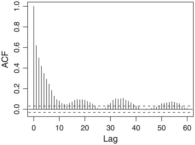
Figure 1 plots the autocorrelation function (ACF, Box and Jenkins 1976) of gene expression versus lag for the E. coli motility study. The microarray data (available at the NCBI web site with a series accession number GPL2101) were obtained in a direct pairwise comparison between a flhDC knock-out mutant and its isogenetic wild type strain. In this study, the ACF was calculated by considering gene expression levels on the E. coli chromosome as a one dimensional spatial series; and by convention, the lag in ACF was defined as the number of intervening genes plus one.

Figure 1.

The autocorrelation function of gene expression for the E. coli motility study. The ACF decays exponentially with the lag. It also shows a periodic pattern at larger lags.

Figure 1 shows strong expression correlation between gene neighbors along the linear chromosome. It decays exponentially with the lag. Such correlation has been studied and incorporated into microarray analysis to improve detection of differentially expressed genes by Xiao, Cavan, and Khodursky (2009).

Beyond the exponential decay, there are periodic patterns at larger lags. The nonmonotonic nature of the estimated ACF values may result from a higher-order organization of the chromosome, where the correlation pattern of expression of genes separated by certain large linear distances becomes similar to the pattern exhibited by linearly adjacent genes. As discussed in the Introduction, genes that are situated in spatial proximity are more likely to be coexpressed than distal genes. In order to link the coexpression of genes with their spatial proximity, the analysis must be extended from linear chromosome chains to 3D chromosome folding structures (Oliver and Misteli 2005). The periodic patterns in correlation, together with the periodic epi-organization of some genomes (Képès 2003, 2004), have motivated us to hypothesize helical chromosome structures, which can bring distant genes on a chromosomal DNA chain into close physical proximity. However, no formal mathematical model or a framework for statistical inference has been proposed to analyze helical chromosome structures in the literature. In subsequent sections, we describe a mathematical model for the helical structures, and demonstrate statistical and genomic evidence for such helical structures using gene expression data.

2.2 Mathematical Model

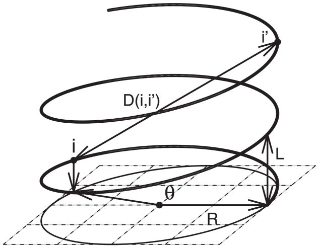
Figure 2 depicts a mathematical model of a helical chromosome structure. Suppose R is the radius of the structure, and L is the pitch. Then we can express the position of gene i in a Cartesian coordinate system as (x_i, y_i, z_i) = (R cos θ_i, R sin θ_i, Lθ_i/2π), where θ_i is the angle determined by the chromosome location of gene i. Note that a gene with angle θ + 2π is one loop higher than a gene with θ on the chromosome, although they are projected to the same point in the (x, y) plane. The 3D distance D_i,i′ between gene i and i′ is

Figure 2.

A mathematical model of the helical chromosome structure.

$$D_{i,i^{\prime }}\mid R,L={\left({(Rcos{\theta }_i-Rcos{\theta }_{i^{\prime }})}^2+{(Rsin{\theta }_i-Rsin{\theta }_{i^{\prime }})}^2+{\left(\frac{L{\theta }_i}{2\pi }-\frac{L{\theta }_{i^{\prime }}}{2\pi }\right)}^2\right)}^{1/2}.$$

Let d_i,i′ be the linear intergenetic distance (i.e., physical distance), between gene i and i′, which can be known for any gene pair in a well studied genome. Let θ_i,i′ ≡ θ_i′ − θ_i. Then θ_i,i′ = d_i,i′/R′, where $R^{\prime }\equiv \sqrt{R^2+{(\frac{L}{2\pi })}^2}$. For any given values of R and L, D_i,i′ is then determined by

$$D_{i,i^{\prime }}\mid d_{i,i^{\prime }},R,L=\sqrt{{\left(R-Rcos\frac{d_{i,i^{\prime }}}{R^{\prime }}\right)}^2+{\left(Rsin\frac{d_{i,i^{\prime }}}{R^{\prime }}\right)}^2+{\left(L\frac{d_{i,i^{\prime }}}{2\pi R^{\prime }}\right)}^2}.$$

2.3 Datasets

We use E. coli gene expression data (Sangurdekar, Srienc, and Khodursky 2006) and yeast cell cycle data (Spellman et al. 1998) as examples to explore the spatial correlation induced by 3D chromosome structures.

The E. coli set contains data from 217 cDNA microarray experiments carried out on E. coli K-12 strain MG1655, hybridized under different experimental conditions, which can be downloaded from the NCBI GeneOmnibus (series accession number GSE4357–GSE4380). It provides a comprehensive view about transcriptional responses of E. coli to various chemical, physiological, and genetic perturbations. On each array, the transcript abundance for each gene in an experimental sample was measured relative to a control and recorded as log2 ratio. The function annotations of E. coli genes were downloaded from the database EcoCyc (http://www.ecocyc.org) (Karp et al. 2002); and information about E. coli transcriptional regulation was downloaded from the RegulonDB database (Version 6.4, http://regulondb.ccg.unam.mx) (Gama-Castro et al. 2008).

In the yeast dataset, cDNA microarrays were used to study samples from a synchronized yeast culture, which reveal transcript levels of genes of the yeast Saccharomyces cerevisiae during a cell cycle. Fluorescence intensities from the red channel (experimental samples) and green channel (control samples) were measured and corrected for local background. The expression levels of more than 6000 open reading frames (ORFs) were determined as the log2 ratios of intensities between two channels. The dataset is publicly available (http://genome-www.stanford.edu/cellcycle) and contains expression data at different stages of a yeast cell cycle. Here, we used the data obtained in the cdc15-2 (DBY8728) yeast strain and the Saccharomyces Genome Database (http://www.yeastgenome.org) (Cherry et al. 1997) for information of gene location/sequence and functional annotations.

2.4 Exploratory Analysis

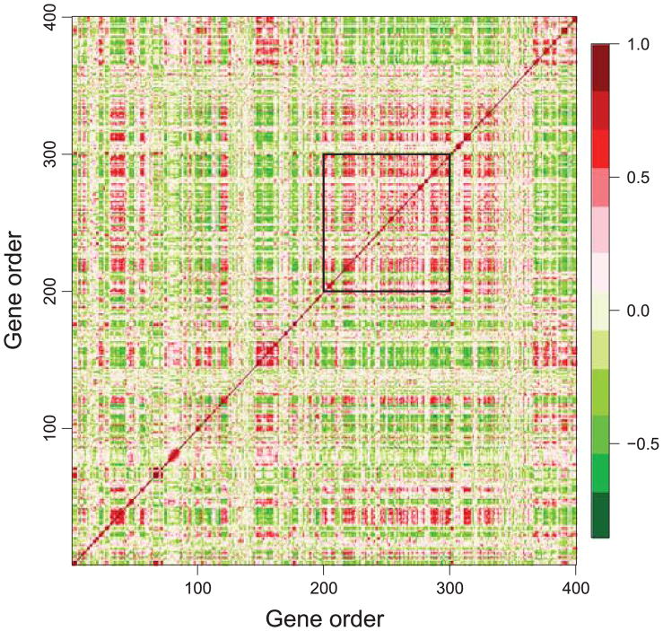
E. coli Data. Figure 3 shows a correlation map of the E. coli expression dataset, which plots the pairwise expression correlation between genes 1–400 by order on the chromosome. It shows coexpressed gene clusters along a linear chromosome. Further, it indicates that the genes that are far apart on a linear chromosome could be coexpressed, too. Notice that, the genes between 200 and 300, marked by the black rectangle, exhibit high correlation. Below we focus on this region and show statistical evidence that strongly supports the conjecture of helical folding structures.

Figure 3.

The correlation map of the E. coli expression dataset (genes 1–400). Genes 200–300 show high pairwise correlation, as marked in the black rectangle.

Unlike traditional spatial problems where distance matrices are known and spatial dependence can be explored by variograms or correlograms (Banerjee, Carlin, and Gelfand 2004), distance matrices here vary with the structural parameters R and L. Due to the lack of existing exploratory tools, we use an ad-hoc method to explore the association between the expression correlation and 3D distance as a function of (R, L), and demonstrate the strong association at some specific values of (R, L).

Let ρ_i,i′ be the Pearson correlation in gene expression and D_i,i′ be the 3D distance between gene i and i′. For any given values of R and L, we use a simple nonlinear regression model to aid our intuition,

$$\begin{array}{l}{\rho }_{i,i^{\prime }}=exp[-{\alpha }_0-{\alpha }_1{D}_{i,i^{\prime }}(R,L)]+{\epsilon }_{i,i^{\prime }},\\ {\epsilon }_{i,i^{\prime }}\sim \text{N}(0,{\sigma }^2).\end{array}$$ (1)

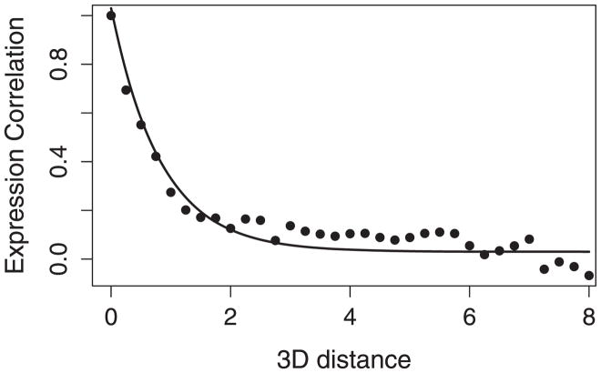
Here, we assume that the correlation between any gene pair decays exponentially with their physical distance. This is based on our empirical observation, as will be shown in Figure 6 below. Also, the above exponential model directly corresponds to AR1 models, which perform well in capturing the patterns of expression correlation along a linear chromosome (Xiao, Cavan, and Khodursky 2009). We also assume that ε_i,i′’s are iid for simplicity. In practice, ρ_i,i′’s are not independent. But (1) will help us to roughly explore the association between the correlation and 3D distance at different (R, L) values.

Figure 6.

The relationship between the expression correlation and 3D distance.

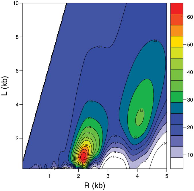
The contour plot of − log(p-value) for the chromosome segment B200–B300 of E. coli is given in Figure 4, for which p-values for testing α₁ = 0 were calculated from the nonlinear model based on different values of (R, L). There is strong evidence that, for certain values of R and L, the expression correlation of genes is associated with their 3D distance. For example, when R ≈ 2.0 and L ≈ 1.0, the − log(p-value) is more than 60. Also, we notice that there are two major peaks in the contour plot, which roughly correspond to (R, L) and (2R, 2L), respectively; and the highest peak occurs at (R, L). This is because if the helical structure with parameters R and L aligns a set of co-expressed genes altogether, then a larger helical structure with parameters mR and mL also partially aligns this set of genes into m groups, resulting in significant association. This concept is illustrated in Figure 5, where genes are represented by dots, with solid dots representing the coexpressed genes. Obviously, the multiple modes observed in the contour plot support the assumption of the helical structure very well.

Figure 4.

The contour plot of − log(p-value) at different values of R and L for the E. coli expression dataset (genes 200–300).

Figure 5.

The helical structures with parameters (R, L) and (2R, 2L). The solid dots represent a set of genes that are aligned into 3D proximity by the helical structures.

Figure 6 shows the approximate relationship between the expression correlation and 3D distance, calculated by fixing R = 2 and L = 1 (corresponding to the highest peak in Figure 4). The dots represent the averaged values of expression correlation at different 3D distances, and the solid curve represents the fitted exponential decay model. The model seems to work reasonably well.

Yeast Data

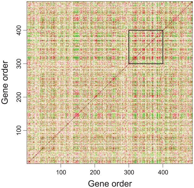
Figure 7 shows the correlation map of the yeast cell cycle dataset for all the genes on chromosome 16. The black rectangle (300–400) shows several clusters of coexpressed genes along the linear chromosome. These clusters are roughly evenly spaced on the chromosome, showing high pairwise expression correlation. In addition, as reported by Képès (2003, 2004), the transcriptional binding sites of some key regulators are evenly spaced on the yeast chromosome. All these support the hypothesis that the chromosome forms helical structures, which may facilitate coexpression of otherwise distal genes.

Figure 7.

The correlation map of the Yeast Cell Cycle dataset (genes 1–486 on chromosome 16). Genes 300–400 show high pairwise correlation, as marked in the black rectangle.

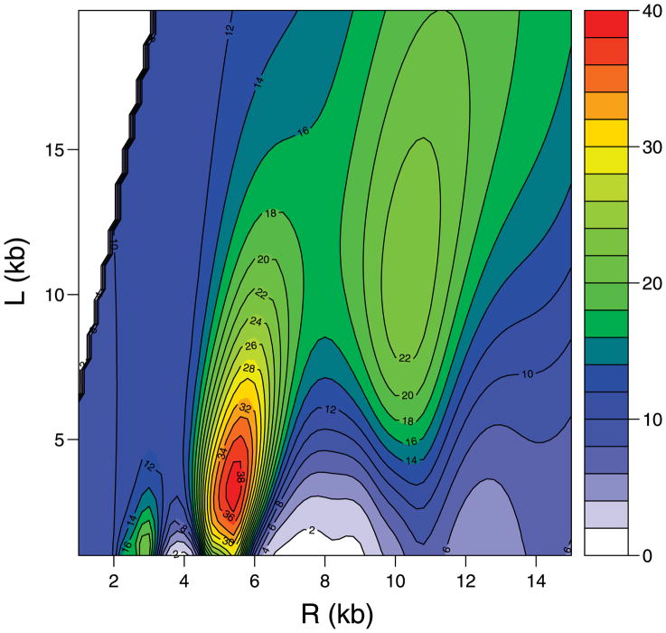
Figure 8 shows the corresponding contour plot of − log(p-value). We can see that the p-value is most significant when R = 5.2 and L = 2.5, with − log(p-value) around 40. There are other local peaks roughly corresponding to (R/2, L/2) and (2R, 2L). Again, this can be explained well by that the helical structures with parameters nR/m and nL/m partially align genes, resulting in significant association.

Figure 8.

The contour plot of − log(p-value) at different values of R and L for the yeast cell cycle dataset (genes 300–400 on chromosome 16).

3. STATISTICAL MODEL AND INFERENCE

Let Y_ij be the gene expression (log ratio of test sample versus control sample) of gene i on microarray j, i = 1, …, G and j = 1, …, n, where G is the total number of genes and n is the number of microarrays. Let μ_ij be the mean expression level of gene i in microarray j, and ${\sigma }_i^2$ be the variance for gene i. We assume that for i = 1, …, G and j = 1, …, n,

$$Y_{ij}={\mu }_{ij}+{\epsilon }_{ij},{\epsilon }_{ij}\stackrel{\text{iid}}{\sim }\text{N}(0,{\sigma }_i^2),$$ (2)

where μ_ij is the true expression level of gene i on array j; and ε_ij’s are measurement errors that are assumed to be independent across all genes and arrays. Because of the coexpression of the spatially proximate genes, the mean vector for array j, ${({\mu }_{ij})}_{i=1}^G$, is modeled by N(0, Σ), where the covariance matrix Σ is specified by

$${\mathrm{\sum }}_{i,i^{\prime }}={\tau }^2{e}^{-\beta D_{i,i^{\prime }}(R,L)}.$$ (3)

From (3), we can see that Var(μ_ij) = τ², and Corr(μ_ij, μ_{i′ j}) = e^{−βD_i,i′(R,L)} that is modeled by an exponential function of the distance D_i,i′. This is consistent with the empirical evidence that the correlation decays exponentially as the distance of genes becomes larger. Also, Σ is guaranteed to be a symmetric and positive definite matrix, since the exponential of a symmetric matrix is a symmetric positive-definite matrix (Moakher and Batchelor 2006).

Define ${\mathbf{Y}}_j={(Y_{ij})}_{i=1}^G$, the vector of observed expression levels from array j, and Y = (Y₁, …, Y_n), the G × n matrix of all data. Let μ = (μ₁, …, μ_n) be the G × n matrix of all mean levels, and the diagonal matrix $\mathbf{C}=\text{diag}({\sigma }_1^2,\dots ,{\sigma }_G^2)$. Then the proposed model can be rewritten as

$$\begin{array}{l}{\mathbf{Y}}_j\mid {\mathit{\mu }}_j,\mathbf{C}\sim \text{N}({\mathit{\mu }}_j,\mathbf{C}),\\ {\mathit{\mu }}_j\mid {\tau }^2,\beta ,R,L\sim \text{N}(\mathbf{0},\mathbf{\sum }).\end{array}$$

The full probability model is given by

$$\begin{array}{l}p(\mathbf{Y},\mathrm{\Theta })=p(\mathbf{Y}\mid \mathit{\mu },\mathbf{C})p(\mathit{\mu }\mid {\tau }^2,\beta ,R,L)\pi (\mathbf{C},{\tau }^2,\beta ,R,L)\\ =\prod _{j=1}^n\{\text{N}({\mathbf{Y}}_j\mid {\mathit{\mu }}_j,\mathbf{C})\text{N}({\mathit{\mu }}_j\mid \mathbf{0},\mathbf{\sum })\}\times \prod _{i=1}^G\pi ({\sigma }_i^2)·\pi ({\tau }^2)·\pi (\beta )\pi (R)\pi (L),\end{array}$$

where Θ is the collection of all involved (hyper)parameters in the model, π’s are prior distributions, and ${\sigma }_i^2$’s, τ², β, R, and L are all assumed to be a priori independent. For all the variance components, we specify conjugate inverse gamma priors, that is, ${\sigma }_i^2\sim \text{IG}({\alpha }_{\sigma },{\gamma }_{\sigma })$ for i = 1, …, G, and τ² ~ IG(α_τ, γ_τ), where the hyperparameters are chosen to make the prior very vague, for example, IG(0.01, 0.01). We specify uniform priors for R and L, that is π (R) π (L) ∝ 1 with 0 < R < R_max and 0 < L < L_max. The upper bounds R_max and L_max can be both chosen as the diameter of the relevant cell, which the chromosome under consideration must be fit in. We consider a truncated normal prior for β (say mean β₀, variance ${\sigma }_{\beta }^2$) truncated at zero. The variance ${\sigma }_{\beta }^2$ is chosen to be sufficiently large so that the prior is weak (i.e., nearly flat) and the location of its mean is irrelevant. Then the posterior distribution is

$$\begin{array}{l}p(\mathrm{\Theta }\mid \mathbf{Y})\propto p(\mathbf{Y},\mathrm{\Theta })\\ \propto \prod _{j=1}^n\left\{{\mid \mathbf{C}\mid }^{-1/2}exp\left[-\frac{1}{2}{({\mathbf{Y}}_j-{\mathit{\mu }}_j)}^T{\mathbf{C}}^{-1}({\mathbf{Y}}_j-{\mathit{\mu }}_j)\right]\right\}\\ ·\prod _{j=1}^n{\mid \mathbf{\sum }\mid }^{-1/2}exp\left(-\frac{1}{2}{\mathit{\mu }}_j^T{\mathbf{\sum }}^{-1}{\mathit{\mu }}_j\right)\\ ·exp\left[-\frac{{(\beta -{\beta }_0)}^2}{2{\sigma }_{\beta }^2}\right]·I(\beta >0)\\ ·\prod _{i=1}^G\left[{\left(\frac{1}{{\sigma }_i^2}\right)}^{{\alpha }_{\sigma }+1}exp\left(-\frac{{\gamma }_{\sigma }}{{\sigma }_i^2}\right)\right]\\ ·{\left(\frac{1}{{\tau }^2}\right)}^{{\alpha }_{\tau }+1}exp\left(-\frac{{\gamma }_{\tau }}{{\tau }^2}\right),\end{array}$$

where I(·) is an indicator function.

Now we can derive the full conditional posterior distributions. We use Θ\θ to denote the collection of all the parameters in Θ except for θ.

For j = 1, …, n,

$${\mathit{\mu }}_j\mid \mathbf{Y},\mathrm{\Theta }\backslash {\mathit{\mu }}_j\sim \text{N}[{\mathbf{C}}^{-1}{({\mathbf{C}}^{-1}+{\mathbf{\sum }}^{-1})}^{-1}{\mathbf{Y}}_j,{({\mathbf{C}}^{-1}+{\mathbf{\sum }}^{-1})}^{-1}].$$ (4)

For the variance of measurement errors ${\sigma }_i^2$,

$${\sigma }_i^2\mid \mathbf{Y},\mathrm{\Theta }\backslash {\sigma }_i^2\sim \text{IG}\left({\alpha }_{\sigma }+\frac{n}{2},{\gamma }_{\sigma }+\frac{1}{2}\sum _{j=1}^n{(Y_{ij}-{\mu }_{ij})}^2\right).$$

For the variance τ² of μ_ij’s,

$$\begin{array}{l}{\tau }^2\mid \mathbf{Y},\mathrm{\Theta }\backslash {\tau }^2\sim \text{IG}\left({\alpha }_{\tau }+\frac{G}{2},{\gamma }_{\tau }+\frac{1}{2}\sum _{j=1}^n{\mathit{\mu }}_j^T{\mathbf{\Xi }}^{-1}{\mathit{\mu }}_j\right).\\ \mathbf{\Xi }={(e^{-\beta D_{i,i^{\prime }}(R,L)})}_{G\times G}.\end{array}$$

For the parameters β, R, and L,

$$\begin{array}{l}p(\beta ,R,L,\mid \mathbf{Y},\mathrm{\Theta }\backslash \{\beta ,R,L\})\propto \prod _{j=1}^n{\mid \mathbf{\sum }\mid }^{-1/2}exp\left(-\frac{1}{2}{\mathit{\mu }}_j^T{\mathbf{\sum }}^{-1}{\mathit{\mu }}_j\right)·exp\left[-\frac{{(\beta -{\beta }_0)}^2}{2{\sigma }_{\beta }^2}\right]·I(\beta >0).\end{array}$$

We are primarily interested in inferring the structural parameters R and L, and β which quantifies the association between expression correlation of genes and their 3D distance. We use a Gibbs sampler to obtain the posterior draws of the parameters. According to the full conditionals, the parameters μ_j, ${\sigma }_i^2$, τ² can be sampled directly, while β, R, and L can be sampled using a built-in M-H algorithm. For each dataset, we run 20,000 iterations and use 50% for burn-in. Numerical experience indicates that the posterior distribution for R and L may be complex and have multiple modes. To facilitate the convergence of the MCMC chains, we use the parameters estimated from the exploratory analysis to set the initial values for the algorithm. We get rough estimates of R and L from where the − log₁₀(p-value) is maximized, and that of β through the relationship β = α₁. Standard techniques (Brooks and Roberts 1998) are used to assess the sensitivity and validity of the model.

Alternatively, we may consider the maximum likelihood method for parameter estimation. To simplify the computation, we treat σ_i’s as nuisance parameters, and estimate σ_i using the sample standard deviation of expression levels of gene i. We can integrate out each μ_j to obtain the marginal distribution of Y|R, L, β, τ²,

$$p(\mathbf{Y}\mid R,L,\beta ,{\tau }^2)=\prod _{j=1}^n\frac{1}{{\mid \mathbf{C}+\mathbf{\sum }\mid }^{1/2}}exp\left[-\frac{1}{2}{\mathbf{Y}}_j^T{(\mathbf{C}+\mathbf{\sum })}^{-1}{\mathbf{Y}}_j\right].$$

The MLE (maximum likelihood estimator) of (R, L, β, τ²) is

$$(\widehat{R},\widehat{L},\widehat{\beta },{\widehat{\tau }}^2)=\text{argmax}[p(\mathbf{Y}\mid R,L,\beta ,{\tau }^2)],$$

which can be estimated using a quasi-Newton method (i.e., the variable metric algorithm; see Byrd et al. 1995). Again, we use the parameters estimated from the exploratory analysis to set the initial values for the algorithm. Plugging in the MLE and the sample standard deviation for σ_i’s, we can get spatially smoothed estimates of μ_ij’s based on (4).

In our numerical experiments, we find that the results from the fully Bayesian approach are very similar to those from the MLE approach. In this paper, we present the results based on the fully Bayesian approach for consistency, while the MLE approach could be used as an efficient method for estimation.

4. SIMULATION

Suppose R₀ and L₀ are the true radius and the pitch for a chromosome structure, respectively. From the exploratory analysis, we have noticed that the correlation in gene expression levels is strongly associated with the 3D distance, when the parameters R and L equal mR₀ and mL₀. This could cause the proposed model to have a complex likelihood surface with multiple modes. Before we applied the proposed model to real data, we conducted simulation to explore the characteristics of the likelihood surface and also examined the performance of estimation using the proposed Bayesian approach.

In the first simulation, we set R₀ = 2, L₀ = 1, β = 0.1, τ² = 0.4², ${\sigma }_i^2={0.5}^2$, n = 200, and G = 100. The mean expression levels for microarray j were simulated from μ_j|Σ ~ N(0, Σ) with the covariance matrix Σ = 0.4²[e^{−0.1D_i,i′(2,1)}] and the observed gene expression levels were simulated from Y_ij|μ_ij, ${\sigma }_i^2\sim \text{N}({\mu }_{ij},{0.5}^2)$.

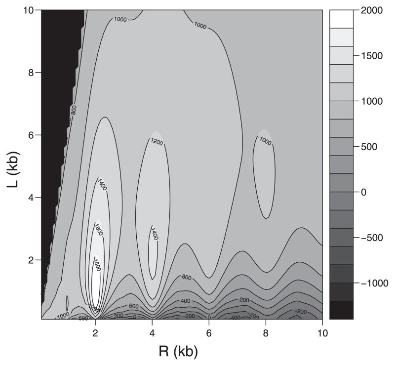
We first explored the dependence of the likelihood on R and L. With μ_j’s integrated out, the marginal likelihood only depends on the values of R and L after we plug in the true values of β, τ, and ${({\sigma }_i)}_{i=1}^n$. Figure 9 displays the contour plot of log for different values of R and L, which clearly confirms our conjecture that the likelihood function has multiple modes due to the helical structure of the chromosome. Besides the mode corresponding to R = R₀ and L = L₀, we can see from the plot that there are other modes at (mR₀, mL₀). We also noticed that the value of log at (R₀, L₀) is much higher (more than 200) than those of the other modes, indicating that although the log likelihood surface is multimodal, the true solution is very distinct from the other modes and can be easily identified.

Figure 9.

The profile log-likelihood (up to a normalizing constant) surface for different values of R and L in Simulation 1.

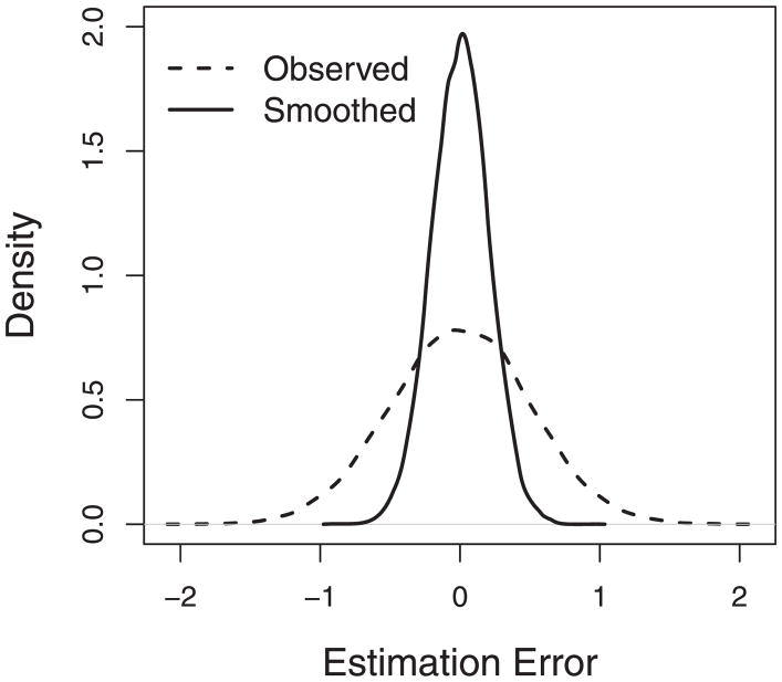
Under helical structures, our approach is expected to perform well in estimation of expression levels. To confirm this, we report the densities of the estimation errors for the smoothed expression μ̂_ij and the observed expression Y_ij in Figure 10. Here, μ̂_ij, the posterior mean of μ_ij, is a smoothed estimator that can borrow strength from the spatially correlated genes, while the observed value of Y_ij is a natural estimator of the gene expression level. We define the estimation error of μ̂_ij to be the difference between μ̂_ij and the true value μ_ij, and compare that to the error of the natural estimator Y_ij. It is clear that in general, μ̂_ij has a smaller estimation error than Y_ij. The mean squared error (MSE) for μ̂_ij is 0.04, while that for Y_ij is 0.25. The results show that the smoothed expression μ̂_ij performs better than the observed expression Y_ij in estimating μ_ij.

Figure 10.

The density plot of estimation errors in Simulation 1. The dashed line is for the observed expression Y_ij, and the solid line for the smoothed expression μ̂_ij.

We conducted several simulation studies to check under helical structures, whether the proposed model could lead to reasonable estimation of parameters and gene expression as expected. The posterior estimates of parameters, as well as the MSEs for the estimators of expression levels, are summarized in Table 1. In all the simulation studies, parameters were estimated very well and again, μ̂_ij did better than Y_ij. The results also indicate that the MSE from the proposed model decreases as β decreases. It is because when β decreases, the correlation between two genes decreases more slowly with their 3D distance so that overall, the correlation values get higher. In this case, incorporating the chromosomal spatial correlation into the analysis can greatly reduce estimation errors. Further, for larger τ², the noise in the correlation is larger, and so the estimation errors of the proposed model increase.

Table 1.

Results from simulation studies

	Simulation settings				Parameter estimation				MSE
	R	L	β	τ2	R	L	β	τ2	Yij	μ̂ij
S1	2.0	1.0	0.1	0.16	2.01 ± 0.01	1.04 ± 0.07	0.10 ± 0.01	0.16 ± 0.01	0.25	0.04
S2	2.0	1.0	0.2	0.16	2.01 ± 0.01	0.98 ± 0.05	0.20 ± 0.02	0.16 ± 0.01	0.25	0.07
S3	2.0	1.0	0.3	0.16	2.00 ± 0.01	1.04 ± 0.06	0.29 ± 0.02	0.16 ± 0.01	0.25	0.08
S4	2.0	1.0	0.4	0.16	2.00 ± 0.01	1.03 ± 0.06	0.38 ± 0.02	0.16 ± 0.01	0.25	0.10
S5	2.0	1.0	0.1	0.64	2.01 ± 0.01	1.03 ± 0.04	0.10 ± 0.01	0.65 ± 0.04	0.25	0.08
S6	2.0	1.0	0.2	0.64	2.01 ± 0.01	1.02 ± 0.04	0.19 ± 0.01	0.67 ± 0.03	0.25	0.12
S7	2.0	1.0	0.3	0.64	2.00 ± 0.01	0.99 ± 0.03	0.29 ± 0.01	0.64 ± 0.02	0.25	0.15
S8	2.0	1.0	0.4	0.64	2.01 ± 0.01	1.06 ± 0.06	0.39 ± 0.01	0.65 ± 0.0	0.25	0.18

5. APPLICATIONS

We applied the proposed model to gene expression profiles in different regions of the E. coli and yeast chromosomes using datasets described in Section 2.3. Our goal was to infer the radius R and the pitch L to characterize the chromosome structure for each of these regions.

As will be discussed in Section 6, chromosome folding structures can be very complex, and regions where different helical structures may form are unknown. Since there is no existing method to detect such regions, we used a simple method to narrow down the chromosome regions with possible helical structures. That is, a whole chromosome is scanned by first dividing it into some smaller windows (to show necessary detail); for each window, we draw the correlation plot of chromosome expression and then find regions that show high correlations (e.g., the black box in Figure 3). Second, we apply our exploratory analysis described in Section 2.4 to the regions to examine whether there exists strong evidence for helical structures. Below we report results from several example regions identified by the outlined method.

5.1 E. coli Data

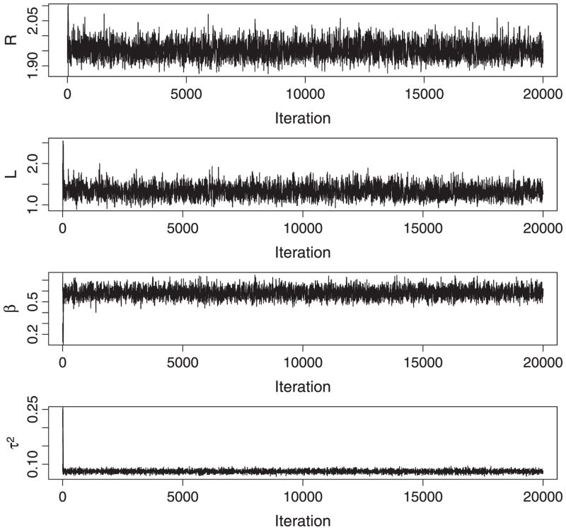
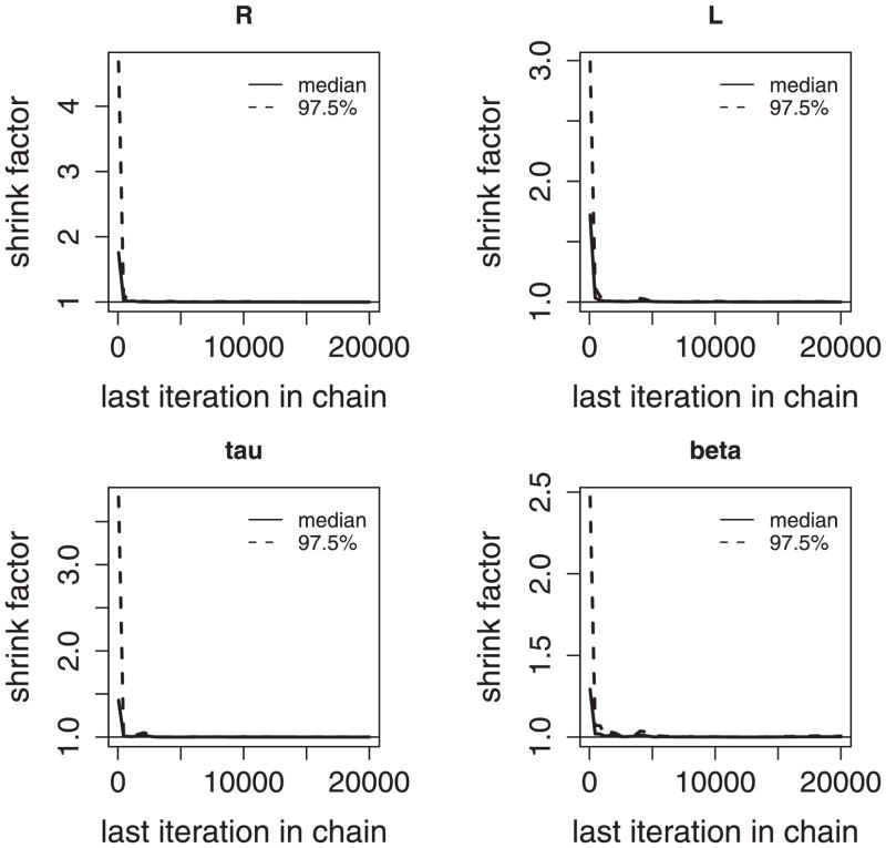
We first applied the proposed model to the gene expression profiles in the region B200–B300 of the E. coli chromosome. From the exploratory analysis (Figure 4), we estimated the initial values R = 2.0, L = 1.0, β = 0.39, and τ² = 1.40. We used the MCMC simulation to draw samples from the posterior distribution. For each parameter, the trace plot of MCMC iterations with three chains is given in Figure 11; and the plot of the median potential scale reduction factor along with its 97.5% quantile (Gelman and Rubin 1992) is given in Figure 12. From the trace plots, we can see that the posterior draws are well mixed and there is no clear trend in the sample space of the parameters. The Gelman and Rubin diagnostics show that all the shrink factors converge to 1. All these indicate the convergence of the chains.

Figure 11.

Trace plots of MCMC iterations in the region B200–B300 of the E. coli chromosome. The three chains are mixed well for all the parameters.

Figure 12.

Plots of the potential scale reduction factor in the region B200–B300 of the E. coli chromosome.

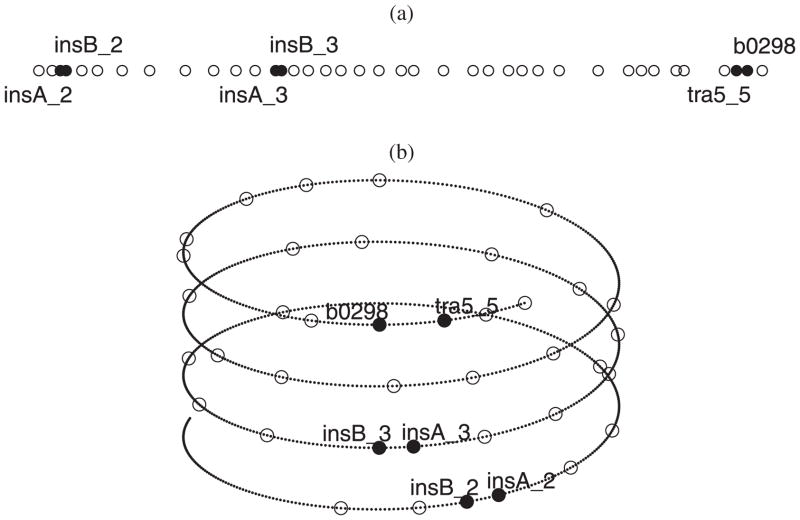
Figure 13(a) shows the chromosome region as a linear chromosome chain. The solid dots represent the genes that belong to the “extrachromosomal transposon related” function group (the EcoCyc database, http://www.ecocyc.org), and the circles represent other genes in this region. Using the posterior mean of R (2.0) and L (1.3), we reconstructed the helical chromosome folding structure, shown in Figure 13(b). We notice that, by forming the helical structure, genes insA-2, insB-2, insA-3, insB-3, B0298, and tra5-5 are brought into spatial proximity. The 3D distances among these genes are less than 6 kbs, while in the linear structure [Figure 13(a)], the distance from insA-2 to B0298 is about 50 kbs. The genes insA-2, insB-2, insA-3, and insB-3 together are the coding genes for IS1 proteins (InsA and InsB); B0298 (insE) and tra5-5 (insF) are the coding genes for IS3 element proteins. All of these proteins are involved in mobilization of insertion sequences which encode these proteins. The proposed spatial clustering of insertion elements is intriguing. First, despite belonging to two different families, genes in the insertion cassettes are likely to be coregulated, insuring family-independent coordinated responses to conditions which may trigger transposition events. Such a strategy would allow for a more efficient proliferation of mobile elements than the one based on a family-specific mobilization. Second, very little is known about how the distribution of transposons and insertion elements across a genome is controlled. The current analysis offers the possibility that acceptor sequences are not randomly distributed along the bacterial chromosome and that the chromosomal hyper-structure may underlie such distribution.

Figure 13.

The chromosome structure for the region B200–B300 of the E. coli chromosome: (a) the linear chromosome chain; (b) the helical chromosome folding structure (enlarged 10 times to show the detail).

We also applied the proposed model to the regions B2700–B2800 and B3400–B3500 of the E. coli chromosome. Convergence was detected by checking trace plots and plots of the potential scale reduction factor for all the parameters (figures omitted due to the space limit).

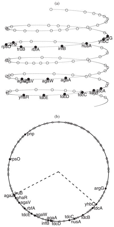
The helical chromosome structure for the region B3100–B3200, reconstructed using the posterior means R̂= 2.7 and L̂= 5.3, is shown in Figure 14(a), where solid dots represent genes regulated by CRP (i.e., the cAMP Receptor Protein), and circles represent the other genes. In this region, CRP binds to 18 genes: tdcE, tdcD, tdcC, tdcB, tdcA, kbaZ, agaV, agaW, agaA, pnp, rpsO, truB, rbfA, infB, nusA, rimP, metY, and argG (the RegulonDB database, Version 6.4, http://regulondb.ccg.unam.mx; Gama-Castro et al. 2008). These genes are far apart on the linear chromosome chain. However, according to our results, the helical structure would place 15 out of the 18 CRP regulated genes into a relative proximity that corresponds to the dashed sector (about 120°) in Figure 14(b). In contrast, the density of the genes is much less in the remaining part of the chromosome. Note that the density ratio is roughly 15/1 vs. 3/2, that is, 10 versus 1. This strongly support the notion that by forming a helical structure, the CRP regulated genes are rearranged into a close 3D spatial proximity, which could greatly facilitate the coregulation of these genes.

Figure 14.

The chromosome structure for the region B3100–B3200 of the E. coli chromosome: (a) the helical chromosome folding structure; (b) a top view of the helical structure to show the alignment of genes. It shows that 15 out of the 18 CRP regulated genes are placed into a relative proximity that corresponds to the dashed sector (about 120°).

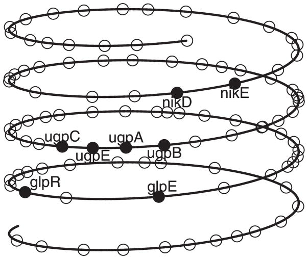
The helical chromosome structure for the region B3400–B3500, reconstructed using the posterior means R̂ = 4.3 and L̂ = 5.7, is shown in Figure 15. In this region, there are eight genes (glpR, glpE, ugpC, ugpE, ugpA, ugpB, nikD, and nikE) that belong to the anaerobic respiration functional group (the EcoCyc database). These genes are arranged very close to each other by the folding structure. Anaerobic respiration is an important way for E. coli to produce usable energy without oxygen, and the spatial proximity could help these genes coordinate their expression to carry out the biological function.

Figure 15.

The chromosome structure for the region B3400–B3500 of the E. coli chromosome.

For the three regions above, the circumferences of the helices are found to be about 12–28 kbs. This result agrees with the recent observation reported by biological studies (e.g., Postow et al. 2004; Carpentier et al. 2005) that E. coli genes are organized into topological domains with size on the order 10 kbs, where helical hyper-structures can be viewed as a means of axial packing of the supercoiled loops.

5.2 Yeast Data

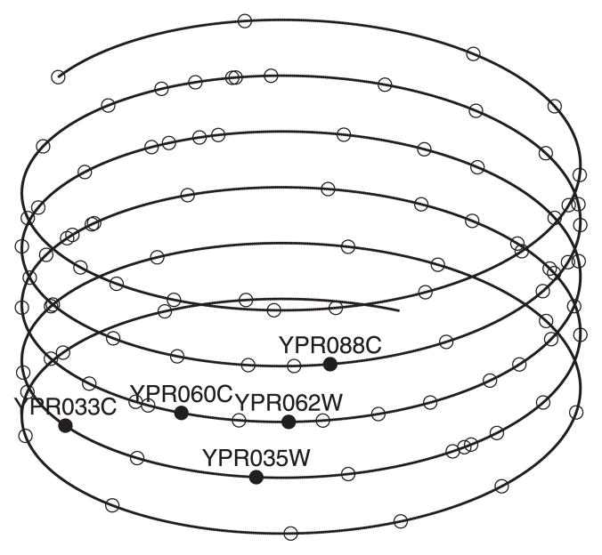
We applied the proposed model to the region 300–400 of the yeast chromosome. Again, the convergence was detected from trace plots and Gelman and Rubin diagnostics. The helical chromosome structure, reconstructed using the posterior means R̂ = 5.4 and L̂ = 2.3, is shown in Figure 16. The solid dots represent the five genes, YPR033C, YPR035W, YPR060C, YPR062W, and YPR088C, which belong to the cytoplasm function group (GO: 0005737). They are highly coexpressed, whose pairwise expression correlations range from 0.73 to 0.94 with mean 0.83. The figure shows that through the chromosome folding structure, the genes that are distant on the linear chromosome are now sufficiently close, especially for the three genes YPR035W, YPR060C, and YPR088C.

Figure 16.

The chromosome structure for the region 300–400 of the yeast chromosome.

6. DISCUSSION

Biological studies have shown that chromosomes are highly organized and the spatial arrangement plays an important role in gene regulation. From a functional point of view, it is more efficient for living organisms to utilize chromosome folding to facilitate coordinated regulation of gene expression. Understanding 3D chromosome structures will greatly advance our understanding of how genes and proteins work together to maintain life. In this paper, we have presented sound evidence that spatial patterns of gene expression can be explained by helical chromosome folding structures. We have demonstrated that there exists a strong association between the expression correlation of genes and their distance in 3D space. We have proposed a Bayesian hierarchical method based on helical structures to incorporate the spatial correlation into microarray analysis and to infer the structural parameters.

Through real data examples, we have shown that the proposed model reveals an intriguing biological phenomenon: a group of genes can be brought into spatial proximity which in turn may greatly facilitate coordination in regulation of their transcription. This brings about a new understanding of gene regulation. From a functional prospective, structural organization of the chromosome may contribute to a more orderly processing and utilization of genetic information on a genome-wide scale. For example, spatial colocalization of regulatory sequences recognized by one transcription factor may result in substantial reduction of space which needs to be searched by the regulator before steady-state binding to cognate sequences is achieved. Consistent with that was an observation made by Képès (2003) that members of many regulons (a regulon is defined as a set of genes controlled by one regulator) in both E. coli and Saccharomyces are distributed along linear chromosomal dimensions with certain significant periodicity. Such periodic patterns can be most naturally accommodated within an underlying spiral organization of the chromosome, whose existence we argue in the current study from a statistical prospective.

Furthermore, our predictions of the loop sizes, which correspond to the circumference of the helical cross-section in our geometric model, agree with the estimates of supercoiled domain sizes obtained from the analysis of intergenetic distances (Carpentier et al. 2005) and spectral analysis of gene expression patterns (Jeong, Ahn, and Khodursky 2004). Thus, using different approaches, these studies, including ours, revealed similar features of chromosomal organization, which likely form the basis of DNA packing in living chromosomes.

There is no indication that chromosome folding structures should be conserved across organisms or even within the same organism, the parameters of folding structures or even structures themselves are different in different regions of the same chromosome, and they may change in response to different environmental conditions and across samples. Thus, in our analysis of experimental data, we applied the proposed model to selected chromosomal regions instead of entire chromosomes. According to our exploratory analysis, those regions exhibited statistically significant spatial correlations which in turn can be interpreted in terms of underlying structural organization of the DNA template. It does not imply, however, that other chromosomal regions, not included in the study, have to be structurally disorganized. We hypothesized that actively transcribed genes, in a nucleoid or in a chromosome, may be organized in a spatial structure, for example, helix, that facilitates readout of genetic information within a certain time frame, in a certain condition. However, to make the problem tractable, we had to assume a shared structure across different conditions and samples. In the future, it would be very interesting to study how the structures are dynamically formed at different chromosome regions in response to different environmental stimulations (experimental conditions) across samples. For example, a more flexible helical structure (i.e., helices with varying parameters at different locations) might be considered as a first extension of the mathematical model for 3D chromosome structures. Finally, in this study, we only focused on chromosome structures at a medium range (10–100 kbs), while regional structures are likely to form some even higher order structure at a longer range (~1000 kbs). All these extensions could be topics for future studies to better understand the 3D chromosome structures at different levels and their roles in carrying out biological functions.

In summary, this article presents the first and successful attempt at statistical modeling of complex gene expression patterns within an explicit geometric framework of chromosomal organization. Our study leads to interesting biological insights and introduces the method of hierarchical modeling into a new area of applications.

References

- Aggarwal A, Leong SH, Lee C, Kon OL, Tan P. Wavelet Transformations of Tumor Expression Profiles Reveals a Pervasive Genome-Wide Imprinting of Aneuploidy on the Cancer Transcriptome. Cancer Research. 2005;65(1):186–194. [PubMed] [Google Scholar]
- Banerjee S, Gelfand AE. Bayesian Wombling. Journal of the American Statistical Association. 2006;101(476):1487–1501. doi: 10.1198/016214506000000041. [DOI] [PMC free article] [PubMed] [Google Scholar]
- Banerjee S, Carlin BP, Gelfand AE. Hierarchical Modeling and Analysis for Spatial Data. New York: Chapman & Hall; 2004. [Google Scholar]
- Boutanaev AM, Kalmykova AI, Shevelyov YY, Nurminsky DI. Large Clusters of Co-Expressed Genes in the Drosophila Genome. Nature. 2002;420(6916):666–669. doi: 10.1038/nature01216. [DOI] [PubMed] [Google Scholar]
- Box G, Jenkins G. Time Series Analysis: Forecasting and Control. Oakland: Holden-Day; 1976. revised. [Google Scholar]
- Brooks S, Roberts G. Convergence Assessment Techniques for Markov Chain Monte Carlo. Statistics and Computing. 1998;8:319–335. [Google Scholar]
- Byrd R, Lu P, Nocedal J, Zhu C. A Limited Memory Algorithm for Bound Constrained Optimization. SIAM Journal on Scientific Computing. 1995;16:1190–1208. [Google Scholar]
- Caron H, van Schaik B, van der Mee M, Baas F, Riggins G, van Sluis P, Hermus MC, van Asperen R, Boon K, Voute PA, Heisterkamp S, van Kampen A, Versteeg R. The Human Transcriptome Map: Clustering of Highly Expressed Genes in Chromosomal Domains. Science. 2001;291(5507):1289–1292. doi: 10.1126/science.1056794. [DOI] [PubMed] [Google Scholar]
- Carpentier A-S, Torresani B, Grossmann A, Henaut A. Decoding the Nucleoid Organisation of Bacillus subtilis and Escherichia coli Through Gene Expression Data. BMC Genomics. 2005;6(1):84. doi: 10.1186/1471-2164-6-84. [DOI] [PMC free article] [PubMed] [Google Scholar]
- Cherry J, Ball C, Weng S, Juvik G, Schmidt R, Adler C, Dunn B, Dwight S, Riles L, Mortimer RK, Botstein D. Genetic and Physical Maps of Saccharomyces cerevisiae. Nature. 1997;387:67–73. [PMC free article] [PubMed] [Google Scholar]
- Cohen BA, Mitra RD, Hughes JD, Church GM. A Computational Analysis of Whole-Genome Expression Data Reveals Chromosomal Domains of Gene Expression. Nature Genetics. 2000;26(2):183–186. doi: 10.1038/79896. [DOI] [PubMed] [Google Scholar]
- Cooper S. Human Gene Evolution. San Diego, CA: Academic Press; 1999. [Google Scholar]
- Eichler EE, Sankoff D. Structural Dynamics of Eukaryotic Chromosome Evolution. Science. 2003;301(5634):793–797. doi: 10.1126/science.1086132. [DOI] [PubMed] [Google Scholar]
- Gama-Castro S, Jimenez-Jacinto V, Peralta-Gil M, Santos-Zavaleta A, Penaloza-Spinola MI, Contreras-Moreira B, Segura-Salazar J, Muniz-Rascado L, Martinez-Flores I, Salgado H, Bonavides-Martinez C, Abreu-Goodger C, Rodriguez-Penagos C, Miranda-Rios J, Morett E, Merino E, Huerta AM, Trevino-Quintanilla L, Collado-Vides J. RegulonDB (Version 6.0): Gene Regulation Model of Escherichia coli K-12 Beyond Transcription, Active (Experimental) Annotated Promoters and Textpresso Navigation. Nucleic Acids Research. 2008;36(Suppl 1):D120–124. doi: 10.1093/nar/gkm994. [DOI] [PMC free article] [PubMed] [Google Scholar]
- Gelman A, Rubin DB. Inference From Iterative Simulation Using Multiple Sequences. Statistical Science. 1992;7:457–511. [Google Scholar]
- Hanin L, Awadalla SS, Cox P, Glazko G, Yakovlev A. Chromosome-Specific Spatial Periodicities in Gene Expression Revealed by Spectral Analysis. Journal of Theoretical Biology. 2009;256:333–342. doi: 10.1016/j.jtbi.2008.10.015. [DOI] [PubMed] [Google Scholar]
- Hurst LD, Pal C, Lercher MJ. The Evolutionary Dynamics of Eukaryotic Gene Order. Natute Reviews Genetics. 2004;5(4):299–310. doi: 10.1038/nrg1319. [DOI] [PubMed] [Google Scholar]
- Jeong KS, Ahn J, Khodursky AB. Spatial Patterns of Transcriptional Activity in the Chromosome of Escherichia coli. Genome Biology. 2004;5:R86. doi: 10.1186/gb-2004-5-11-r86. [DOI] [PMC free article] [PubMed] [Google Scholar]
- Karp PD, Riley M, Saier M, Paulsen IT, Collado-Vides J, Paley SM, Pellegrini-Toole A, Bonavides C, Gama-Castro S. The Eco-Cyc Database. Nucleic Acids Research. 2002;30(1):56–58. doi: 10.1093/nar/30.1.56. [DOI] [PMC free article] [PubMed] [Google Scholar]
- Képès F. Periodic Epi-Organization of the Yeast Genome Revealed by the Distribution of Promoter Sites. Journal of Molecular Biology. 2003;329(5):859–865. doi: 10.1016/s0022-2836(03)00535-7. [DOI] [PubMed] [Google Scholar]
- Képès F. Periodic Transcriptional Organization of the E. coli Genome. Journal of Molecular Biology. 2004;340(5):957–964. doi: 10.1016/j.jmb.2004.05.039. [DOI] [PubMed] [Google Scholar]
- Khorasanizadeh S. The Nucleosome: From Genomic Organization to Genomic Regulation. Cell. 2004;116(2):259–272. doi: 10.1016/s0092-8674(04)00044-3. [DOI] [PubMed] [Google Scholar]
- Kruglyak S, Tang H. Regulation of Adjacent Yeast Genes. Trends in Genetics. 2000;16(3):109–111. doi: 10.1016/s0168-9525(99)01941-1. [DOI] [PubMed] [Google Scholar]
- Li Q, Lee BTK, Zhang L. Genome-Scale Analysis of Positional Clustering of Mouse Testis-Specific Genes. BMC Genomics. 2005;6(1):7. doi: 10.1186/1471-2164-6-7. [DOI] [PMC free article] [PubMed] [Google Scholar]
- Liang S, Banerjee S, Carlin BP. Bayesian Wombling for Spatial Point Processes. Biometrics. 2009;65(4):1243–1253. doi: 10.1111/j.1541-0420.2009.01203.x. [DOI] [PMC free article] [PubMed] [Google Scholar]
- Lönnstedt I, Speed TP. Replicated Microarray Data. Statistica Sinica. 2002;12:31–46. [Google Scholar]
- Maritan A, Micheletti C, Trovato A, Banavar JR. Optimal Shapes of Compact Strings. Nature. 2000;406:287–290. doi: 10.1038/35018538. [DOI] [PubMed] [Google Scholar]
- Moakher M, Batchelor P. Visualization and Processing of Tensor Fields. Berlin: Springer; 2006. [Google Scholar]
- Narlikar GJ, Fan H-Y, Kingston RE. Cooperation Between Complexes That Regulate Chromatin Structure and Transcription. Cell. 2002;108(4):475–487. doi: 10.1016/s0092-8674(02)00654-2. [DOI] [PubMed] [Google Scholar]
- Oliver B, Misteli T. A Non-Random Walk Through the Genome. Genome Biology. 2005;6(4):214. doi: 10.1186/gb-2005-6-4-214. [DOI] [PMC free article] [PubMed] [Google Scholar]
- Pan W. Incorporating Gene Functions as Priors in Model-Based Clustering of Microarray Gene Expression Data. Bioinformatics. 2006;22(7):795–801. doi: 10.1093/bioinformatics/btl011. [DOI] [PubMed] [Google Scholar]
- Pan W. Network-Based Multiple Locus Linkage Analysis of Expression Traits. Bioinformatics. 2009;25(11):1390–1396. doi: 10.1093/bioinformatics/btp177. [DOI] [PMC free article] [PubMed] [Google Scholar]
- Postow L, Hardy CD, Arsuaga J, Cozzarelli NR. Topological Domain Structure of the Escherichia coli Chromosome. Genes and Development. 2004;18(14):1766–1779. doi: 10.1101/gad.1207504. [DOI] [PMC free article] [PubMed] [Google Scholar]
- Reich BJ, Hodges JS, Carlin BP. Spatial Analyses of Periodontal Data Using Conditionally Autoregressive Priors Having Two Classes of Neighbor Relations. Journal of the American Statistical Association. 2007;102(477):44–55. [Google Scholar]
- Renthal W, Nestler EJ. Epigenetic Mechanisms in Drug Addiction. Trends in Molecular Medicine. 2008;14(8):341–350. doi: 10.1016/j.molmed.2008.06.004. [DOI] [PMC free article] [PubMed] [Google Scholar]
- Roy PJ, Stuart JM, Lund J, Kim SK. Chromosomal Clustering of Muscle-Expressed Genes in Caenorhabditis elegans. Nature. 2002;418(6901):975–979. doi: 10.1038/nature01012. [DOI] [PubMed] [Google Scholar]
- Sangurdekar DP, Srienc F, Khodursky AB. A Classification Based Framework for Quantitative Description of Large-Scale Microarray Data. Genome Biology. 2006;7(4):R32. doi: 10.1186/gb-2006-7-4-r32. [DOI] [PMC free article] [PubMed] [Google Scholar]
- Sinden RR, Pettijohn DE. Chromosomes in Living Escherichia coli Cells Are Segregated Into Domains of Supercoiling. Proceedings of the National Academy of Science of the United States of America. 1981;78(1):224–228. doi: 10.1073/pnas.78.1.224. [DOI] [PMC free article] [PubMed] [Google Scholar]
- Spellman PT, Rubin GM. Evidence for Large Domains of Similarly Expressed Genes in the Drosophila Genome. Journal of Biology. 2002;1(1):5. doi: 10.1186/1475-4924-1-5. [DOI] [PMC free article] [PubMed] [Google Scholar]
- Spellman PT, Sherlock G, Zhang MQ, Iyer VR, Anders K, Eisen MB, Brown PO, Botstein D, Futcher B. Comprehensive Identification of Cell Cycle-Regulated Genes of the Yeast Saccharomyces cerevisiae by Microarray Hybridization. Molecular Biology of the Cell. 1998;9(12):3273–3297. doi: 10.1091/mbc.9.12.3273. [DOI] [PMC free article] [PubMed] [Google Scholar]
- Tsankova N, Renthal W, Kumar A, Nestler EJ. Epigenetic Regulation in Psychiatric Disorders. Nature Reviews Neuroscience. 2007;8(5):355–367. doi: 10.1038/nrn2132. [DOI] [PubMed] [Google Scholar]
- Turkheimer FE, Roncaroli F, Hennuy B, Herens C, Nguyen M, Martin D, Evrard A, Bours V, Boniver J, Deprez M. Chromosomal Patterns of Gene Expression From Microarray Data: Methodology, Validation and Clinical Relevance in Gliomas. BMC Bioinformatics. 2006;7:526. doi: 10.1186/1471-2105-7-526. [DOI] [PMC free article] [PubMed] [Google Scholar]
- Tusher VG, Tibshirani R, Chu G. Significance Analysis of Microarrays Applied to the Ionizing Radiation Response. Proceedings of the National Academy of Sciences of the United States of America. 2001;98(9):5116–5121. doi: 10.1073/pnas.091062498. [DOI] [PMC free article] [PubMed] [Google Scholar]
- Versteeg R, van Schaik BDC, van Batenburg MF, Roos M, Monajemi R, Caron H, Bussemaker HJ, van Kampen AHC. The Human Transcriptome Map Reveals Extremes in Gene Density, Intron Length, GC Content, and Repeat Pattern for Domains of Highly and Weakly Expressed Genes. Genome Research. 2003;13(9):1998–2004. doi: 10.1101/gr.1649303. [DOI] [PMC free article] [PubMed] [Google Scholar]
- Wei P, Pan W. Incorporating Gene Networks Into Statistical Tests for Genomic Data via a Spatially Correlated Mixture Model. Bioinformatics. 2008;24(3):404–411. doi: 10.1093/bioinformatics/btm612. [DOI] [PubMed] [Google Scholar]
- Willenbrock H, Ussery DW. Chromatin Architecture and Gene Expression in Escherichia coli. Genome Biology. 2004;5(12):252. doi: 10.1186/gb-2004-5-12-252. [DOI] [PMC free article] [PubMed] [Google Scholar]
- Worcel A, Burgi E. On the Structure of the Folded Chromosome of Escherichia coli. Journal of Molecular Biology. 1972;71(2):127–147. doi: 10.1016/0022-2836(72)90342-7. [DOI] [PubMed] [Google Scholar]
- Wright MA, Kharchenko P, Church GM, Segre D. Chromosomal Periodicity of Evolutionarily Conserved Gene Pairs. Proceedings of the National Academy of Sciences. 2007;104(25):10559–10564. doi: 10.1073/pnas.0610776104. [DOI] [PMC free article] [PubMed] [Google Scholar]
- Xiao G, Cavan R, Khodursky A. Improved Detection of Differentially Expressed Genes Through Incorporation of Gene Locations. Biometrics. 2009;65(3):805–814. doi: 10.1111/j.1541-0420.2008.01161.x. [DOI] [PubMed] [Google Scholar]
- Yager TD, Dempsey AA, Tang H, Stamatiou D, Chao S, Marshall KW, Liew CC. First Comprehensive Mapping of Cartilage Transcripts to the Human Genome. Genomics. 2004;84(3):524–535. doi: 10.1016/j.ygeno.2004.05.006. [DOI] [PubMed] [Google Scholar]