An Exponential-Gamma Convolution Model for Background Correction of Illumina BeadArray Data

Abstract

Illumina BeadArrays are becoming an increasingly popular Microarray platform due to its high data quality and relatively low cost. One distinct feature of Illumina BeadArrays is that each array has thousands of negative control bead types containing oligonucleotide sequences that are not specific to any target genes in the genome. This design provides a way of directly estimating the distribution of the background noise. In the literature of background correction for BeadArray data, the information from negative control beads is either ignored, used in a naive way that can lead to a loss in efficiency, or the noise is assumed to be normally distributed. However, we show with real data that the noise can be skewed. In this study we propose an exponential-gamma convolution model for background correction of Illumina BeadArray data. Using both simulated and real data examples, we show that the proposed method can improve the signal estimation and detection of differentially expressed genes when the signal to noise ratio is large and the noise has a skewed distribution.

1 Introduction

Microarray technology allows researchers to efficiently profile gene expression and discover associations of disease and gene expression levels. There are various microarray platforms commercially available. Illumina BeadArray is a recent microarray technology that has attractive features not found in other widely used arrays like Affymetrix GeneChips. In a BeadArray, hundreds of thousands of copies of a specific 50-mer oligonucleotide, used as the probe for a gene, are attached to 3-micron silica beads that are then randomly assembled in equally spaced microwells on either fiber optic bundles or planar silica slides (Kuhn et al., 2004). There are up to tens of thousands of different bead types and hundreds of thousands of beads in an array, resulting in high redundancies, i.e., ~ 30 replicates on average for each bead type. And because the beads are located randomly on a chip, a decoding scheme (Gunderson et al., 2004) is used to identify the types of beads through sequential hybridization to the ~ 25-mer identifier sequence that are also attached to the beads. There are several advantages associated with the features of BeadArray technology: randomness helps to reduce the impact of localization artifacts; redundancy promotes the precision as well as the robustness in measuring the intensity through replicates of the same type of beads (Kuhn et al., 2004); the decoding process also validates the hybridization performance of each bead to ensure that all beads are functional; multiple arrays can be arranged in a single chip so that several samples can be processed simultaneously, improving the throughput and reducing the variability; and the technology is cost efficient in that it allows rapid development of new products and quick delivery of custom-designed high-density chips since it is easy to produce new beads and to assemble them onto substrates. Because of these appealing attributes, the Illumina BeadArray platform has become increasingly popular in gene expression profiling.

When pre-processing microarray data, one step that is critical to the analysis of gene expression is the background noise adjustment. Noise can be introduced into the observed expression level, or intensity, during the processing of the samples. For example, when a mRNA sample is labeled and hybridized to the probes, part of the hybridization is nonspecific, i.e., binding of RNA sequences other than the intended target of the probe; and when the array is scanned, optical variations can also affect signal intensity. Here, following Wu et al. (2004), we define the background noise as a part of the intensity not attributed to the target gene, which includes non-specific hybridization and errors in optical scanning and data extraction. In this article we focus on the background noise correction for the gene expression data of Illumina whole genome BeadArrays.

Because microarray products are highly commercialized, there are significant differences, among different platforms by different vendors, in the design of the arrays, the scanning devices and data extraction processes. For example, in the design for controlling non-specific hybridization, one distinction between the Affymetrix GeneChip and Illumina BeadArray is, in Affymetrix GeneChips each perfect match (PM) probe is paired with a mismatch (MM) probe by changing its middle base; however, the structure of the PM-MM pair does not exist in BeadArrays; instead, negative control beads, attached with arbitrary oligonucleotide sequences that have no targets in the genome, are designed with the intention of detecting non-specific hybridization. Consequently, background adjustment methods are highly platform dependent. For Affymetrix oligonucleotide arrays, extensive efforts have been devoted to the problem of background correction, yielding fruitful methodologies in the literature, for example, the MAS 5.0 algorithm of Affymetrix, the multiplicative model based expression index (MMBE) proposed by Li and Wong (2001), the robust multi-array average (RMA) method by Irizarry et al. (2003), the GC-RMA methods by Wu et al. (2004), and the maximum likelihood estimation method based on the normal-exponential convolution model by Silver et al. (2009). Comparisons of various methods can be found in Ritchie et al. (2007). However, background correction modeling for Illumina BeadArrays has been modest, partly because the technology is new and very different from Affymetrix arrays so that many existing methods, especially those involving MM probes, can not be extended directly to BeadArrays.

In a recent paper Dunning et al. (2008) discussed important statistical issues in preprocessing Illumina data. Illumina Inc. supplies a background correction algorithm that simply subtracts the average of the negative control beads from the intensity values of the genes. However, Barnes et al. (2005) found that “background subtraction had a negative impact on Illumina data quality”, and so they chose not to perform background correction. Also, as reported by Ding et al. (2008), subtraction as proposed by Illumina results in substantial negative values that may not be used directly in further analyses, which is a significant loss of information from the experiment. Furthermore, a large number of probes can have negative values in one sample but positive values in another, which calls into doubt the efficiency of this algorithm. Note that Lin et al. (2008) proposed variance-stabilizing transformation (VST) method that can recover the negative values. The popular RMA algorithm, initially developed for Affymetrix microarrays by Irizarry et al. (2003), can be applied to BeadArray data because it uses only PM probes. Although it works well empirically on Affymetrix microarrays (Bolstad et al., 2003), it uses ad hoc parameter estimation (McGee and Chen, 2006) and it is not an efficient background correction method for BeadArray data since it does not make use of the negative control data on the array (Xie et al., 2009). Recently, Xie et al. (2009) proposed an exponential-normal convolution model, which we will refer to as NMLE (normal distribution using maximum likelihood estimator) hereafter. The NMLE model incorporates negative control data into the background correction model and has been shown to have better performance than other existing methods. The NMLE model assumes a Gaussian distribution for the noise term; however, sometimes the noise can be non-symmetrically distributed (an example will be shown in Section 2.1). In this paper, we propose a Gamma distribution for the noise term and a new background adjustment approach is developed. The Gamma distribution is widely used in situations when values are non-negative, as in this context because the noise is believed to be positive. More importantly, it is quite flexible in accommodating right-skewed as well as roughly symmetric distributions.

This paper is organized as follows: in Section 2 we present the model and discuss methods of parameter estimation; in Section 3 we develop background adjustment methods based on the model; simulation studies and results are reported in Section 4; and in Section 5 we show an example of applying the background correction method to three real data examples using Illumina Human WG-6 V2 and Illumina Mouse-6 V1 BeadChips.

2 The Model

2.1 Model formulation

Convolution models are widely used in background adjustment methods, like MMBE (Li and Wong, 2001), RMA (Irizarry et al., 2003), GC-RMA (Wu et al., 2004), and NMLE (Xie et al., 2009), for microarray experiments. Suppose there are N regular genes and M different types of negative control beads. The observed intensity of a regular gene, indexed by i ∈ {1, … , N}, is assumed to have the form

$$X_i=S_i+Y_i,$$ (1)

where S_i, the intensity of interest, reflects the true expression level of gene i; and Y_i is the background noise. Furthermore, we assume that S_i and Y_i are all independent. Following the RMA model, we assume that S_i has an exponential distribution with mean θ:

$$S_i~\mathrm{Exponential}(\theta ).$$ (2)

However, unlike NMLE, the noise Y_i, i ∈ {1, … , N}, is assumed to have a Gamma distribution rather than a normal one:

$$Y_i~\mathrm{Gamma}(\alpha ,\beta ).$$ (3)

For a negative control bead j, j ∈ {1, … , M}, the observed intensity, denoted by X_0j, is assumed to be X_0j = Y_0j, where Y_0j is a noise intensity and Y_0j ~ Gamma(α, β). All X_i and X_0j are assumed to be independent.

The noise of BeadArrays is positive and often non-symmetric. In RMA the normal noise is truncated at zero to reflect the non-negative nature of the noise. Because the intensities of negative controls can be observed, assumptions on their distributions can be tested with real data. As suggested by empirical evidence, the normal assumption for the noise may not always be adequate. For example, in the experiment of using mouse leukemia samples there are 18 samples from which the intensity of the negative controls are available. To explore their distributions, we plot the histograms, empirical density curves through kernel smoothing, normal and Gamma density curves fitted with maximum likelihood methods. It is found that the noise is skewed to the right, and in most samples the density curves fitted under the Gamma distribution are closer to the empirical densities than the ones under the normal distributions; and in other cases Gamma and Normal fits are similar (figure 1 shows 6 samples). The Gamma distribution is flexible and it can fit data that range from moderately skewed to roughly symmetric well.

Figure 1.

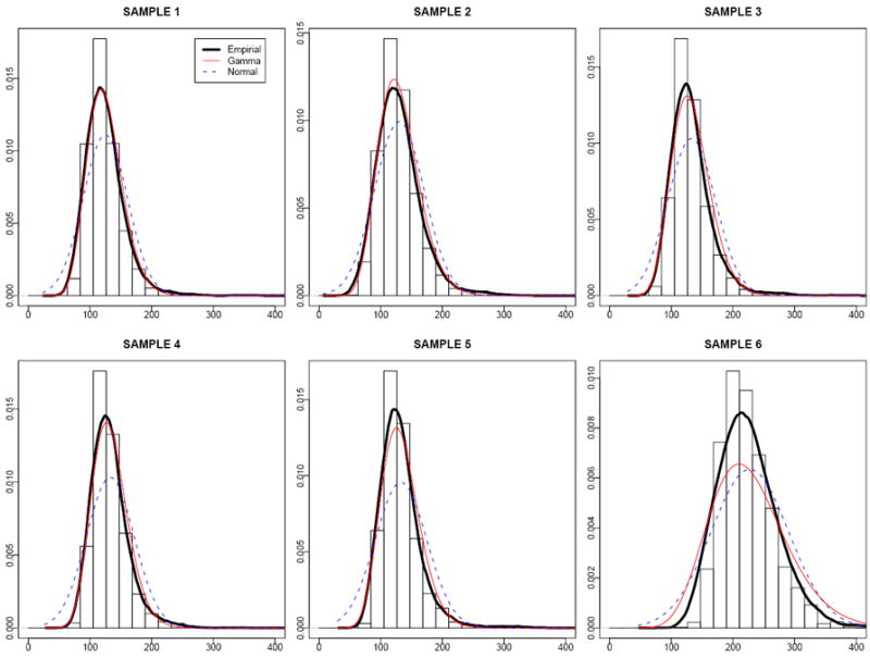
Histograms and density fittings of observed intensities for negative controls. Solid black, solid red and dashed blue lines are empirical, Gamma and Normal density curves, respectively. In sample 1-5 the Gamma density curves are closer to the empirical distributions than the normal ones, while in sample 6 they are similar.

2.2 Estimating parameters

The parameters θ, α and β need to be estimated from observed array data in order to adjust the background noise for gene probe signal intensity. Here we present the maximum likelihood estimators (MLE) that use the intensity data of all regular genes as well as negative controls.

For a regular gene i, the joint distribution of (X_i, Y_i) is:

$$\begin{array}{lll}f(x_i,y_i\mid \theta ,\alpha ,\beta )& =& \frac{1}{\theta }\exp (-\frac{x_i-y_i}{\theta })\frac{1}{\mathrm{\Gamma }(\alpha ){\beta }^{\alpha }}{y}_i^{\alpha -1}\exp (-\frac{y_i}{\beta })\\ & =& \frac{1}{\theta }\exp (-\frac{x_i}{\theta })\frac{1}{\mathrm{\Gamma }(\alpha ){\beta }^{\alpha }}{y}_i^{\alpha -1}\exp \left[-(\frac{1}{\beta }-\frac{1}{\theta })y_i\right].\end{array}$$

It is necessary to derive the marginal density function of X_i, which can be obtained from the joint density of (X_i, Y_i):

$$\begin{array}{lll}f(x_i\mid \theta ,\alpha ,\beta )& =& {\mathit{\int }}_0^{x_i}f(x_i,y_i\mid \theta ,\alpha ,\beta ){\mathit{dy}}_i\\ & =& {\mathit{\int }}_0^{x_i}\frac{1}{\theta }\exp (-\frac{x_i}{\theta })\frac{1}{\mathrm{\Gamma }(\alpha ){\beta }^{\alpha }}{y}_i^{\alpha -1}\exp \left[-(\frac{1}{\beta }-\frac{1}{\theta })y_i\right]{\mathit{dy}}_i\\ & =& \frac{1}{\theta }\exp (-\frac{x_i}{\theta })T(x_i;\theta ,\alpha ,\beta ),\end{array}$$

where

$$T(x_i;\theta ,\alpha ,\beta )=\{\begin{array}{ll}{\left(\frac{\theta }{\theta -\beta }\right)}^{\alpha }G(x_i;\alpha ,\frac{\theta \beta }{\theta -\beta })& \mathrm{if}\beta <\theta \\ \frac{1}{\mathrm{\Gamma }(\alpha ){\beta }^{\alpha }}{\mathit{\int }}_0^{x_i}{y}_i^{\alpha -1}\exp [-(\frac{1}{\beta }-\frac{1}{\theta })y_i]{\mathit{dy}}_i& \mathrm{if}\beta \ge \theta \end{array}.$$

Here G(x_i; α, θβ/(θ − β)) is the CDF of a Gamma distribution with parameters α and θβ/(θ − β).

Thus, the likelihood function of (θ, α, β) is

$$\begin{array}{lll}L(\theta ,\alpha ,\beta )& =& \prod _{i=1}^{N}f(x_i\mid \theta ,\alpha ,\beta )\cdot \prod _{j=1}^{M}f(x_{0j}\mid \alpha ,\beta )\\ & =& \prod _{i=1}^N\frac{1}{\theta }\exp (-\frac{x_i}{\theta })T(x_i;\theta ,\alpha ,\beta )\cdot \prod _{j=1}^M\frac{1}{\mathrm{\Gamma }(\alpha ){\beta }^{\alpha }}{x}_{0j}^{\alpha -1}\exp (-\frac{x_{0j}}{\beta }).\end{array}$$ (4)

Because only three parameters are involved, it is not hard to obtain the MLE of (θ, α, β) by numerical optimization algorithms provided by most statistical software. However, many such algorithms require initial values as the starting point. Rather than arbitrarily assigning initial search values, we can use the moment estimators from the data, as is described below.

The mean of X_0j is αβ and the variance is αβ². So the moment estimators of (α, β), based on the negative control data, are the solutions to

$$\begin{array}{ccc}\alpha \beta & =& \frac{{\sum }_{j=1}^M{X}_{0j}}{M}={\overline{X}}_0,\\ \alpha {\beta }^2& =& \frac{{\sum }_{j=1}^M{(X_{0j}-{\overline{X}}_0)}^2}{M}.\end{array}$$

Therefore,

$$\begin{array}{lll}\widehat{\alpha }& =& \frac{{\overline{X}}_0}{\widehat{\beta }},\\ \widehat{\beta }& =& \frac{{\sum }_{j=1}^M{(X_{0j}-{\overline{X}}_0)}^2}{{\sum }_{j=1}^M{X}_{0j}}.\end{array}$$

And the moment estimator of θ is

$$\widehat{\theta }=\frac{{\sum }_{i=1}^N{X}_i}{N}-\widehat{\alpha }\widehat{\beta }.$$

Moment estimators are sometimes biased. Nevertheless, in many cases they are good starting points for numerical algorithms in searching for maximum likelihood estimates.

3 Background Adjustment

In model based background adjustment methods, it is natural to use the conditional expectation of S_i given that the observed intensity is x_i. It is because this estimator minimizes the mean squared error, and it is used in many models like RMA and NMLE. Here, by applying the same idea we derive a new estimator, referred to as GMLE, of the true intensity after the background adjustment based on (1). First we need to derive the conditional distribution of S_i given X_i.

If β < θ,

$$f(s_i\mid x_i)=\frac{f(s_i,x_i)}{f(x_i)}=\frac{{(x_i-s_i)}^{\alpha -1}\exp [-(\frac{1}{\beta }-\frac{1}{\theta })(x_i-s_i)]}{{\left(\frac{\theta \beta }{\theta -\beta }\right)}^{\alpha }\mathrm{\Gamma }(\alpha )G(x_i;\alpha ,\frac{\theta \beta }{\theta -\beta })}.$$

It is not hard to see that (x_i−S_i)∣x_i (or Y_i∣x_i), when β < θ, is a truncated Gamma distribution in the interval (0, x_i] with parameters (α + 1) and θβ/(θ − β). So the estimate of the gene expression intensity, adjusted by the background noise given the observed value x_i, is

$$\begin{array}{lll}{\widehat{S}}_i& =& E(S_i\mid X_i=x_i)={\mathit{\int }}_0^{x_i}{s}_{i}f(s_i\mid x_i){\mathit{ds}}_i\\ & =& x_i-(\frac{\theta \beta }{\theta -\beta })\frac{\alpha G(x_i;\alpha +1,\frac{\theta \beta }{\theta -\beta })}{G(x_i;\alpha ,\frac{\theta \beta }{\theta -\beta })}.\end{array}$$

It is easy to calculate since it has a closed form solution. If, β ≥ θ,

$$\begin{array}{lll}f(s_i\mid x_i)& =& \frac{f(s_i,x_i)}{f(x_i)}\\ & =& \frac{{(x_i-s_i)}^{\alpha -1}\exp [-(\frac{1}{\beta }-\frac{1}{\theta })(x_i-s_i)]}{{\mathit{\int }}_0^{x_i}{y}_i^{\alpha -1}\exp [-(\frac{1}{\beta }-\frac{1}{\theta })y_i]{\mathit{dy}}_i}.\end{array}$$

And the background corrected intensity is:

$$\begin{array}{lll}{\widehat{S}}_i& =& E(S_i\mid X_i=x_i)={\mathit{\int }}_0^{x_i}{s}_{i}f(s_i\mid x_i){\mathit{ds}}_i\\ & =& x_i-\frac{{\mathit{\int }}_0^{x_i}{y}_i^{\alpha }\exp [-(\frac{1}{\beta }-\frac{1}{\theta })y_i]{\mathit{dy}}_i}{{\mathit{\int }}_0^{x_i}{y}_i^{\alpha -1}\exp [-(\frac{1}{\beta }-\frac{1}{\theta })y_i]{\mathit{dy}}_i}.\end{array}$$

The two integrals in the above formula have only one dimension and so they can be computed easily via numerical algorithms that are available in most statistical packages. And this method has been implemented in R package MBCB that will be submitted to Bioconductor. Details about the package can be found in Allen et al. (2009).

4 Simulation Studies

4.1 Parameter estimation

In the simulation we compare three methods, namely RMA, NMLE and GMLE, in the performance of parameter estimation of θ and the background adjustment. The gene expression intensities are simulated from exponential distributions with four settings of θ − 40, 60 and 100 − covering a range from relatively weak signals to very strong ones. For each value of θ, the noise is generated from Gamma distributions with parameters α ∈ {1.5, 2, 2.5} and β ∈ {20, 25, 30}, with the average noise level ranging from 30 to 75. For each setting of θ, α and β, 100 data sets, each of which contains 40,000 regular genes and 1,000 negative control intensities, are simulated from equation (1).

First we look at the estimation of θ, the average intensity of regular genes. The bias and the mean squared error (MSE) of θ̂ are summarized in table 1. Here since the true value of θ is known, the MSE can be computed over the 100 simulated data sets. We find that GMLE is unbiased with a small variance, while both RMA and NMLE are biased, although NMLE has much less bias than RMA. As θ increases, meaning the intensities of gene expression become stronger, the bias of NMLE becomes smaller, while RMA consistently gives significant under-estimates.

Table 1.

Mean and MSE of the Estimators of θ

θ	α	β	BIAS(θ̂)			MSE(θ̂)
			RMA	NMLE	GMLE	RMA	NMLE	GMLE
40	1.5	20	-30.4	4.6	0.0	925.0	21.5	0.3
		25	-29.6	6.9	0.0	874.8	48.0	0.4
		30	-28.6	9.5	0.0	819.4	91.3	1.0
	2	20	-29.9	5.6	-0.1	893.1	31.7	0.3
		25	-28.8	8.5	0.0	829.5	71.6	0.4
		30	-27.6	11.6	-0.1	765.0	134.5	0.9
	2.5	20	-29.5	6.4	-0.1	871.0	41.5	0.3
		25	-28.1	9.7	0.1	791.5	94.3	0.8
		30	-26.7	13.5	0.1	715.6	181.6	1.3
60	1.5	20	-47.0	3.4	-0.1	2209.4	11.4	0.2
		25	-46.4	5.0	-0.1	2149.5	25.7	0.4
		30	-45.6	7.0	-0.1	2076.7	49.1	0.5
	2	20	-46.7	4.0	0.0	2179.4	16.3	0.3
		25	-45.8	6.1	0.0	2099.8	37.9	0.4
		30	-44.8	8.4	-0.1	2010.4	71.2	0.5
	2.5	20	-46.4	4.7	0.0	2148.9	22.6	0.4
		25	-45.3	6.9	0.0	2050.7	48.6	0.4
		30	-44.1	9.7	-0.1	1949.3	94.8	0.7
100	1.5	20	-80.1	2.1	-0.1	6423.6	4.8	0.4
		25	-79.5	3.2	0.0	6320.0	11.0	0.5
		30	-78.9	4.7	0.1	6220.0	22.8	0.7
	2	20	-79.8	2.8	0.0	6370.1	8.0	0.5
		25	-79.1	4.1	0.0	6258.5	17.6	0.5
		30	-78.3	5.7	0.0	6134.5	32.6	0.7
	2.5	20	-79.5	3.2	0.0	6325.2	10.5	0.5
		25	-78.7	4.8	0.1	6200.7	23.8	0.6
		30	-77.8	6.5	0.0	6048.5	43.1	0.6

Next we look at the performance of the background adjustment for the three methods. After obtaining all parameter estimates, we can perform background noise correction and compare the resulting signal estimates with the true values that are known in the simulation study. For each simulated data set, we compute the MSE of noise adjusted intensities for all three methods, and report the average MSE over the 100 sample data sets as a measure of performance (figure 2). It can be seen that GMLE outperforms RMA by a large margin, and it is better than NMLE for each value of θ. For large θ, when the gene expression level is relatively high compared with the noise level, the difference between NMLE and GMLE is not big. However, as θ becomes smaller, the gain of using GMLE instead of NMLE is quite significant. Note that in the simulation we set the noise at fixed levels. In real data sets the estimated values of θ may have a wide range, for instance, from below 50 to over 200. And the variance of the noise typically increases as θ becomes large. Therefore, the improvement of GMLE can be substantial even for large values of θ if the signal to noise ratio is small.

Figure 2.

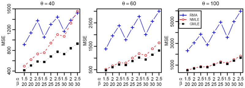
Average MSE of Noise Adjusted Intensities

4.2 Performance of detecting differentially expressed genes

Next we compare the performance of RMA, NMLE and GMLE in terms of detecting differentially expressed (DE) genes in a case-control experiment. Here the true expression level is assumed to follow an exponential distribution when the noise is simulated from a Gamma distribution. We simulate data from 4 BeadArrays, 2 for cases and 2 for controls. In each array we assume there are 40,000 probes to detect target gene expression levels and 1,500 non-specific probes as negative controls. Among the 40,000 probes, it is assumed that 4,000 are DE genes with 5 evenly distributed fold change levels (1.5, 2, 3, 4 and 5-fold) between the control and case groups. The true intensities of the controls are simulated from an Exponential distribution with θ = 40, and the noise is simulated from two settings, (a) Gamma(2.5, 30) and (b) Gamma(1.5, 20). The ROC curves are plotted in Figure 3. In both cases GMLE and NMLE outperform RMA. In setting (a) GMLE is a little better than NMLE and in (b) the difference of the two is larger, because the noise in (b) is more skewed than (a). In (b) the difference is not ignorable, especially within the interval between 0.1 and 0.3 of the false positive rate, where people usually are interested in choosing a cutoff point to maximize the true positive rate.

Figure 3.

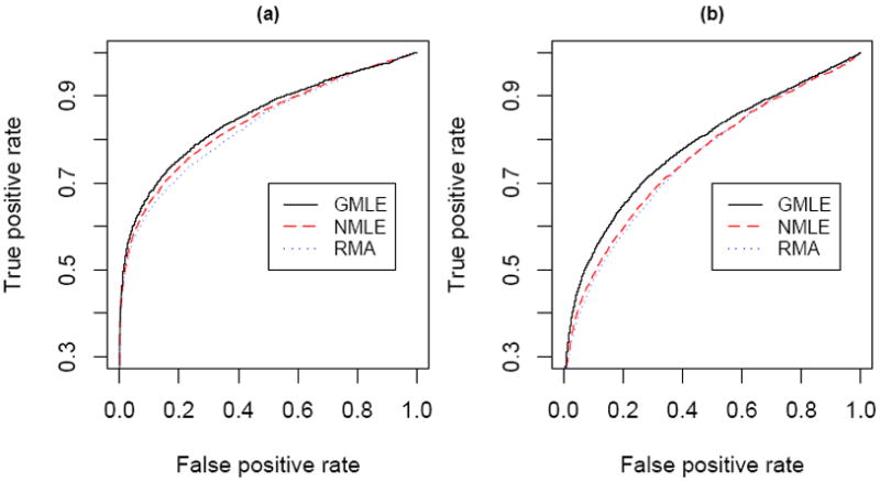
ROC of 3 methods when noise is Gamma

Further, to test the robustness of GMLE, additional simulations are done in the same setting as the above example except that the noise is simulated from a Lognormal(4,1) and a Normal(50,15) distribution, respectively. Note that the Lognormal distribution has a heavy right tail as displayed in panel (a) of Figure 4. So in the Lognormal case we set the signal mean to θ = 100 so that the signal-to-noise ratio is not too low. In this case the ROC curve, shown in Figure 4(b), suggests that GMLE is better than either RMA or NMLE. This is because the Gamma distribution, while allowing some right skewness, can provide a better approximation to Lognormal noises than the Normal distribution. On the other hand, when the noise is normally distributed, the ROC curve (Figure 4c) shows that GMLE is as good as NMLE, and both are better than RMA. This is not surprising because a Gamma distribution can also fit a symmetric distribution like the Normal quite well. Thus, the result suggests that the GMLE can be robust and flexible when the distribution of the noise is non-Gamma.

Figure 4.

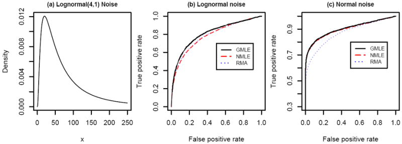
ROC of 3 methods when noise is Lognormal and normal

5 Real data examples

5.1 Lung cancer study

To explore the molecular mechanism of lung cancer pathogenesis after irradiation, we conducted microarray experiments to identify the genome-wide expression changes after irradiation on human bronchial epithelial cells (HBEC). The gene expression of HBEC samples were measured using the Illumina Whole Genome microarray HumanWG-6 V2 platform. There are 48791 genes and 1374 negative controls randomly allocated on each array. We conducted microarray experiments on 32 HBEC samples including 20 non-irradiated and 12 irradiated samples in order to identify differentially expressed genes between irradiated samples and non-radiated samples.

To evaluate the performance of different background correction methods, we compared false discovery rates (FDR) of identifying DE genes between radiated and non-radiated samples after using RMA, NMLE and GMLE background correction methods to all arrays in the study. After background correction, quantile normalization and log₂ transformation was used to preprocess the array data. Significance analysis of microarray (SAM) (Tusher et al., 2001) and a permutation-based false discovery rate approach (Xie et al., 2005) were used to identify DE genes between radiated and non-radiated samples. Figure 5 clearly shows that the proposed GMLE background correction method provides the lowest false discovery rate, and therefore this method is able to identify the greatest number of significant genes when controlling FDR at the same level.

Figure 5.

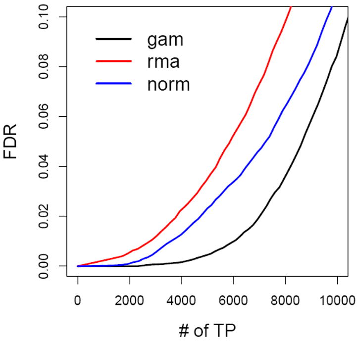
False discovery rates comparisons of lung cancer pathogenesis study.

5.2 Leukemia study

We also evaluated the different background correction methods by comparing the microarray experiments results with reverse transcriptase-polymerase chain reaction (RT-PCR) results in a leukemia study. The purpose of this microarray experiment is to identify DE genes between radiation induced leukemia mouse samples and control mouse samples. Illumina Mouse-6 V1 BeadChips have been used for this experiment, and the details of the experiments have been described in our previous publications (Xie et al., 2009; Ding et al., 2008). RT-PCR experiments are regarded as the gold standard to measure mRNA levels, and methods giving consistent results with RT-PCR are believed to be good methods. Figure 6 shows the comparison of microarray experiments with RT-PCR experiments for 14 randomly selected genes. We can see that the results from microarray experiments are very consistent with that from PCR. Background correction using GMLE leads to the most consistent results with RT-PCR with R² as 0.852 and the NMLE is slightly worse with R² as 0.838. The result shows that the GMLE method gives the best estimates for this experiment.

Figure 6.

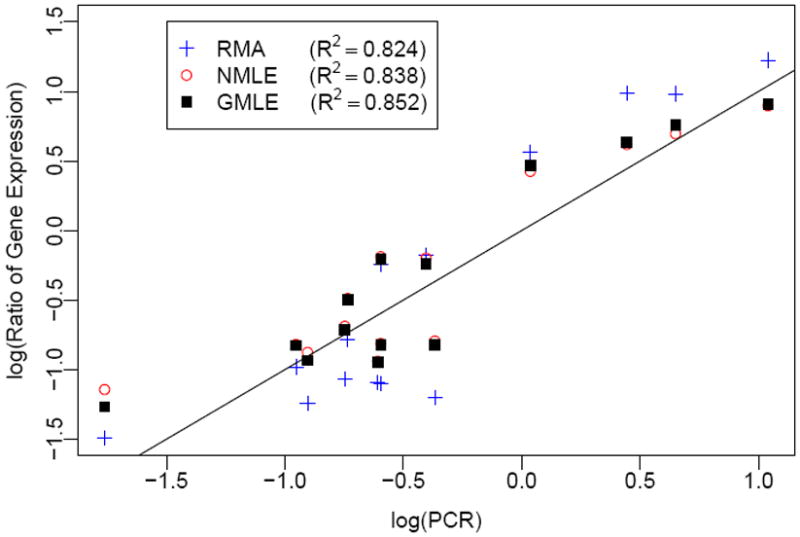
Scatter plot for the log₁₀ ratios (fold change) of gene expression between leukemia and normal tissues generated by RT-PCR and microarray with different background correction methods.

5.3 The Illumina spike-in experiment

We also use the data of Illumina spike-in experiment (Dunning et al., 2008) to test the three background adjustment methods. This experiment used 8 modified Mouse-6 version 1 BeadChips that were customized to include 33 extra bead types to target 9 bacterial and viral genes that are absent from the mouse genome. A series of samples were prepared by adding spiked mRNAs of the 9 genes with different predetermined concentrations to a common mouse background. And the 33 bead types were used to detect the spiked expressions of the 9 target genes. Each chip has 6 arrays. The first 4 chips were hybridized with samples having spikes at concentrations of 1000, 300, 100, 30, 10 and 3 pM, with one concentration on each array. The remaining 4 chips were hybridized with spikes at concentrations of 1, 0.3, 0.1, 0.03, 0.01 and 0 pM. More details and the download link about the data can be found in Dunning et al. (2008)

An exploration of the data shows that the signal are approximately distributed like an exponential random variable, and the noise from the negative control beads are fairly symmetrically distributed (Figure 7). So the model assumption seems to be satisfied, and one would expect that the GMLE would perform similarly as NMLE based on the previous simulation result in Figure 4(c). In Figure 8 the MA plot of log₂ transformed data from an array with spikes at 3 pM and another one with spikes at 0.3 pM. The x-axis is A = {log₂(ŝ_i) + log₂(ŝ_j)}/2 and the y-axis is M = log₂(ŝ_i) − log₂(ŝ_j). Red points in the graph represent the spike probes and their expected log-ratio value is around 3.2 as is marked by a horizontal dashed line. Panel (a) shows the data without background adjustment and panel (b), (c), (d) show RMA, NMLE, and GMLE, respectively. Without background adjustment, the M-values are under estimated and the range of M and A-values is small. After the background adjustment, the range of M and A-values increases in all of the three cases. And GMLE and NMLE seem to give unbiased estimates of the spikes, while RMA over estimates the M-values. As expected, GMLE is similar as NMLE, showing the flexibility of the GMLE as it can work well when the noise distribution is fairly symmetric.

Figure 7.

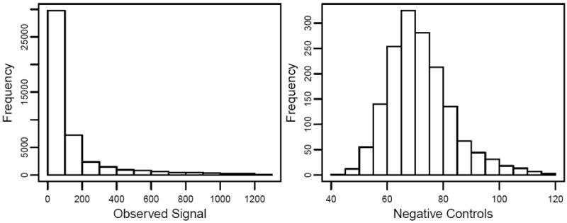
Histogram of observed signals and noises from the spike-in data.

Figure 8.

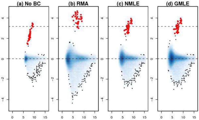
MA plot of spikes after BC correction by different methods.

6 Discussion

In this paper we have described a model based background correction method for Illumina BeadArray technology. This method takes advantage of a unique feature of BeadArrays, that is, the negative control beads that are designed to measure background noise. On the contrary, RMA does not utilize this information at all. And in other methods, like the one provided by Illumina that simply does subtraction, the information from the negative control beads would not help to improve, and in some cases even could impair the data quality because it could yield a large amount of negative gene expression levels that, unless being further processed by methods like VST, could not be used in further analysis.

The proposed method assumes the observed intensity comprised of a true signal reflecting the RNA expression level and a noise component that can be modeled by a Gamma distribution. Unlike naive approaches, the adjustment made via the use of this conditional expectation will not yield negative gene expression values. Furthermore, the Gamma distribution allows for large values of noise, and can work well when the noise is non-symmetrically distributed or can not be approximated by a Gaussian distribution. The negative control beads are used in several ways. They can be used to easily check the empirical distribution of noise, and can provide good estimates of distributions of parameters which can serve as starting point for numerical search algorithms in MLE. Furthermore, they are also included in the likelihood function, providing additional efficiency in parameter estimation and noise correction. In three real data examples, we demonstrated that using GMLE background correction can detect a greater number of significant DE genes when controlling for the same FDR, and the results are very consistent with RT-PCR results. Nonetheless, we should mention that there are cases when Gamma distributions might not be adequate (for example, sample 6 in Figure 1), requiring further efforts of developing more flexible methods. We would suggest to check the distribution of the noise, for example, fitting a Gamma density to the negative control data via MLE or moment estimation and looking at the Q-Q plot, before applying the background correction.

References

- Allen J, Chen M, Xie Y. Model-based background correction (MBCB): R methods and GUI for Illumina Bead-Array data. Journal of Cancer Science & Therapy. 2009;1(1):25–27. doi: 10.4172/1948-5956.1000004. [DOI] [PMC free article] [PubMed] [Google Scholar]
- Barnes M, Freudenberg J, Thompson S, Aronow B, Pavlidis P. Experimental comparison and cross-validation of the Affymetrix and Illumina gene expression analysis platforms. Nucleic Acids Research. 2005;33(18):5914–5923. doi: 10.1093/nar/gki890. [DOI] [PMC free article] [PubMed] [Google Scholar]
- Bolstad BM, Irizarry RA, Astrand M, Speed TP. A comparison of normalization methods for high density oligonucleotide array data based on variance and bias. Bioinformatics. 2003;19(2):185–193. doi: 10.1093/bioinformatics/19.2.185. [DOI] [PubMed] [Google Scholar]
- Ding L-H, Xie Y, Park S, Xiao G, Story MD. Enhanced identification and biological validation of differential gene expression via Illumina whole-genome expression arrays through the use of the model-based background correction methodology. Nucleic Acids Res. 2008;36(10):e58. doi: 10.1093/nar/gkn234. [DOI] [PMC free article] [PubMed] [Google Scholar]
- Dunning MJ, Barbosa-Morais NL, Lynch AG, Tavare S, Ritchie ME. Statistical issues in the analysis of Illumina data. BMC Bioinformatics. 2008;9:85. doi: 10.1186/1471-2105-9-85. [DOI] [PMC free article] [PubMed] [Google Scholar]
- Gunderson KL, Kruglyak S, Graige MS, Garcia F, Kermani BG, Zhao C, Che D, Dickinson T, Wickham E, Bierle J, Doucet D, Milewski M, Yang R, Siegmund C, Haas J, Zhou L, Oliphant A, Fan J-B, Barnard S, Chee MS. Decoding randomly ordered DNA arrays. Genome Research. 2004;14(5):870–877. doi: 10.1101/gr.2255804. [DOI] [PMC free article] [PubMed] [Google Scholar]
- Irizarry RA, Hobbs B, Collin F, Beazer-Barclay YD, Antonellis KJ, Scherf U, Speed TP. Exploration, normalization, and summaries of high density oligonucleotide array probe-level data. Biostatistics. 2003;4(2):249–264. doi: 10.1093/biostatistics/4.2.249. [DOI] [PubMed] [Google Scholar]
- Kuhn K, Baker SC, Chudin E, Lieu M-H, Oeser S, Bennett H, Rigault P, Barker D, McDaniel TK, Chee MS. A novel, high-performance random array platform for quantitative gene expression profiling. Genome Res. 2004;14(11):2347–2356. doi: 10.1101/gr.2739104. [DOI] [PMC free article] [PubMed] [Google Scholar]
- Li C, Wong WH. Model-based analysis of oligonucleotide arrays: expression index computation and outlier detection. Proc Natl Acad Sci U S A. 2001;98(1):31–36. doi: 10.1073/pnas.011404098. [DOI] [PMC free article] [PubMed] [Google Scholar]
- Lin SM, Du P, Huber W, Kibbe WA. Model-based variance-stabilizing transformation for Illumina microarray data. Nucleic Acids Res. 2008;36(2):e11. doi: 10.1093/nar/gkm1075. [DOI] [PMC free article] [PubMed] [Google Scholar]
- McGee M, Chen Z. Parameter estimation for the exponential-normal convolution model for background correction of Affymetrix genechip data. Statistical Applications in Genetics and Molecular Biology. 2006;5:24. doi: 10.2202/1544-6115.1237. [DOI] [PubMed] [Google Scholar]
- Ritchie ME, Silver J, Oshlack A, Holmes M, Diyagama D, Holloway A, Smyth GK. A comparison of background correction methods for two-colour microarrays. Bioinformatics. 2007;23(20):2700–2707. doi: 10.1093/bioinformatics/btm412. [DOI] [PubMed] [Google Scholar]
- Silver JD, Ritchie ME, Smyth GK. Microarray background correction: maximum likelihood estimation for the normal-exponential convolution. Biostatistics. 2009;10(2):352–363. doi: 10.1093/biostatistics/kxn042. [DOI] [PMC free article] [PubMed] [Google Scholar]
- Tusher VG, Tibshirani R, Chu G. Significance analysis of microarrays applied to the ionizing radiation response. Proc Natl Acad Sci U S A. 2001;98(9):5116–5121. doi: 10.1073/pnas.091062498. [DOI] [PMC free article] [PubMed] [Google Scholar]
- Wu Z, Irizarry RA, Gentleman R, Martinez-Murillo F, Spencer F. A model based background adjustment for oligonucleotide expression arrays. Journal of the American Statistical Association. 2004;99:909–917. [Google Scholar]
- Xie Y, Pan W, Khodursky AB. A note on using permutation-based false discovery rate estimates to compare different analysis methods for microarray data. Bioinformatics. 2005;21(23):4280–4288. doi: 10.1093/bioinformatics/bti685. [DOI] [PubMed] [Google Scholar]
- Xie Y, Wang X, Story M. Statistical methods of background correction for Illumina BeadArray data. Bioinformatics. 2009;25(6):751–757. doi: 10.1093/bioinformatics/btp040. [DOI] [PMC free article] [PubMed] [Google Scholar]