Problems With Risk Reclassification Methods for Evaluating Prediction Models

Abstract

For comparing the performance of a baseline risk prediction model with one that includes an additional predictor, a risk reclassification analysis strategy has been proposed. The first step is to cross-classify risks calculated according to the 2 models for all study subjects. Summary measures including the percentage of reclassification and the percentage of correct reclassification are calculated, along with 2 reclassification calibration statistics. The author shows that interpretations of the proposed summary measures and P values are problematic. The author's recommendation is to display the reclassification table, because it shows interesting information, but to use alternative methods for summarizing and comparing model performance. The Net Reclassification Index has been suggested as one alternative method. The author argues for reporting components of the Net Reclassification Index because they are more clinically relevant than is the single numerical summary measure.

Development of risk prediction models is a common and appealing area of research. Examples of well-known risk calculators are the Framingham Risk Score for 10-year risk of cardiovascular disease events (1) and the Gail model for breast cancer occurrence (2, 3). Risk models are attractive because they allow subjects to input data on their known risk factors and to calculate the corresponding risk value. This can be helpful for making decisions about treatment or other prevention strategies. Decisions are easiest, of course, when the calculated risk is very low or very high. Unfortunately, many risk calculators yield risk values that are intermediate for most persons. Therefore, enhancements to existing risk models are sought to improve their capacities to predict individual risk. Towards this aim, C-reactive protein has been added to the predictors in the Framingham Risk Score (4, 5), and breast density has been added to the predictors in the Gail model (6, 7).

How does one assess the performance of a risk prediction model? Measures that quantify performance are crucial, especially to gauge the improvement gained by addition of a new predictor to an existing set. It is widely appreciated that coefficients for predictors in a risk model are not adequate for the task of quantifying the population performance of the model for risk prediction (8). The population distribution of risk values provides a useful metric (9–12), since it displays the proportions of subjects deemed to be at low risk and/or at high risk by the model when thresholds are chosen to define low and/or high risk. Cook (13) suggests that when clinically meaningful categories of risk have been established by the medical community, such as they have been for cardiovascular disease, one should evaluate the proportions of subjects classified into each of the risk categories by the risk model. I agree with this suggestion.

Improvement in prediction performance might then be quantified by the increases in proportions of subjects falling into low and high risk categories by addition of a new predictor to a risk model. An alternative approach is the risk reclassification analysis strategy proposed by Cook and Ridker (14). This new analysis strategy has been promoted in clinically oriented journals (13–15) and is appearing in medical publications of research results (4, 16–18). However, it has received little attention from methodologists to date. My goal in this paper is to elucidate some properties of the risk reclassification approach described by Cook and Ridker (14) in order to better assess its role for evaluating the improvement in performance gained by adding a new predictor to a baseline prediction model. I also discuss some alternative strategies, including use of the Net Reclassification Index (19).

THE RISK RECLASSIFICATION ANALYSIS STRATEGY

Data for illustration are presented in Table 1. I generated these data from a specified risk model for the binary outcome, D, where D = 1 for an event and D = 0 for no event during a 10-year follow-up period. Details are provided in the Appendix. The underlying risk model that generated the data contained 3 predictors denoted by X, Y, and W, P(D = 1|X, Y, W). Suppose that X is the baseline predictor and Y is a new predictor. The predictor W exists, but we assume that it is as yet unknown, and therefore W is not part of the observed data set. The data for analysis are (D, X, Y), available for 10,000 persons. Given that data are only available on the variables (D, X, Y), we fit models to the observable risk functions, Risk(X) = P(D = 1|X) and Risk(X, Y) = P(D = 1|X, Y), the event probability given data only on predictor X and the event probability given data on both observed predictors (X, Y), respectively. We use logistic regression:

and

where logit (r) = log r/(1 − r). Results are shown in Table 2. Both models appear to fit the data well, with P values from 10-category Hosmer-Lemeshow goodness-of-fit statistics of 0.22 for the baseline model, Risk(X), and 0.15 for the enhanced model, Risk(X, Y). The coefficient for Y is highly statistically significant (P < 0.001).

Table 1.

Reclassification Table Comparing 10-Year Risk Strata From a Baseline Model That Includes Predictor X Only, Risk(X), With Strata From an Enhanced Model That Includes X and Y, Risk(X, Y)^a

Risk(X)	Risk(X, Y)
	0%–5%	5%–10%	10%–20%	>20%	Total
0%–5%	5,558	342	95	25	6,020
5%–10%	727	317	221	101	1,366
10%–20%	309	275	282	285	1,151
>20%	40	116	213	1,094	1,463
Total	6,634	1,050	811	1,505	10,000

^aNumbers of subjects are shown in the table. Data were simulated according to methods described in the Appendix.

Table 2.

Estimated Coefficients for Baseline and Enhanced Risk Models

Factor	Baseline Model		Enhanced Model
	Coefficient	SE	Coefficient	SE
Intercept	–3.67	0.07	–4.23	0.09
X	1.72	0.05	1.77	0.05
Y			1.01	0.05

Abbreviation: SE, standard error.

The objective of the analysis is to quantify the improvement in performance gained by adding Y to the baseline risk model that includes X alone. We use the 4 established risk categories for cardiovascular disease events (<5%, 5%–10%, 10%–20%, and >20%), in accordance with Cook and Ridker's analyses—categories derived from the guidelines of Adult Treatment Panel III (20). Each subject in the data set has 2 risk values calculated, one according to the baseline model and one according to the enhanced model. Table 1 shows the cross-classified values obtained using the 4 risk categories.

With baseline and enhanced risk models that appear to fit the observed data well, the risk reclassification analysis strategy is described as follows (14, p. 798):

• 1. Calculate the proportion of subjects classified into a different risk category by the enhanced model as compared with the baseline model. This is the proportion of subjects in off-diagonal cells. From Table 1, we see that there are 2,749 subjects reclassified, and we calculate

  
• 2. Determine the proportion of reclassified subjects that are “reclassified correctly.” Correct reclassification is deemed to have occurred for subjects in an off-diagonal cell if the observed proportion of events in that cell is closer to the category label for the enhanced model than to the category label for the baseline model. From Table 3, we see that this criterion holds for all off-diagonal cells. Correct reclassification appears to have occurred for all reclassified subjects.

  
• 3. Calculate 2 reclassification calibration statistics and their P values, one for the baseline model and one for the enhanced model. The reclassification calibration test statistic, RCC(model), compares the observed event rate in each interior cell with the average model-based risk for subjects in that cell:

  

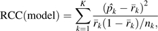
where ${\widehat{p}}_k$ is the observed event rate in the kth cell, ${\stackrel{-}{r}}_k$ is the average model-based risk for subjects in the kth cell, n_k is the number of subjects in the kth cell, and K is the number of interior cells in the table for which n_k ≥ 20 (K = 16 in Table 1). Observe that these statistics are different from the usual Hosmer-Lemeshow calibration test statistics that are based on the margins of the reclassification table.

Components of the test statistic for the baseline model, ${\widehat{p}}_k$ and ${\stackrel{-}{r}}_k$(baseline), and components of the test statistic for the enhanced model, ${\widehat{p}}_k$ and ${\stackrel{-}{r}}_k$(enhanced), are shown in Table 3 for our data. The test statistics are

and

which, when compared with the chi-squared distribution with K − 2 degrees of freedom as recommended by Cook and Ridker (14), yield P values of <0.00001 and 0.29, respectively. According to the proposed risk reclassification analysis strategy, the enhanced model is adequate but the baseline model is not.

Table 3.

Reclassification Table Showing Components of the Risk Reclassification Calibration and Event Rates (${\widehat{P}}_k$) Statistics, RCC(Baseline) and RCC(Enhanced), and Event Rates (${\widehat{p}}_k$) ^a

Risk(X)	Risk(X, Y)
	0%–5%		5%–10%		10%–20%		>20%		Total
	No.	%	No.	%	No.	%	No.	%	No.	%
0%–5%
nk	5,558		342		95		25		6,020
${\widehat{p}}_k$		1.30		7.89		11.58		16.00		1.89
${\stackrel{-}{r}}_k$(baseline)		1.49		3.12		3.39		3.86		1.62
${\stackrel{-}{r}}_k$(enhanced)		0.97		6.77		13.22		26.95		1.60
5%–10%
nk	727		317		221		101		1,366
${\widehat{p}}_k$		2.06		5.99		12.67		28.71		6.66
${\stackrel{-}{r}}_k$(baseline)		6.99		7.26		7.64		7.76		7.21
${\stackrel{-}{r}}_k$(enhanced)		2.53		7.12		13.93		28.32		7.34
10%–20%
nk	309		275		282		285		1,151
${\widehat{p}}_k$		1.94		7.27		13.48		29.82		12.95
${\stackrel{-}{r}}_k$(baseline)		13.34		13.99		14.67		15.11		14.26
${\stackrel{-}{r}}_k$(enhanced)		2.84		7.15		14.13		33.48		14.22
>20%
nk	40		116		213		1,094		1,463
${\widehat{p}}_k$		0.00		6.90		11.74		57.59		45.32
${\stackrel{-}{r}}_k$(baseline)		24.00		28.20		31.49		50.050		44.90
${\stackrel{-}{r}}_k$(enhanced)		3.20		7.57		14.71		56.21		44.86
Total
No. of subjects	6,634		1,050		811		1,505		10,000
${\widehat{p}}_k$		1.40		7.05		12.58		49.70		10.17
${\stackrel{-}{r}}_k$(baseline)		2.78		9.99		15.85		39.83		10.17
${\stackrel{-}{r}}_k$(enhanced)		1.24		7.06		14.12		49.55		10.17

Abbreviation: RCC, reclassification calibration.

^aIn the kth cell, n_k is the number of subjects, ${\widehat{p}}_k$ is the observed event rate, ${\stackrel{-}{r}}_k$(baseline) is the average baseline model risk, and ${\stackrel{-}{r}}_k$(enhanced) is the average enhanced model risk ${\widehat{p}}_k$. ${\stackrel{-}{r}}_k$(baseline) and ${\stackrel{-}{r}}_k$(enhanced) are shown as percentages.

SELF-FULFILLING RESULTS

I now show that some results from the Cook and Ridker risk reclassification analysis strategy are essentially predetermined, as long as standard statistical procedures are followed. Specifically, we assume that the new predictor, Y, has been determined to be a risk factor and that goodness-of-fit procedures have been carried out to ensure that the fitted models for P(D = 1|X) and P(D = 1|X, Y) approximate the observed data reasonably well. If one or both risk models do not appear to fit the observed data, there is no point in assessing risk reclassification, since those models are clearly not appropriate risk calculators.

Reclassification almost always appears “correct”

Consider an off-diagonal cell that we denote by AB, where a subject is in the cell if his calculated value for Risk(X) is in category A and that for Risk(X, Y) is in category B. Because the cell is defined by functions of X and Y, it follows mathematically that the anticipated event rate in cell AB is equal to the average of Risk(X, Y) for subjects in that cell:

(1)

A formal proof of equation 1 is:

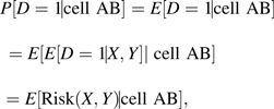where the second line follows because values of (X, Y) determine whether an observation is in cell AB, and the third line follows from the fact that E[D = 1|X, Y] = P(D = 1|X, Y) = Risk(X, Y). In real data, one uses a model for Risk(X, Y) that approximates the observed data frequencies P(D = 1|X, Y), implying that equation 1 holds to a good approximation.

Therefore, in large samples, the event rate in cell AB will approximate the average Risk(X, Y) for subjects in that cell. That average is necessarily in category B, because Risk(X, Y) is in category B and not in category A for all subjects in that cell. We conclude that reclassifications should always appear to be “correct” using the criterion set forth in item 2 of the reclassification analysis strategy, at least in large samples. Deviations can only occur due to sampling variability. Correspondingly, in the analysis of Table 1, we found that the criterion was satisfied by all off-diagonal cells. It is not surprising that we found 100% of reclassifications correct according to the Cook and Ridker criterion.

The reclassification calibration test of the enhanced model almost always accepts the null

Neither is it surprising that the reclassification calibration test of the enhanced model accepts the null hypothesis. This is because, assuming that preliminary analysis has shown a good fit of the observed data to the enhanced model, it follows that equation 1 holds to a good approximation. The equality in equation 1 in turn implies that the null hypothesis for the reclassification calibration test of the enhanced model always holds. Therefore, the test should only reject at the nominal rate, which is typically chosen to be 0.05. There is no point in performing this test.

The reclassification calibration test of the baseline model should reject the null

I contend that the reclassification calibration statistic for the baseline model is really a test statistic for an association between Y and D, controlling for X. To see this, consider first the simple setting in which the baseline model contains no covariates, so the baseline risk is the 10-year incidence of events for all subjects: Risk(X) = P(D = 1). Table 4 shows the reclassification table for this scenario. In this simple setting, the reclassification calibration statistic is exactly the same as the usual Pearson chi-squared statistic for association between the categorized version of Y and D; both are equal to 824.2 (P < 0.001). This is a general result that is proven algebraically in the Appendix.

Table 4.

Reclassification Table When the Baseline Model Contains No Covariates, So That the Fitted Baseline Risk = 10.17% for All Subjects

Baseline Risk = 10.17%	Risk(Y)
	<5%		5%–10%		10%–20%		>20%		Total
	No.	%	No.	%	No.	%	No.	%	No.	%
Subjects included	3,538		2,898		2,302		1,262		10,000
Event rate		3.02		7.42		13.42		30.59		10.17

When the baseline model is not constant, as in Table 1, I contend that the reclassification calibration statistic is at least conceptually similar to the Pearson chi-squared statistic but replaces the overall event rate in Table 4, P(D = 1) = 10.17%, with a version that conditions on the values of X for subjects in each cell. Moreover, observe that the null hypothesis tested by the reclassification calibration statistic of the baseline model is that, for each cell,

By equation 1 above, we can write this as

(2)

Therefore, if the reclassification calibration test of the baseline model is rejected, we must conclude that Risk(X, Y) ≠ Risk(X) for some subjects. However, this is simply the conclusion that Y is a risk factor after adjusting for X, a fact already established in preliminary analysis and which therefore does not need to be tested again.

Moreover, observe that the null hypothesis in equation 2 cannot hold for off-diagonal cells, since the average on the left-hand side must be in risk category B, while that on the right-hand side must be in risk category A. Therefore, in large samples, the reclassification calibration test of the baseline model must reject its null hypothesis, at least when there are observations in some off-diagonal cells. In practice, with finite sample sizes, it is possible for the baseline model reclassification calibration test not to reject while the test in preliminary analysis shows Y to be a risk factor. However, this can only be due to sampling variability and lower power for the reclassification calibration test compared with efficient likelihood-based procedures that are typically used to test whether Y is a risk factor in preliminary analyses.

In summary, if Y has been determined to be a risk factor, with a sufficiently large sample size the reclassification calibration test of the baseline model will be rejected. There is no point in performing this test.

CAUTIONARY REMARKS

True underlying risk

Cook (15) motivated the development of the new risk reclassification analysis strategy in part by distinguishing between risk prediction research and diagnostic research. In the diagnostic setting, the event has already occurred, whereas in the prediction setting, an event may or may not occur in the future. Cook argues that the stochastic nature of that occurrence must be recognized. A subject's “true underlying risk,” denoted by π, is his inherent probability of a future event. In general, this seems like a nebulous entity. Nevertheless, this underlying risk may be different from the observable risks that are well-defined conditional probabilities, Risk(X) = P(D = 1|X) and Risk(X, Y) = P(D = 1|X, Y), modeled by the baseline and enhanced risk prediction models, respectively. Specifically, Risk(x) is defined as a frequency, namely the event rate among subjects with X = x, while Risk(x, y) is defined as the event rate in the subset of those subjects with Y = y as well as X = x.

The “true underlying risk,” π, will be different from the observable risk, Risk(X, Y), which is a function of observed predictors (X, Y), if there exist additional, possibly unmeasured or unknown variables that are predictive. The data set we simulated includes 1 additional predictive variable, W, and the true underlying risks, π = P(D = 1|X, Y, W), are known to us because we specified them in order to generate the outcome data. For analysis, however, we have assumed that we have available only D, X, and Y.

The algorithm for determining “correct reclassification” is not correct

We can compare true underlying risk values with the enhanced model risk values, Risk(X, Y), for our simulated data. Specifically, we compared risk category assignments made with values of π = P(D = 1|X, Y, W) with those made using values of Risk(X, Y) for subjects in the reclassified cells of Table 1. Of the 2,749 reclassified subjects, we found that 919 risk category assignments (33.4%) made on the basis of Risk(X, Y) were incorrect, in the sense that they were different from the risk category assigned to them on the basis of their “true underlying risk,” π. In contrast, the risk reclassification analysis strategy concludes that 100% of reclassifications are correct. The criterion stipulated for identifying reclassifications as correct or not in item 2 of the strategy is simply not valid.

Inference about true underlying risk is not possible

Although the notion of true underlying risk is interesting, underlying risk cannot be revealed by data, except in extremely predictable scenarios such as those involving certain Mendelian disorders. Given only observed variables (X, Y, D), one cannot know whether there exists an unmeasured predictive marker, W, or not. If not, (X, Y) contains all predictive information, and true underlying risk is the same as Risk(X, Y). On the other hand, in our data, true underlying risk is P(D = 1|X, Y, W), which is very different from Risk(X, Y) = P(D = 1|X, Y) for a large number of people, because W is highly predictive.

Using the observed variables (X, Y, D), one can only make inference about the conditional probabilities, Risk(X, Y) = P(D = 1|X, Y), not specifically about π. Interestingly, we can also think of Risk(X, Y) as averaging true underlying risk among subjects defined by X and Y,

Thus, we can make inference about averages of underlying risk among subpopulations defined by X and Y, but beyond that, true underlying risk cannot be identified from data.

Much reclassification does not imply improvement

It is tempting to consider reclassification of risk for substantial numbers of subjects as evidence of improved risk prediction with the enhanced model (21). However, Cook has repeatedly emphasized that a large number of reclassified subjects does not necessarily imply improved performance for the enhanced model over the baseline model (14, 22). Consider, for example, that the amount of reclassification is determined in part by the numbers and choices of risk categories. Correlation between risk predictors also affects reclassification percentage (23).

In our data, approximately 28% of subjects were reclassified, yet the number of subjects classified into the highest risk category increased only slightly, from 1,463 to 1,505. If the objective is to identify high-risk subjects, the addition of Y to the baseline predictors did not help, despite substantial reclassification. The number of subjects classified into the lowest risk category did increase, but only by 10.2% (614/6,020 = 10.2%).

The fact that substantial reclassification can occur in the absence of substantial improvement in risk model performance has also been observed in other data sets. For example, Gail (21) found that adding 7 single nucleotide polymorphisms to a breast cancer risk model resulted in substantial risk reclassification but negligible gain in terms of a cost-benefit analysis.

BETTER METHODS FOR EVALUATING PREDICTION MODELS

This paper is not intended to provide comprehensive guidance on how to evaluate and compare the performances of risk prediction models. There is a growing body of literature on the topic, and I recommend several papers to the interested reader (9, 10, 19, 23–28). Instead, the focus here is on use of the Cook and Ridker (14) risk reclassification analysis strategy defined in items 1–3 above. I have noted some major concerns that I have about interpretations for the percentage of reclassification, the percentage of correct reclassification, and the 2 reclassification calibration statistics. My discussion assumes that fitted risk models appear to approximate the observed data reasonably well, as assessed by standard goodness-of-fit procedures. Assessment of goodness of fit is a precursor to evaluating risk reclassification (14, 16, 23). In my example, simple linear logistic models fitted the observed data well, but in practice more complex models are often needed. I also ignored potential biases due to evaluating model performance in the same data used to fit the risk models. Ideally, one would use independent data sets to fit models and assess performance.

Certainly, the cross-tabulation itself is not problematic. It can be interesting to examine the extent to which individuals' risk categories change (or not) by adding a new predictor to a baseline model. In order to compare the population performance of the enhanced model with that of the baseline model, however, the margins of the risk reclassification table are more relevant than are the interior cells of the table, because the margins show the net increases in numbers of subjects classified into high or low risk categories (23). Moreover, I and others have argued for displaying the net changes separately for subjects with and without events (19, 23). We see from the margins of Table 5 that of the 1,017 subjects with events, the proportions in the 4 risk categories changed from (11.2%, 9.0%, 14.7%, 65.2%) with use of the baseline model to (9.1%, 7.3%, 10.0%, 73.6%) with use of the enhanced model, a shift towards the higher risk categories. In particular, we see that of subjects who had events, 8.4% more (73.6 – 65.2 = 8.4%) would have been classified in the highest risk category at time 0 by including Y in the risk model. The margins of Table 5 also show that for the 8,983 subjects without events, the proportions in the 4 risk categories changed from (65.8%, 14.2%, 11.2%, 8.9%) with use of the baseline model to (72.8%, 10.9%, 7.9%, 8.4%) with use of the enhanced model, a shift towards the lower risk categories. Of subjects who did not have events, 7.0% more (72.8 – 65.8 = 7.0%) would have been classified in the lowest risk category at time 0 by including Y in the risk model.

Table 5.

Event and Nonevent Reclassification

Risk(X)	Risk(X, Y)
	0%–5%	5%–10%	10%–20%	>20%	Total
Events
0%–5%	72	27	11	4	114
5%–10%	15	19	28	29	91
10%–20%	6	20	38	85	149
>20%	0	8	25	630	663
Total	93	74	102	748	1,017
Nonevents
0%–5%	5,486	315	84	21	5,906
5%–10%	712	298	193	72	1,275
10%–20%	303	255	244	200	1,002
>20%	40	108	188	464	800
Total	6,541	976	709	757	8,983

The Net Reclassification Index (NRI) is a popular statistic that is computed from the event and nonevent reclassification table (Table 5). For subjects with events, it counts the proportion that moved to a higher risk category, less the number that moved to a lower risk category. That is, it counts the proportion above the diagonal in the table versus the proportion below the diagonal—for our data, (184 − 74)/1,017 = 0.108. Similarly, for subjects without events, it counts the proportion shifted to a lower risk category, which is the proportion below the diagonal versus the proportion above the diagonal: (1,606 − 885)/8,983 = 0.080. It then sums the 2 components. For our data, therefore, the NRI is 0.188. Interpretation of the NRI is problematic, however, partly because the summation of the 2 components masks the relative contributions of each. An NRI of 0.188 may be due, at one extreme, to 18.8% of subjects with events moving to a higher risk category without any shift for subjects without events or, at the other extreme, to 18.8% of subjects without events moving to a lower risk category without any shift for subjects with events; or it may be due to approximately equal proportions of events and nonevents moving to improved risk categories, as was the case for our data. I suggest at least reporting the 2 components of the NRI separately, the event NRI (10.8%) and the nonevent NRI (8.3%). Better still would be to report the changes in proportions of subjects in each of the risk categories. The changes in the distribution of risk categories for subjects with and without events are (−2.1%, −1.7%, −4.6%, 8.4%) and (7.1%, −3.3%, −3.3%, −0.5%), respectively. I find this summary more informative because the risk categories are acknowledged explicitly. For example, if one is concerned primarily with the highest and lowest risk categories, we see that for subjects with events the enhanced model improves the proportions of them in the highest and lowest risk categories, and improvement is also seen in both risk category proportions for subjects without events.

Finally, I reiterate that analyses using risk categories are predicated on the existence of risk categories that have been defined on the basis of sound, clinically motivated criteria. Unfortunately, the existence of categories that are widely agreed upon is more the exception than the rule in practice. When risk categories have not been defined on the basis of sound, clinically motivated criteria, the continuous distributions of Risk(X) and Risk(X, Y) can be presented instead of categorized versions (10, 24). These allow viewers to overlay various risk categories and ideally clinically meaningful risk categories that may be developed post hoc. Scatterplots of Risk(X, Y) versus Risk(X) can be used instead of cross-tabulations to avoid the use of specific risk categories in presentation.

Glossary

Abbreviation

NRI

Net Reclassification Index

Appendix Table 1.

Appendix Table 1.

Notation used to demonstrate that the Pearson chi-squared statistic is equal to the risk reclassification statistic for the baseline risk model^a

	Category for Risk(Y)
	1	2	. . .	K	Total
Events	O1	O2	. . .	OK	O = ∑Ok
Nonevents	n1 − O1	n2 − O2	. . .	nK − OK	n − ∑Ok
No. of subjects	n1	n2	. . .	nK	n = ∑nk
Event rate	$p_1=\frac{O_1}{n_1}$	$p_2=\frac{O_2}{n_2}$	. . .	$p_K=\frac{O_K}{n_K}$	$p=\frac{\mathrm{\Sigma }{O}_k}{n}$

^aThe upper 2 rows show notation corresponding to the Pearson chi-squared statistic. The lower 2 rows show notation corresponding to the risk reclassification statistic. There is only 1 category for the baseline risk.

Data for illustration

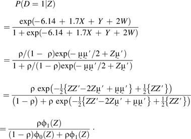
I generated data on 4 variables, {D, X, Y, W}, for 10,000 subjects, so that the binary outcome D is equal to 1 with probability P(D = 1|X, Y, W), where

My method for generating data, described below, implies that logistic regression models also hold for the observable risk functions, Risk(X, Y) = P(D = 1|X, Y) and Risk(X) = P(D = 1|X):

and

For the simulation algorithm, I first created a population covariate distribution by simulating 900,000 observations with (X, Y, W) from independent standard normal distributions and 100,000 observations with (X, Y, W) from independent normal distributions with mean values of (1.7, 1.0, 2.0) and standard deviations of (1, 1, 1). I then generated D with binomial probability P(D = 1|X, Y, W), given in the expression above, and selected 10,000 subjects at random for the study cohort.

I prove below that this procedure gives rise to data with conditional distributions P(X, Y, W|D = 1) and P(X, Y, W|D = 0) that are multivariate normal with identity covariance matrices and means of (1.7, 1, 2) and (0, 0, 0), respectively. From this it follows that the conditional distributions of (X, Y), P(X, Y|D = 1) and P(X, Y|D = 0), are bivariate normal with identity covariance matrices and that the conditional distributions of X, P(X|D = 1) and P(X|D = 0), are normal with variance 1. It follows from classic discriminant analysis that when data are (multivariate) normal with equal variance-covariance in 2 classes, D = 0 and D = 1, the corresponding risk functions are linear logistic. This follows from a simple application of Bayes' theorem and some algebra.

Conditional distributions of (X, Y, W)

To simplify notation, we use Z for the vector (X, Y, W), $\underset{~}{\text{μ}}$ for (1.7, 1.0, 2.0), and ρ for 0.1. The distribution of Z is written as p(Z) = ρϕ₀(Z) + (1 − ρ)ϕ₁(Z), where ϕ₀ and ϕ₁ are trivariate normal distributions with identity variance-covariance matrix and means (0, 0, 0) and $\underset{~}{\mu }$, respectively. Observe that $\log (\text{ρ/(}1-\text{ρ}))-\underset{~}{\mu }\underset{~}{\mu }\text{/2}=-\mathrm{6.14.}$

Therefore,

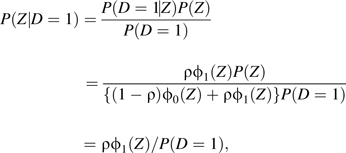because P(Z) = (1 − ρ)ϕ₀(Z) + ρϕ₁(Z) according to the procedure generating Z.

It follows by integrating P(D = 1|Z) over Z that P(D = 1) = ρ, so the result P(Z|D = 1) = ϕ₁(Z) follows. A similar proof shows P(Z|D = 0) = ϕ₀(Z).

The raw data are available on the Web site of the Diagnostic and Biomarkers Statistical Center (http://labs.fhcrc.org/pepe/dabs/datasets.html).

Risk classification with no baseline covariates

I show that the risk reclassification calibration statistic is equal to the Pearson chi-squared statistic for association in the simple setting where the baseline risk is the overall event rate for all subjects. Appendix Table 1 defines the relevant notation. Let E_k (and n_k − E_k) be the expected events (and nonevents) in the kth Risk(Y) category. Under the null, E_k = n_kp (and n_k − E_k = n_k (1 − p)). We write

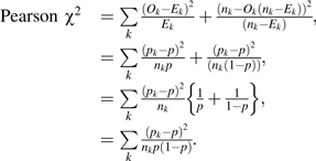This is identical to the expression for the reclassification calibration test of the baseline model when the baseline model assigns all subjects the same risk; p = the overall event rate, that is, when there are no baseline covariates.

References

- 1.Wilson PW, D'Agostino RB, Levy D, et al. Prediction of coronary heart disease using risk factor categories. Circulation. 1998;97(18):1837–1847. doi: 10.1161/01.cir.97.18.1837. [DOI] [PubMed] [Google Scholar]
- 2.Gail MH, Brinton LA, Byar DP, et al. Projecting individualized probabilities of developing breast cancer for white females who are being examined annually. J Natl Cancer Inst. 1989;81(24):1879–1886. doi: 10.1093/jnci/81.24.1879. [DOI] [PubMed] [Google Scholar]
- 3.Gail MH, Costantino JP. Validating and improving models for projecting the absolute risk of breast cancer. J Natl Cancer Inst. 2001;93(5):334–335. doi: 10.1093/jnci/93.5.334. [DOI] [PubMed] [Google Scholar]
- 4.Ridker PM, Buring JE, Rifai N, et al. Development and validation of improved algorithms for the assessment of global cardiovascular risk in women: the Reynolds Risk Score. JAMA. 2007;297(6):611–619. doi: 10.1001/jama.297.6.611. [DOI] [PubMed] [Google Scholar]
- 5.Ridker PM, Paynter NP, Rifai N, et al. C-reactive protein and parental history improve global cardiovascular risk prediction: the Reynolds Risk Score for men. Circulation. 2008;118(22):2243–2251. doi: 10.1161/CIRCULATIONAHA.108.814251. [DOI] [PMC free article] [PubMed] [Google Scholar]
- 6.Chen J, Pee D, Ayyagari R, et al. Projecting absolute invasive breast cancer risk in white women with a model that includes mammographic density. J Natl Cancer Inst. 2006;98(17):1215–1226. doi: 10.1093/jnci/djj332. [DOI] [PubMed] [Google Scholar]
- 7.Barlow WE, White E, Ballard-Barbash R, et al. Prospective breast cancer risk prediction model for women undergoing screening mammography. J Natl Cancer Inst. 2006;98(17):1204–1214. doi: 10.1093/jnci/djj331. [DOI] [PubMed] [Google Scholar]
- 8.Pepe MS, Janes H, Longton G, et al. Limitations of the odds ratio in gauging the performance of a diagnostic, prognostic, or screening marker. Am J Epidemiol. 2004;159(9):882–890. doi: 10.1093/aje/kwh101. [DOI] [PubMed] [Google Scholar]
- 9.Stern RH. Evaluating new cardiovascular risk factors for risk stratification. J Clin Hypertens (Greenwich) 2008;10(6):485–488. doi: 10.1111/j.1751-7176.2008.07814.x. [DOI] [PMC free article] [PubMed] [Google Scholar]
- 10.Pepe MS, Feng Z, Huang Y, et al. Integrating the predictiveness of a marker with its performance as a classifier. Am J Epidemiol. 2008;167(3):362–368. doi: 10.1093/aje/kwm305. [DOI] [PMC free article] [PubMed] [Google Scholar]
- 11.Huang Y, Sullivan Pepe M, Feng Z. Evaluating the predictiveness of a continuous marker. Biometrics. 2007;63(4):1181–1188. doi: 10.1111/j.1541-0420.2007.00814.x. [DOI] [PMC free article] [PubMed] [Google Scholar]
- 12.Yang Q, Liu T, Valdez R, et al. Improvements in ability to detect undiagnosed diabetes by using information on family history among adults in the United States. Am J Epidemiol. 2010;171(10):1079–1089. doi: 10.1093/aje/kwq026. [DOI] [PMC free article] [PubMed] [Google Scholar]
- 13.Cook NR. Use and misuse of the receiver operating characteristic curve in risk prediction. Circulation. 2007;115(7):928–935. doi: 10.1161/CIRCULATIONAHA.106.672402. [DOI] [PubMed] [Google Scholar]
- 14.Cook NR, Ridker PM. Advances in measuring the effect of individual predictors of cardiovascular risk: the role of reclassification measures. Ann Intern Med. 2009;150(11):795–802. doi: 10.7326/0003-4819-150-11-200906020-00007. [DOI] [PMC free article] [PubMed] [Google Scholar]
- 15.Cook NR. Statistical evaluation of prognostic versus diagnostic models: beyond the ROC curve. Clin Chem. 2008;54(1):17–23. doi: 10.1373/clinchem.2007.096529. [DOI] [PubMed] [Google Scholar]
- 16.Paynter NP, Cook NR, Everett BM, et al. Prediction of incident hypertension risk in women with currently normal blood pressure. Am J Med. 2009;122(5):464–471. doi: 10.1016/j.amjmed.2008.10.034. [DOI] [PMC free article] [PubMed] [Google Scholar]
- 17.Lauer MS, Pothier CE, Magid DJ, et al. An externally validated model for predicting long-term survival after exercise treadmill testing in patients with suspected coronary artery disease and a normal electrocardiogram. Ann Intern Med. 2007;147(12):821–828. doi: 10.7326/0003-4819-147-12-200712180-00001. [DOI] [PubMed] [Google Scholar]
- 18.Tice JA, Cummings SR, Smith-Bindman R, et al. Using clinical factors and mammographic breast density to estimate breast cancer risk: development and validation of a new predictive model. Ann Intern Med. 2008;148(5):337–347. doi: 10.7326/0003-4819-148-5-200803040-00004. [DOI] [PMC free article] [PubMed] [Google Scholar]
- 19.Pencina MJ, D'Agostino RB Sr, D'Agostino RB, Jr, et al. Evaluating the added predictive ability of a new marker: from area under the ROC curve to reclassification and beyond. Stat Med. 2008;27(2):157–172. doi: 10.1002/sim.2929. [DOI] [PubMed] [Google Scholar]
- 20.Expert Panel on Detection. Evaluation, and Treatment of High Blood Cholesterol in Adults. Executive summary of the Third Report of The National Cholesterol Education Program (NCEP) Expert Panel on Detection, Evaluation, and Treatment of High Blood Cholesterol in Adults (Adult Treatment Panel III) JAMA. 2001;285(19):2486–2497. doi: 10.1001/jama.285.19.2486. [DOI] [PubMed] [Google Scholar]
- 21.Gail MH. Value of adding single-nucleotide polymorphism genotypes to a breast cancer risk model. J Natl Cancer Inst. 2009;101(13):959–963. doi: 10.1093/jnci/djp130. [DOI] [PMC free article] [PubMed] [Google Scholar]
- 22.Cook NR. Comment: measures to summarize and compare the predictive capacity of markers. Int J Biostat. 2010;6(1) doi: 10.2202/1557-4679.1257. Article 22. ( http://www.bepress.com/ijb/vol6/iss1/22). (doi: 10.2202/1557-4679.1257) [DOI] [PMC free article] [PubMed] [Google Scholar]
- 23.Janes H, Pepe MS, Gu W. Assessing the value of risk predictions by using risk stratification tables. Ann Intern Med. 2008;149(10):751–760. doi: 10.7326/0003-4819-149-10-200811180-00009. [DOI] [PMC free article] [PubMed] [Google Scholar]
- 24.Gu W, Pepe M. Measures to summarize and compare the predictive capacity of markers. Int J Biostat. 2009;5(1) doi: 10.2202/1557-4679.1188. Article 27. ( http://www.bepress.com/ijb/vol5/iss1/27). (doi: 10.2202/1557-4679.1188) [DOI] [PMC free article] [PubMed] [Google Scholar]
- 25.Steyerberg EW, Vickers AJ, Cook NR, et al. Assessing the performance of prediction models: a framework for traditional and novel measures. Epidemiology. 2010;21(1):128–138. doi: 10.1097/EDE.0b013e3181c30fb2. [DOI] [PMC free article] [PubMed] [Google Scholar]
- 26.Steyerberg EW. Clinical Prediction Models: A Practical Approach to Development, Validation, and Updating. New York, NY: Springer Publishing Company; 2009. [Google Scholar]
- 27.Vickers AJ, Elkin EB. Decision curve analysis: a novel method for evaluating prediction models. Med Decis Making. 2006;26(6):565–574. doi: 10.1177/0272989X06295361. [DOI] [PMC free article] [PubMed] [Google Scholar]
- 28.Pepe MS, Gu JW, Morris DE. The potential of genes and other markers to inform about risk. Cancer Epidemiol Biomarkers Prev. 2010;19(3):655–665. doi: 10.1158/1055-9965.EPI-09-0510. [DOI] [PMC free article] [PubMed] [Google Scholar]