From atomistic modeling to excitation transfer and two-dimensional spectra of the FMO light-harvesting complex

Abstract

The experimental observation of long-lived quantum coherences in the Fenna-Matthews-Olson (FMO) light-harvesting complex at low temperatures has challenged general intuition in the field of complex molecular systems and provoked considerable theoretical effort in search for explanations. Here we report on room-temperature calculations of the excited-state dynamics in FMO using a combination of molecular dynamics simulations and electronic structure calculations. Thus we obtain trajectories for the Hamiltonian of this system which contains time-dependent vertical excitation energies of the individual bacteriochlorophyll molecules and their mutual electronic couplings. The distribution of energies and couplings are analyzed together with possible spatial correlations. It is found that in contrast to frequent assumptions the site energy distribution is non-Gaussian. In a subsequent step, averaged wave packet dynamics is used to determine the exciton dynamics in the system. Finally, with the time-dependent Hamiltonian linear and two-dimensional spectra are determined. The thus obtained linear absorption lineshape agrees well with experimental observation and is largely determined by the non-Gaussian site energy distribution. The two-dimensional spectra are in line with what one would expect by extrapolation of the experimental observations at lower temperatures and indicate almost total loss of long-lived coherences.

Introduction

In photosynthesis the energy of sunlight is converted into chemical energy. Light harvesting and charge separation are the primary steps in this process. Specific pigment-protein aggregates, the so-called light-harvesting (LH) complexes, have the function of absorbing light and transporting the energy to the photosynthetic reaction center (RC). Within the RC the excitation is subsequently converted into charge separation.¹ Many of the structural and functional details of these protein complexes have been elucidated already.^2–4

One of the extensively studied LH systems is the Fenna-Matthews-Olson (FMO) complex of green sulphur bacteria.⁵ For the bacterium Prosthecochloris aestuarii the crystal structure was already solved three decades ago,⁶ the first time that this was achieved for a pigment-protein complex. Meanwhile the structure has been characterized at atomic resolution 1.9 Å.⁷ Recently, the structure of the FMO complex of Chlorobaculum tepidum has been determined as well.⁸ Under physiological conditions, the FMO complex forms a homotrimer consisting of eight bacteriochlorophyll-a (BChl a) molecules per monomer. The existence of an eighth BChl molecule in the structure of each monomer has been shown only recently;⁸ many earlier studies refer to just seven BChls per monomer. The biological function of the FMO trimer is to transfer excitation energy from the chlorosome, i.e., the main LH antenna system of green sulfur bacteria, to the RC, which is embedded into the membrane.⁵ The optical properties of FMO complexes together with the experimental and theoretical approaches were reviewed recently in great detail.⁵ We note that the photophysical investigations published thus far were performed on FMO trimers rather than monomers. Nevertheless, additional studies of the monomeric system as performed here yield insight into properties also of the trimeric arrangement.

A few years ago, using two-dimensional correlation spectroscopy the Fleming group reported evidence for coherent energy-transfer dynamics in FMO.^9,10 Because of the unexpectedly long coherence times of around 700 fs at 77 K, the findings provoked a large number of further studies, both experimental and theoretical ones. By now, similar coherence times have been shown to arise at higher temperatures¹¹ for the same FMO complex of Chlorobaculum tepidum, for a photo-synthetic complex of marine algae at ambient temperature¹² as well as in conjugated polymers.¹³ It has been suggested that the long-lived coherence is due to correlations of site energies fluctuations.¹⁴ A few publications have investigated the possible effect of correlated motions.^15–22 In earlier simulations for LH systems combined with semiemperical electronic structure calculations, reported by several of the present authors, we did not find spatial correlation in the time dependence of the site energies.^23,24 Alternative suggestions that the long-lived coherences originate from interferences of different quantum pathways have been put forward recently.^25,26

In this paper, we aim to give a parameter-free calculation of the excited-state dynamics and the linear and two-dimensional spectra for FMO. Our method is based on a combination of classical molecular dynamics (MD) and electronic structure calculations. Using MD one can model complete LH systems.^23,27 Nonetheless, MD simulations are neither able to describe the optical properties of such systems nor the excitation transfer therein. For such description, one has to couple electronic structure calculations to the classical simulations.^23,27–31 Even for semiempirical methods, the determination of the electronic structure of the complete system over time is computationally expensive. Therefore, one usually adopts a subsystem-based approach in which the excitation energy for each individual BChl is calculated separately. In addition to the individual excitation energies, one needs to determine the electronic coupling between the subsystems. To record the effect of the thermal fluctuations on the energy transfer dynamics and optical properties, the quantum chemistry calculations of the excitation energies and the electronic couplings have to be performed along an MD trajectory.^{23,27,30–33} To calculate the vertical transition energies of the BChl molecules involved in the LH systems, the semi-empirical Zerner Intermediate Neglect of Differential Orbital method with parameters for spectroscopic properties (ZINDO/S) has been shown to be a good compromise between accuracy and computational speed.²⁹ The ZINDO method is based on the Hartree-Fock framework but two-center electron interaction integrals are neglected. ZINDO/S does not only denote a ground state method but the approach does yield the excited states employing the Configuration Interaction Singles method (also called ZINDO/S-CIS) at the same time. In a recent study for a LH2 system²³ we compared this method combined with the TrEsp approach for the electronic coupling to other commonly used approaches. TrEsp is the abbreviation for the method of transition charges from electrostatic potentials.^34,35 The method has been applied to different light-harvesting systems before.³⁶

Non-linear spectroscopic experiments such as photon echo peak shift³⁷ and pump-probe spectroscopy, permit the study of excitation dynamics. The emergence of two-dimensional correlation spectroscopy (2D CS), first in the infrared³⁸ and later in the visible.⁹ made it possible to obtain very detailed information about the excitation dynamics in a system. 2D CS is closely related to the well known two-dimensional NMR COSY technique³⁹ and basically relies on correlating the frequencies observed at one time with those that are detected after a time delay. In this way the information is spread in two-dimensions and the technique is particularly sensitive to fluctuations in the eigenfrequencies arising from environmental fluctuations and exciton dynamics. 2D CS is therefore ideally suited for the study of exciton transport in light harvesting systems^9,10 and, as mentioned above, it has been experimentally applied to LH complexes and the FMO system.

We will present simulations of the linear absorption, population transfer and two-dimensional spectra of the FMO complex in an approach, without any free parameters, that combine MD simulations, semi-empirical electronic structure calculations and spectral simulations. The results do depend of course on the MD force field, and the semi-empirical parameterization, but none of the two were adjusted to obtain agreement with the experiments that we will compare with. Previous studies either used average energies extracted from fits to the spectra at low temperature or obtained from electronic structure calculations of the crystal structure. To account for the environmental dynamics, previous studies typically assumed Gaussian fluctuations of the site energies around the average. We will show that this assumption is not justified.

For the spectral simulations we will employ the numerical integration of the Schrödinger equation (NISE) scheme.^40,41 The advantage of this scheme is that it allows the calculation of spectra directly from trajectories of the Hamiltonian without assuming the Condon or Gaussian approximations made in most other approaches.^42–44 In contrast to density matrix approaches all time-dependent information is used directly without any prior averaging. For example, transition dipole moment (TDM) changes arising due to non-Condon effects are included as well as their fluctuations over time. These stated changes are usually neglected in density matrix approaches. The largest drawback of our approach is that it can only be applied in the high temperature limit, when the exciton bandwidth is not too large compared to k_BT. Recently good results were found for the OH-stretch vibration, where the bandwidth is about 2 k_BT. ⁴⁵

The present contribution is organized as follows: In the next section the MD simulations and the electronic structure calculations yielding the site energies, couplings, and transition dipole moments are introduced. The respective results are discussed and compared to literature values. Exciton dynamics is the focus of section III, while linear absorption and two-dimensional spectroscopy is studied in section IV. The paper ends with some concluding remarks.

Site energy and electronic coupling calculations

Methods

Classical all-atom MD simulations were carried out at room temperature on the basis of the trimeric crystal structure of Chlorobaculum tedium (PDB code: 3ENI). Starting from this structure, two different simulations were carried out. The first one involved the full trimeric structure with eight BChls per monomer as seen in vivo and in photophysical experiments; the second simulation involved only one monomer to investigate the importance and differences between the monomeric and trimeric complex. In the following these simulations will be denoted as trimer and monomer simulation, respectively. During equilibration of the monomer, the eighth BChl left the complex and, therefore, was removed from the simulation, i.e., the analysis in this case is restricted to seven pigments. The weak bond of the eighth BChl in a monomer explains why it was found so late in structural studies. The molecular dynamics simulations explicitly included all atoms of the BChls, the protein scaffold and the water molecules using the CHARMM force field including the TIP3P water model. The specific setups and simulation protocols are described in detail in Ref. 24. After equilibration, trajectories were calculated with an integration step size of 1 fs, but frames were recorded only every 5 fs. The total lengths of the trajectories were 300 ps for the monomer and 200 ps for the trimer simulations.

In a subsequent step, the electronic properties of the multi-chromophore system were calculated for each saved frame of the MD trajectory. The electronic properties thus calculated are the time-dependent site energies (differences between ground and excited state) and transition dipole moments of the individual BChls as well as the electronic couplings between them. The technical details of the calculations can be found in Ref. 23. To this end, the ORCA code (University Bonn, Germany)⁴⁷ was employed in order to calculate the energy gap between ground and first excited state, i.e., the Q_y state, for all BChls in the complex individually. Due to the large number of necessary calculations, we employed the semiempirical ZINDO/S-CIS(10,10) method using the ten highest occupied and the ten lowest unoccupied states, which has been shown to be a good compromise between efficiency and accuracy.^23,29,30 To further increase the efficiency for the QM calculations, each terminal CH₃ and CH₂CH₃ group as well as the pythyl tail were replaced by H atoms.^30,48 This restriction of the quantum system has little influence on the results since the optical properties of BChls are determined by a cyclic conjugated π-electron system. To account for effects of the environment on the orbital energies, the point charges surrounding the truncated BChl molecule stemming from the MD simulations within a cutoff radius of 20 Å were included in the ZINDO/S-CIS calculations which, at the same time, yield the transition dipole moments. In Ref. 23 the effect of varying the cutoff radius was discussed in more detail.

Since in the FMO complex the minimum inter-pigment distance is 11 Å, the coupling among the individual BChls is safely approximated by the Coulomb part only and given by

$$V_{nm}=\frac{f}{4\pi {\epsilon }_0}\sum _{I,J}\frac{q_I^T·q_J^T}{\mid {\mathbf{R}}_m^I-{\mathbf{R}}_n^J\mid }.$$ (1)

In this method, the TrEsp approach,^34,35 one uses atomic transition charges $q_I^T$ which describe the transition density $\rho (\mathbf{r})={\sum }_I{q}_I^T\delta (\mathbf{r}-{\mathbf{R}}_m^I)$. The charges are localized at the position ${\mathbf{R}}_m^I$ of atom I of the mth BChl. Experimentally, a transition dipole moment of 6.3 Debye⁴⁹ for BChl a was estimated. As described in the TrEsp procedure^34,35 and to match the experimental value on average, it is necessary to rescale the transition charges, as extracted from the TDDFT/B3LYP data set in Ref. 34, by a factor of 0.728. The transition charges are assumed to be constant. Solvent effects on the electronic coupling are taken into account through a distance dependent screening factor f.⁵⁰ A comparison of the effect of different approaches can be found in Ref. 23.

Energies

As summarized in a recent review,⁵ there have been several studies aiming at the determination of the site energies of FMO. For Chlorobaculum tepidum several attempts have been performed to extract the energies by fitting of the optical spectra^51–53. In another approach, the shifts of the site energies due to charged amino acids were calculated based on the crystal structure using seven⁵³ or eight⁵⁴ BChls per monomer. Figure 2 and Table 1 show the results of the present study. In contrast to the earlier investigations we are not just obtaining a single value per site energy but a whole distribution, i.e., the density of states (DOS) along the MD trajectory. Shown in Figure 2 are both the results based on the monomer and the trimer simulations as calculated from 60000 and 40000 snapshots, respectively. For the trimer simulation, the values have been averaged over the three monomers within the trimer. The individual DOSs are broad, non-Gaussian distributions with a tail at the high energy side. As can be easily seen, there are differences for the distributions from monomer and trimer simulations. Obviously, the different environments and the varying flexibility of the complexes show their influence on the site energies. In the monomer simulations one finds more variation among the individual site energy distributions compared to the trimer case, where the site energy distributions largely overlap. An exception is the DOS of BChl 7 and to some extent that of BChl 8. BChl 7, lying in the middle of the FMO monomers, clearly has its DOS extending to the largest energies, which is especially prominent for the trimer simulations and results from the charged environment. BChl 8 shows a DOS that is similar to those of BChls 1 to 6 but slightly biased toward high energies. When looking at the site energies calculated without surrounding point charges this small bias is retained. This behavior can be explained by a slightly different average conformation of BChl 8 compared to those of pigments 1 to 6. Shown in addition in Figure 2 are the energies based on the static crystal structure neglecting environmental effects. These results have been obtained without accounting for the MD point charges of the environment. In this case, the different energies of the various pigments are solely due to the non-equilibrium geometries of the BChls since only the energy gap for the fixed X-ray structure is calculated without taking environmental effects into account. These effects have been calculated previously by Adolphs et al.⁵³ using electrochromatic shift calculations.

Figure 2.

DOS of the energy gaps from monomer and trimer simulations. The vertical lines indicate the energy values obtained for the static crystal structure neglecting environmental effects, i.e., without accounting for the MD point charges of the environment.

Table 1.

Peak postions and average energies of the DOS for the monomer and the trimer simulation as well as for the crystal structure.

	monomer		trimer		crystal [eV]
	peak [eV]	average [eV]	peak [eV]	average [eV]
1	1.480	1.532	1.492	1.516	1.483
2	1.472	1.500	1.482	1.503	1.476
3	1.488	1.518	1.477	1.493	1.470
4	1.488	1.506	1.482	1.507	1.442
5	1.488	1.543	1.482	1.501	1.486
6	1.496	1.522	1.487	1.504	1.459
7	1.496	1.558	1,502	1.554	1.423
8	-	-	1.482	1.520	1.470

Since the DOSs are skewed, their peak position is not identical to their average position. In Table 1 we list both, peak and average positions, for monomer and trimer simulations. In addition, the values for the crystal structure are listed. In the latter calculations no environmental effects are included and, therefore, the spectra lack corresponding shifts. In case of the trimer, the spread of the crystal structure energies is larger than the spread of the peak positions obtained for the dynamic structures, i.e., the environment makes some of the BChls more similar with regard to their DOS.

Next, we compare our results with those of previous investigations. To this end, the literature values are shown in Figure 3 together with the averages of the presently calculated DOSs. It can be seen that the present average values are somewhat lower than those calculated in previous studies. This corresponds to a shift in all BChl site energies at the same time. On blue shifting the present results by 42 meV, the peak position of the linear absorption spectrum can be reproduced (see below). This overall underestimate of the site energies results from the semi-empirical ZINDO calculations. We note that even computational expensive high-level quantum chemistry methods do not reproduce the correct energy gap.³³ The site energy differences between BChls 1,2,3, and 5 agree quite nicely with the results by Adolphs et al.⁵³ obtained using electrochromic shift calculations. For BChl 4 the shifted version of the present energy lies in between those obtained in Refs. 53 and 54. The largest differences are found for BChls 6 and 7. In contrast to the previously discussed data set,⁵³ we calculated the average site energy of BChl 7 to be larger than that of BChl 6. On comparing the site energy distributions in Figure 2 and Table 1, one finds that the DOS of BChl 7 has a much longer tail than the other DOSs have; the difference between average and peak values is larger than that of all other BChls. The additional pigment, BChl 8, has only been considered in one previous study so far.⁵⁴ Furthermore, in Figure 3 two additional energy sets from the literature are shown. As can be seen there is quite a spread in energy for the different sets. Nevertheless, for all sets, BChl 3 shows the lowest energy, i.e., excitation starting on any of the pigments should finally end up to some degree at this chromophore.

Figure 3.

Comparison of averages for individual site energies based on the trimer simulations to the results from Vulto et al.,⁵¹ Renger and May,⁵² and results from electrochromatic shift calculations by Adolphs et al.⁵³ as well as recent results from Schmidt and Busch et al.⁵⁴ In addition, a shifted version of the present site energies is shown that reproduces the peak value of the experimental linear absorption spectrum.

We note that the difference between the DOS of BChl 7 to the other pigments is larger for the calculations based on the trimer simulations than those based on the monomer simulations. In summary, there is considerable agreement with previous data sets for the site energies, but there exist also significant differences. One has to keep in mind, that in the present study we obtain whole distributions, while previous studies were based on fits to spectroscopic data to seven BChls per monomer or on the static crystal structure.

Couplings

The couplings between the pigments shown in Figure 4 have been evaluated based on monomer as well as trimer simulations. The normalized distributions of the various couplings were deduced from the trajectories of the simulations. Let us first focus on the couplings from the monomer simulations including 7 BChls yielding 21 couplings. Shown in Figure 4 are only coupling distributions which on average have an absolute value above 1 meV. The sign of the couplings depends on the charge distribution, i.e., on the dipole moments and their relative orientation in the chromophores under consideration.

Figure 4.

Density of couplings based on monomer and trimer simulations calculated using the TrEsp approach. Shown are couplings with an average absolute value above 1 meV. The sticks represent the corresponding values for the crystal structure conformation.

The largest absolute values of the couplings are around 10 meV. As can be seen, the widths of the distributions vary; the coupling distributions at larger coupling strength have a width of several meV compared to spreads of less than 1 meV for distributions exhibiting weaker coupling. In contrast to the energy gap distributions, the coupling distributions are more symmetric (albeit not always with a perfect Gaussian shape) and peak and average values are rather close. The average values obtained from the crystal structure and the monomer MD simulations are listed in Table 2.

Table 2.

Intra-monomer average couplings from monomer structure in units of meV. Upper triangle: intra-monomer couplings based on the monomer crystal structure. Lower triangle: based on the monomer MD trajectory (grey background). Couplings with absolute values above 1 meV are highlighted in bold.

	1	2	3	4	5	6	7
1	–	−10.78	0.47	−0.57	0.60	−1.67	−0.68
2	−4.26	–	3.19	0.75	0.16	0.97	0.54
3	0.61	3.50	–	−7.36	−0.02	−0.85	0.16
4	−0.29	0.76	−7.18	–	−7.44	−1.70	−6.28
5	0.50	0.14	−0.18	−9.40	–	7.87	0.20
6	−0.99	1.21	−0.89	−1.84	7.59	–	3.64
7	−0.79	1.11	1.75	−4.1	0.77	5.68	–

In contrast to other light-harvesting systems, for example, the LH2 systems of purple bacteria, there is no symmetry in the FMO complex. Nevertheless, the numbering of the BChls in the FMO complex is such that, at least for the average coupling values based on the MD trajectory, the largest couplings are to BChls with neighbouring indices. For the crystal structure values, only in the case of BChl 7, which is more or less surrounded by all the other 6 BChls (see Figure 1), the strongest coupling of −6.3 meV is to BChl 4 instead of to BChl 6, which is only 3.6 meV.

Figure 1.

A: The FMO trimer with the protein structure in cartoon representation. B: Shown are the eight BChls of one monomer together with the close BChl 8’ of the neighbouring monomer. C: The directions of the transition dipole moments between the ground state and the first excited state within each monomer are depicted. Figures drawn using VMD.⁴⁶

For some couplings, the crystal structure value is right in the middle of the distribution from the MD trajectory, e.g. in case of coupling 5–6. For many BChl-BChl pairs the crystallographic structure coupling value is actually at the edge of the respective distribution. This might be an indication that either the crystal structure conformation is not really an equilibrium conformation or that force field inaccuracies are leading to a slightly shifted equilibrium conformation.

In the trimer system with 24 BChls there arise 276 couplings between the pigments. Because of large spatial separations, many of these couplings are very small. The distribution of intra-monomer couplings from the trimer simulations are also shown in Figure 4 and average values are listed in Table 3. As in case of the monomer simulation, almost all the couplings with the largest absolute values are on the first secondary diagonal. As can be seen, there are differences in the coupling values between monomer and trimer simulations. The most prominent difference is between the coupling connecting pigments 1 and 2. In case of the monomer simulations its average value is −4 meV while based on the trimer simulations the coupling value is −10 meV. The discrepancy is due to the structural differences in the two simulations and leads to rather different population transfer dynamics (see below). In contrast to the monomer simulation, in the trimer simulation the monomer consist of eight BChls. The absolute value of the coupling strength of the eighth BChl to the other seven pigments within the same monomer is below 1 meV. As already indicated in Figure 1, the eighth chromophore is actually closer to some of the BChls within the neighbouring monomers than to those in its own monomer (see also Figure 5). Therefore we also added the coupling values of a close monomer denoted here as BChl 8B. The coupling value of 2.6 meV between BChls 1 and 8B is, for the MD average values, only a factor of 1.5 smaller than that between pigment 6 and 7 and more than four times larger than the largest coupling between BChl 8 and another pigment within the same monomer. Therefore an electronic excitation of a BChl 8 pigment will most likely be transferred to a neighbouring monomer rather than within the same monomer.

Table 3.

Average intra-monomer couplings of the trimer structure in units of meV. Upper triangle values based on the crystal structure. Lower triangle values based on the MD trajectory.

	1	2	3	4	5	6	7	8	8B
1	–	−10.78	0.47	−0.57	0.60	−1.67	−0.68	−0.01	3.17
2	−9.96	–	3.19	0.75	0.16	0.97	0.54	0.07	0.46
3	0.44	2.91	–	−7.36	−0.02	−0.85	0.16	0.22	0.08
4	−0.50	0.83	−6.18	–	−7.44	−1.70	−6.28	−0.16	0.15
5	0.56	0.06	−0.18	−7.86	–	7.87	0.20	0.52	0.38
6	−1.26	0.93	−0.81	−1.65	6.92	–	3.64	−0.48	0.93
7	−0.61	0.19	0.15	−5.23	0.58	4.09	–	−0.75	−1.08
8	0.01	0.08	0.18	−0.14	0.50	−0.39	−0.65	–	0.49
8B	2.60	0.41	0.09	−0.15	0.35	−0.90	−1.08	0.45	–

Figure 5.

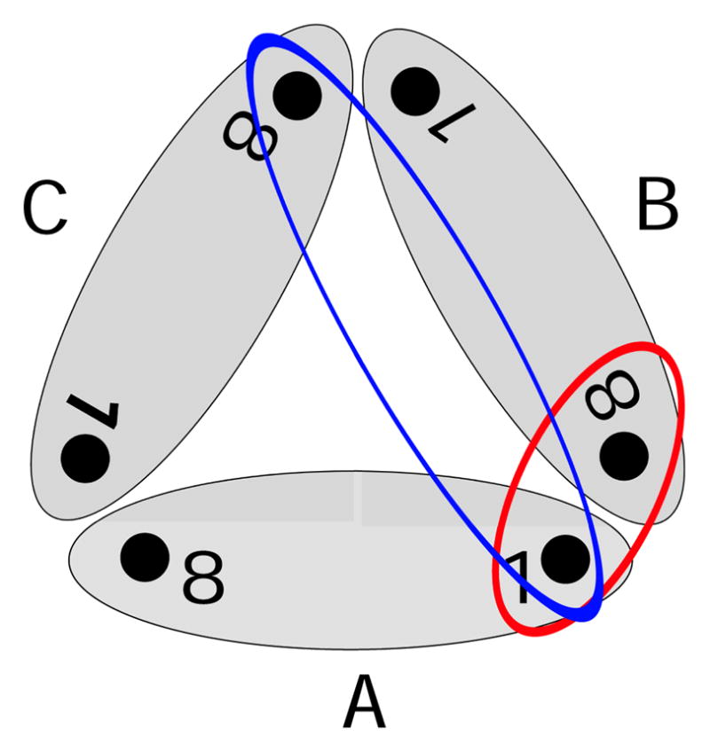
Scheme of the trimer complex and the included inter-monomer couplings: The grey ellipses represent the single monomers A–C. There are two different 1–8 couplings between different monomers. The red ellipse describes the coupling between pigment 1 and the closest BChl 8 of a neighboring monomer (also depicted as 8B). Furthermore, the blue ellipse describes the coupling between pigment 1 and the more distant pigment 8 of the third monomer. Because of symmetry there is only one 1–1 coupling.

The average values for the inter-monomer couplings extracted along the MD trajectory are given in Table 4 for the two different types of inter-monomer couplings indicated in Figure 5. The same quantities based on the crystal structure are given in Table 5. Only the mentioned inter-monomer coupling between BChl 1 and BChl 8 is larger than 2 meV. Solely one of the coupling between pigments, namely, between 7 and 8, has an average value slightly above 1 meV. All other couplings have absolute average values below 1 meV but there are many of them. As a result, excitations from one monomer will eventually “leak” to the other monomers if not removed from the system beforehand.

Table 4.

Intermonomer couplings averaged over the MD trajectory in units of meV. Upper triangle: couplings of monomer pairs of A–B, B–C and C–A. Lower triangle: couplings of monomer pairs of A–C, B–A and C–B.

	1	2	3	4	5	6	7	8
1	0.12	0.04	−0.07	0.08	0.29	0.19	0.11	2.60
2	0.18	−0.05	−0.31	−0.19	0.92	0.65	0.18	0.41
3	0.17	0.01	−0.33	0.70	0.57	0.28	0.49	0.09
4	0.04	0.06	0.08	0.24	−0.07	−0.05	0.24	−0.15
5	0.08	0.11	0.13	−0.01	0.22	0.01	−0.08	0.35
6	0.01	0.09	0.10	0.17	−0.17	−0.18	0.20	−0.90
7	0.04	0.03	−0.09	0.60	−0.20	0.01	0.71	−1.08
8	0.01	0.090	0.10	−0.10	0.16	−0.12	−0.28	0.45

Table 5.

Intermonomer couplings based on the crystal structure in units of meV. Upper triangle: couplings of monomer pairs of A–B, B–C and C–A. Lower triangle: couplings of monomer pairs of A–C, B–A and C–B.

	1	2	3	4	5	6	7	8
1	0.14	0.06	−0.06	0.08	0.31	0.16	0.13	3.17
2	0.21	−0.03	−0.32	−0.23	0.99	0.63	0.28	0.47
3	0.19	0.04	−0.28	0.63	0.61	0.27	0.58	0.08
4	0.04	0.06	0.06	0.26	−0.10	−0.04	0.26	−0.15
5	0.08	0.12	0.15	−0.04	0.24	−0.00	−0.10	0.38
6	0.00	0.09	0.09	0.19	−0.20	−0.18	0.24	−0.93
7	0.04	0.05	−0.09	0.63	−0.22	0.03	0.81	−1.08
8	0.00	0.07	0.10	−0.12	0.17	−0.13	−0.31	0.49

The coupling values stated above have all been calculated using the TrEsp approach. A very popular approximation for the coupling calculation is the point dipole approximation (PDA). Recently we tested this latter and other methods to determine coupling values for the LH2 system.²³ With 11 Å the minimum inter-pigment distance in the FMO complex is even larger than in the B800 ring. Therefore for most couplings the values calculated using the PDA are very similar to the values calculated using the TrEsp approach. The distributions (data not shown) of the couplings are, however, up to twice as broad as in the case of the PDA. Nevertheless, there are some couplings which show a significant difference. As an example we mention the coupling between pigments 5 and 6; the TrEsp method yields an average value of 6.92 meV compared to 9.17 meV obtained from the PDA. Adolphs and Renger also tabulate coupling values calculated using different approaches and based on the crystal structure. Our results for the intramonomer couplings for the crystal structure are rather similar to the values by these authors⁵³ using the transition monopole approximation with a value for the dielectric constant ε of two and the crystal structure. Actually, most of the present values are slightly smaller than those reported earlier.⁵³ As discussed above, the average couplings based on the MD simulations either for the monomer or the trimer system sometimes deviate strongly from those for the crystal structure. In all calculations below, TrEsp coupling values have been used.

Spatial correlations

As mentioned in the Introduction, spatial correlations in the fluctuations of the site energies have been suggested to underly the experimentally observed long-lived coherence of BChl excitations in FMO. In a previous publication²⁴ several of us have analyzed these correlations based on the same MD and electronic structure data as employed in the present study. Only weak atomic correlations were found. BChls 1 and 2 exhibit somewhat significant correlation in their atomic motion, but not in the fluctuation of their site energies.²⁴ Some correlation between couplings appear for cases in which two BChl pairs share a common partner. For example, there is a significant correlation between couplings 4–5 and 5–7, i.e., if pigment 5 is moving, this imposes a change in the geometric relationship between pigments 4 and 7 and, therefore, causes a correlation between the two couplings. Nevertheless, only very few couplings showed at the same time correlated fluctuations, large coupling values, and broad distributions. If one of these criteria is not fulfilled, the effect of correlated couplings is negligible. Only if two couplings are relatively large, have large fluctuations and have a non-negligible correlation, will an effect in the dynamics be observed. This is not directly visible from the correlation values since the distributions are normalized.

Transition dipole moments

The transition dipole moments (TDM) of the individual BChls determine the optical properties of the FMO complex. The direction of each BChl’s TDM is indicated in Figure 1. The dipole moment of individual BChls are often assumed to be in the direction of the N_B-N_D axis within the molecule.³⁵ In the present study the transition dipole moments have been determined through ZINDO/S calculations as detailed in Methods. The absolute values of the TDMs have been rescaled by a factor of 0.567 to a value of 6.3 Debye, when averaged over all BChls, which corresponds to the experimentally measured TDM value.⁴⁹ The relative TDM magnitudes of the individual BChls after this common rescaling are shown in the inset of Figure 6. Pigments 1–6 have similar magnitudes of their TDM, namely, 6.39 ±0.41 Debye. BChl 8 has a slightly smaller value (6.19 ±0.50 Debye) as has chromophore 7 (5.97 ±0.54 Debye). These are only averages with non-negligible fluctuations as indicated by the standard deviations. We note that there is significant deviation between the average magnitude of the transition dipole moments based on the MD simulations and the corresponding crystal structure data (also rescaled to an average value of 6.3 Debye).

Figure 6.

Magnitude and angle distributions of the TDM. The inset shows the magnitude of the transition dipole moment averaged over the trimer trajectory and the three monomers as explained in the text. The main graph shows the corresponding distribution of angles (in degrees) between the TDM and the N_B-N_D axis of the individual BChls (solid lines) together with the values based on the crystal structure (doted sticks, open squares).

In addition to the magnitude of the dipole moments, the orientation of the TDM is of importance. The deviation of the TDM direction from the N_B-N_D axis has previously been discussed. ³⁵ As can be seen in Figure 6 the values fluctuate between 0° and 10°. Concerning this property, pigments 1, 4, and 7 behave similarly. Also the pigment triple 2, 5, and 6 and the pigment pair 3 and 8 behave similarly in regard to the distribution of deviation angles. Though high precision calculations of the direction of the TDM are certainly of importance, this example shows that one should not forget in carrying out such calculations that there is quite a spread along a trajectory due to thermal fluctuation.

Supplementary to TDMs stemming from the ZINDO/S calulations, one can compute TDMs using predefined transition charges from the TrEsp approximation (see section about couplings). Compared to the distributions in Figure 6 the deviations of the directions from the N_B-N_D axis are Gaussian distributed between 0° and 5° with a peak maximum at around 2.2°(data not shown). The averaged magnitude is quite similar to that in the inset of Figure 6.

Excitation dynamics

The dynamics of the electronic properties along the room-temperature MD trajectory can be used to describe the effect of the environment on the exciton dynamics. This is sometimes called a ground-state classical path description since the MD trajectory is a ground state trajectory based on classical dynamics, i.e., it does not include the dynamics on excited electronic states. Nevertheless, this procedure is expected to yield a rather useful description for excitation energy transfer processes. For charge transfer scenarios this might be less accurate since a moving charge influences a classical MD simulation much more than a rather localized excitation. For the present purpose one may first determine the spectral density and then compute exciton dynamics and optical spectra.^23,27 Here we employ an alternative strategy and use the time-dependent site energies of the pigments and their couplings in a wave packet calculation^{40,41,55–57} employing the NISE approach. In this approach the evolution of the wavefunction is calculated by solving the time-dependent Schrödinger equation for the fluctuating Hamiltonian. As this cannot be done directly time is divided into short time intervals during which the Hamiltonian can be assumed to be constant. The time-independent Schrödinger equation is then solved successively for each time interval providing the solution of the time-dependent Schrödinger equation as long as the short time intervals are brief enough. This implies that the actual fluctuating Hamiltonian is used directly in determining the exciton dynamics and no assumptions on the nature of the spectral density or density of states is made. The averaging of the fluctuations is achieved by averaging over multiple starting configurations along the trajectory. For calculating the exciton dynamics this was done assuming that the excitation was initially localized on one of the sites. The exciton dynamics was determined using the complete trajectory length available, i.e., 300 ps for the monomer and 200 ps for the trimer simulations with 5 fs time steps between snapshots. The calculations of 1000 fs length were repeated with starting times 100 fs apart in order to average over sufficient starting configurations of the bath. This sample rate is chosen because temporal correlation of the individual site energies is negligible after 50 fs.

Before analyzing the population dynamics in the FMO complex we want to emphasize once more that the present calculations are based on room-temperature MD simulations. Many previous results for the excitation dynamics in the FMO complex are based on model assumptions for a spectral density and often have been performed at 77 K.^{15–19,21,22,25} This lower temperature in previous studies lead to less dephasing in the excitation dynamics compared to the one shown below. To illustrate the resulting population dynamics we excited individual pigments in the FMO monomer. In Figure 7 the corresponding population decay is shown for the initially excited chromophore. In case that BChl 1 is excited, 50 % of the excitation remains at this pigment for 1000 fs while for BChl 4 it remains there only for 100 fs. The time difference agrees with the coupling values resulting from the monomer simulation as seen in Figure 4. The coupling to pigment 1 is small while the largest coupling is found to chromophore 4. Interestingly, the situation changes when performing the same kind of simulations for the trimer, as shown in Figure 8. Of course, in case of the trimer simulations there are three different population decays for initially exciting a specific pigment in one of the three monomers. The three respective curves are seen to be similar but not identical. With sufficient sampling, these curves should become identical. In the trimer case the population transfer away from the initially excited pigments 1 or 2 is much faster than in case of the monomer simulations. As can be seen in Figure 8 and discussed above, the coupling between BChl 1 and 2 is lower by a factor of 2.5 in the monomer case leading to slower population transfer from the initially excited BChl 1 to BChl 2 in the same monomer and vice versa. Furthermore, one single coherent oscillation is observed in the population transfer from BChl 1. Initially exciting BChl 8 leads to the slowest transfer to the other pigments. Transfer from the other chromophores proceeds at similar speed in the cases of monomer and trimer. The difference between monomer and trimer simulations is partly due to the different long-time limits imposed by the theory. The wave packet simulations employed here implicitly include a high-temperature limit, i.e., in the thermodynamics limit all sites are equally populated. Since the number of sites in the monomer and trimer case are different in the different simulations, also the long-time populations of the two different simulations are not the same.

Figure 7.

Population dynamics based on the monomer simulation. Shown is the population decay from the respective initially excited chromophore in a monomer, i.e., the decay shown results from calculations with seven different initial conditions.

Figure 8.

Same as in Figure 7 based on the trimer simulation. The line style distinguishes the three monomers.

In vivo, the FMO complex is supposed to transfer excitation energy from the chlorosomes to the reaction center. This motivates one to take a closer look at energy transfer in this direction. In Figure 9 the population transfer from site 1 to site 3 is shown, i.e., in the simulation site 1 was initially excited and the population increase at site 3 was monitored. The same is shown for the transfer from site 6 to 4. The population transfer is fitted with a function assuming direct transfer between the pairs: P(t) = A(1 − exp(−t/T₁)). The transfer times T₁ for the transfer between site 1 and 3 is 58 fs and between 4 and 6 is 29 fs. The deviation in the initial parts of the fit is due to the actual involvement of intermediate steps. The long-time decay observed for the 6 to 4 transfer arises because the population is first transferred quickly between those sites and only slowly to other sites in the complex. If one knows the number of intermediate steps the transfer can be treated using Poisson statistics.⁵⁸ Instead of attempting to construct a complex model for the transfer, we will here simply make the observation that the transfer across several BChls within the FMO complex and involving BChls 1 to 7 is predicted to be very quick within our model with transfer times below 100 fs. Though BChl 7 has the largest average energy, it is nevertheless involved in some of the energy transfer pathways. Initially exciting BChl 6, for example, leads to roughly the same excitation on chromophores 5, 6, and 7 after 1 ps. In case BChl 1 is initially excited, basically no excitation energy goes through BChl 7.

Figure 9.

Population transfer across the FMO complex trimer over the three monomers. Shown as solid line is the increase of population on sites 3 and 4, respectively. The dashed lines indicate the corresponding fits. BChls 8′ and 8″ belong to neighbouring monomers.

In addition to the intra-monomer dynamics discussed, transfer from BChl 8 of the three different monomers to BChl 3 in a specific monomer is displayed in Figure 9. The fastest transfer between BChls 8 and 3 does not take place within one monomer, but between different monomers with a transfer time T₁ of about 1.4 ps. As mentioned above, the coupling of this pigment to the other BChls in the same monomer is smaller than that to one of the other two neighbouring monomers. This is due to the spatial organisation of the BChls in the FMO complex as already indicated in Figure 1. Inter-monomer transfer is mainly due to BChl 8; transfer away from BChl 8 in Figure 8 is mainly caused by transfer to a neighboring monomer.

Spectroscopy

Linear absorption and two-dimensional spectra were calculated for the FMO trimer using the NISE approach,⁴¹ describing the exciton dynamics in the same way as in the previous section. To calculate the response functions governing the linear and two-dimensional spectra we employed a recently developed sparse matrix algorithm⁴⁵ including the split operator propagation scheme for propagating two-exciton states.⁵⁹ This sparse scheme was only applied during the coherence times (t₁ and t₃), while the exact one-exciton Hamiltonian was propagated during the waiting time (t₂). This scheme was developed for treating coupled three level systems, i.e., systems where two-exciton states with double excitation on the same site are also allowed. Here, this third level was effectively eliminated by adding a large artificial anharmonicity moving the third level far away from the off-site two-eciton states.⁶⁰ The spectra were calculated for 100 ps of the trimer trajectory with 5 fs between the snapshots and for the full 300 ps of the monomer trajectory. The spectral calculation was repeated with starting times 50 fs apart resulting in a total of 1975 samples for the two-dimensional spectra for the trimer. In case of the monomer the calculation was repeated 100 fs apart resulting in a total of 2988 samples. For the linear absorption the sample times were 5 fs apart resulting in a total of 19360 samples for the trimer and 59744 samples for the monomer. The coherence times were sampled using 5 fs intervals up to 640 fs for both monomer and trimer. Furthermore, the waiting time was probed with 25 fs intervals up to 1000 fs. Orientational averaging was performed by averaging over the 21 unique molecular frame polarization directions and adding those up with the proper weight factors to obtain the parallel and perpendicular polarization spectra.⁶¹ Finally, the 2D CS spectra were obtained by a double Fourier transform of the coherence times into the two frequency axes ω₁ and ω₃.

In Figure 10 the linear absorption spectra are shown. The monomer as well as the trimer spectra contain one peak with a long tail stretching to higher frequencies. In both cases the position of this peak is at 12020 cm⁻¹ (1.49 eV), i.e., close to the typical position of the single site energies (see Figure 2). The overall peak shape also resembles the single site DOS. The full-width-half-maximum (FWHM) of the absorption peak is 320 cm⁻¹ (40 meV) for the trimer and 391 cm⁻¹ (49 meV) for the monomer. For the FMO complex of Chlorobaculum tepidum the linear absorption at room temperature was measured by Freiberg et al.⁶² The experimental absorption peak is at 12350 cm⁻¹ (1.53 eV) and the FWHM of the spectrum is 448 cm⁻¹ (56 meV). As in the calculated spectrum a tail stretching to higher frequencies is observed, which indicates that the non-Gaussian site energy distribution that we find is real. To obtain the same peak position for both, the simulated and the experimental spectra, one could introduce a common shift for all site energies of 42 meV as discussed above. Both the simulated and the experimental widths are smaller than the typical width of the DOS of about 525 cm⁻¹ (62 meV). This means that the spectrum is narrowed due to exchange and motional narrowing effects. To analyze this in more detail we calculated the spectra in the static limit, where the effect of motional narrowing is neglected. We found that the linear spectra are comparable in width to the DOS, leading to the conclusion that the narrowing of the spectrum is due to fast fluctuations of the site energies. This is further supported by the observation that the delocalization length according to the definition of Thouless⁶³ is only 1.4 for the monomer and 1.6 for the trimer indicating that the excitations are predominantly localized.

Figure 10.

Linear absorption spectrum for FMO at room temperature calculated for the trimer (black solid line) and monomer (red solid line) along with the experimental data for the monomer (dashed line) extracted from Freiberg et al.⁶²

The bandwidth in the discussed spectra is about 60 meV, which corresponds to k_BT for a temperature of 700 K. This value implies that one needs to be concerned with finite temperature effects. For the linear spectra temperature effects should not be significant, however, since the spectral dephasing time (~30 fs) is shorter than the population transfer times. As stated in Introduction, previous simulations of the exciton transfer for the OH-stretch vibration, where the bandwidth is about 2 k_BT, ⁴⁵ found good agreement with experiment.

The 2D CS spectra with parallel polarization of the monomer and trimer are shown in Figure 11 and Figure 12 for a representative subset of waiting times. Since no excited state absorption can be recognized, only one peak is observed, originating from ground state bleach and stimulated emission. Experimentally such peak was detected (also for Chlorobaculum tepidum) above the main peak at lower temperatures.¹¹ The excited state absorption decreases in experiment with increasing temperature and is almost gone at 277 K. The magnitude and position of the ground state bleach and stimulated emission peak is a signature of strong exitonic coupling and delocalization.^26,64 The present spectra thus demonstrate that excitations at 300 K are predominantly localized, in agreement with the delocalization length discussed previously. For the linear absorption, the peak position in the calculated 2D CS spectra is at lower energies than in the experiment¹¹ and the line width is a bit narrower. It is noteworthy that the trimer spectrum is narrower than the monomer spectrum demonstrating that the trimer is more ordered. Comparing the shape obtained for the monomer in a 300 K simulation for a waiting time of 400 fs with that observed at the same waiting time but at 277 K, the calculated spectrum has more pronounced wings, which is typical for faster site energy fluctuations. The difference might simply arise since the higher temperature in the simulation results in faster fluctuations or it can be an indication that the fluctuations caused by the dynamics in our molecular dynamics simulations are too fast.

Figure 11.

The 2D correlation spectroscopy spectrum with parallel polarization and different waiting times of the monomer. To amplify weak features, the contours are plotted at equidistant (10%) intervals of arcsinh(10×S), where S is the signal normalized to the peak height for waiting time zero.

Figure 12.

The 2D correlation spectroscopy spectrum with parallel polarization and different waiting times for the trimer. The contours are plotted as in Figure 11.

We extracted the frequency integrated anisotropy from the 2D CS spectra as shown in Figure 13. This anisotropy is a frequently used measure of the orientational motion or population transfer.^41,65 For the extraction, we fitted the anisotropy to a biexponential function with offset. For the monomer we found decay constants 55 fs and 240 fs, and for the trimer we found 50 fs and 420 fs. Apart from a bump at 300 fs for the trimer and at 600 fs for the monomer with heights of these bumps smaller than the error bars in the simulation results, there is no indication of coherent oscillations. The obtained time scales compare well with the time scales typically found in population transfer analysis. The anisotropy decay is completely attributed to exciton transfer between different sites, since the BChls are not reorienting significantly on the sub-picosecond time scale. This attribution is also supported by calculating the anisotropy from the autocorrelation of the TDM as given by equation 9 in Ref. 66. For the trimer the anisotropy decays to below 0.1 within a picosecond, indicating that the average excitation at this time is delocalized over more than two units. If only two units are involved the anisotropy cannot decay below 0.1, unless the molecules rotate into the third dimension not spanned by their initial transition dipole moment vectors. In contrast, the monomer anisotropy never decays below 0.1. The faster decay in the trimer is a direct reflection of the fact that the population dynamics is faster than in the monomer.

Figure 13.

Calculated polarization anisotropy of the peak in the 2D correlation spectroscopy spectra at different waiting times for monomer (red, solid line) and trimer (black, solid line), along with biexponential fits (dotted lines). In addition, the calculated anisotropy from the autocorrelation of the transition dipole moments (dashed lines) is shown.

The diagonal peak intensity for the parallel and perpendicular polarization directions is given in Figure 14. The intensities were extracted near the peak maximum at ω₁/2πc = ω₃/2πc =12000 cm⁻¹. The peak for the parallel polarization is particularly sensitive to population transfer. The anisotropy in the perpendicular polarization spectra remains constant on the time scale shown, while the anisotropy in the parallel polarization spectra exhibit biexponential decays similar to those observed in the anisotropy decay. Neither of the peaks exhibit signatures of coherent oscillations.

Figure 14.

The diagonal peak intensity of the 2D correlation spectroscopy spectra at different waiting times for the monomer (red) and the trimer (black). The solid lines are biexponential fits with an offset.

Finally, we extracted the absolute value of the off-diagonal intensity taken 150 cm⁻¹ below the peak (see Figure 15). This particular point is chosen for comparing with the off-diagonal point examined by Engel et al.¹¹ At this point no cross peak is resolved at room temperature, but a hidden cross peak between two BChl a chromophores might affect the spectrum. For the parallel polarization no oscillations can be resolved. The decay behavior is again typical for population transfer. For the perpendicular polarization a weak damped oscillation is observed. The oscillation is slightly larger for the trimer, but longer lived for the monomer. Attempts to fit the oscillations reveal that the dominant frequency is 136 cm⁻¹ in both cases. In particular for the monomer it is, however, difficult to obtain a unique fit and due to the level of noise we refrain from attributing significance to the oscillations. We do, however, note that the dominant frequency coincides with the 160 cm⁻¹ frequency experimentally observed at lower temperature.¹¹

Figure 15.

The absolute value of the off-diagonal peak intensity of the 2D correlation spectroscopy spectra at different waiting times. Taken at ω₁/2πc=12000 cm⁻¹ and ω₃/2πc=11850 cm⁻¹. The monomer data is given in red and the trimer data in black. The full lines are fits.

Conclusions

In this study we have performed simulations of the exciton dynamics and optical spectra for the FMO complex starting from MD simulations and employing quantum chemistry calculations to generate a time-dependent exciton Hamiltonian. Simulations were performed for both a single FMO monomer and a trimer. Interestingly, in the monomer simulations, an eighth BChl, only recently found in a new crystal structure, did not form a stable complex with the rest of the protein. The main monomer simulations were therefore carried out with only seven BChls. The MD trajectories at room temperature show the thermal fluctuations of the atoms within the protein and the BChl molecules.

In subsequent semi-empirical quantum chemical calculations along the MD trajectory, the effect of thermal fluctuations on ground and first excited state of the BChl molecules was calculated. We found that the gaps between first excited state and ground state, denoted as site energies, show similarities and differences with previous studies. The distributions of calculated site energies show rather broad non-Gaussian fluctuations which are much broader than the splitting between individual site energies; the distributions also exhibit pronounced blue tails. The distribution widths of the intra-monomer and inter-monomer BChl couplings are roughly proportional to the absolute value of the couplings. In a previous study we already showed that at ambient temperatures no relevant spatial correlation could be found in the site energies or the couplings.²⁴

Based on the results from the electronic structure calculations, we were able to parametrize a time-dependent model of coupled sites. The solution of the Schrödinger equation in this model revealed the excitation energy transfer within the FMO complex as well as optical properties. Due to the different coupling values in the monomer and trimer results, especially between BChls 1 and 2, the exciton dynamics based on monomer and trimer MD simulations were found to differ significantly. Within the trimer the coupling between the pigments 1 and 2 is so large that faint coherent oscillations are observed despite the fluctuating environment. This observation may be connected to the experimentally observed coherences at room temperature.¹¹ In general the population transfer between different states was faster in the trimer due to larger couplings and narrower site energy distributions. One can therefore expect coherent oscillations to be larger in the trimer than those already observed in the monomer.

Transfer between individual chromophores, whether directly or indirectly connected by strong couplings, occurs on time scales below 100 fs. Interestingly, although the 8th BChl is situated closest to the chlorosome baseplate,⁶⁷ indicating that it could be the first pigment to receive excitation from the chlorosome, it has the slowest transfer rate to any other pigment. The role of 8th BChl may thus only be to assist excitation transfer between FMO monomers within the trimer and not to directly receive excitation from the chlorosome.

Optical properties of the FMO monomer and trimer complex were determined. For the monomer the simulated peak position of the linear absorption is only about 3% off the experimental value and the width is 15% narrower than the observed width. The skewed shape of the experimental absorption line shape is well reproduced by the simulation. The skewness originates from the non-Gaussian distribution of the individual site energies. The overly narrow line width may be a result in the simulations from inaccuracies in the force field parameters, use of ground-state classical path dynamics, undersampling of protein conformations, neglect of polarization effects, low sensitivity to fluctuations in the environment, errors in site energies based on the semi-empirical ZINDO/S method or too fast environmental fluctuations resulting in too much exchange narrowing. Furthermore, the TrEsp couplings are based on fixed transition charges and have been mapped onto dynamical structures which might also change the effect of exchange narrowing. On the positive side we note that the calculated 2D CS spectra show no distinct features just as in the experimental counterparts at 277 K. In the absolute value of the off-diagonal intensity taken 150 cm⁻¹ below the peak, very small oscillations are visible, which might be connected to what is seen in experiment at lower temperatures. To establish a clearer connection one would have to repeat simulations at lower temperatures. Here we considered the energy transfer through the FMO complex at room temperature. At lower temperatures the transfer mechanism is surely different as the magnitude and speed of the dynamics of the environmental will be smaller and slower.

From our simulations we find that even though little coherent population transfer between sites is observed in the FMO complex at room temperature the overall excitation transfer is very efficient with transfer times across the complex of only 100 fs. The transfer is predominantly occurring through the individual monomers which can be thought of as individual energy transfer channels due to small couplings between sites in different monomers. The transfer is more efficient in the naturally ocuring trimer than in the monomer due to smaller energy fluctuations and larger couplings. The reason that the transfer, even though incoherent, can be highly efficient is that the site energy fluctuations are very fast, resulting in non-adiabatic population transfer occurring every time the site energies of coupled sites are close, which happens on a 100 fs time scale.

References

- 1.Hu X, Ritz T, Damjanović A, Autenrieth F, Schulten KQ. Rev Biophys. 2002;35:1–62. doi: 10.1017/s0033583501003754. [DOI] [PubMed] [Google Scholar]
- 2.Cogdell RJ, Gall A, Köhler J. Q Rev Biophys. 2006;39:227–324. doi: 10.1017/S0033583506004434. [DOI] [PubMed] [Google Scholar]
- 3.Cheng YC, Fleming GR. Annu Rev Phys Chem. 2009;60:241–242. doi: 10.1146/annurev.physchem.040808.090259. [DOI] [PubMed] [Google Scholar]
- 4.Novoderezhkin VI, van Grondelle R. Phys Chem Chem Phys. 2010;12:7352–7365. doi: 10.1039/c003025b. [DOI] [PubMed] [Google Scholar]
- 5.Milder MT, Brüggemann B, van Grondelle R, Herek JL. Photosynth Res. 2010;104:257–264. doi: 10.1007/s11120-010-9540-1. [DOI] [PMC free article] [PubMed] [Google Scholar]
- 6.Matthews BW, Fenna RE, Bolognesi MC, Schmid MF, Olson JM. J Mol Biol. 1979;131:259–265. doi: 10.1016/0022-2836(79)90076-7. [DOI] [PubMed] [Google Scholar]
- 7.Tronrud DE, Schmid MF, Matthews BW. J Mol Biol. 1986;188:443–444. doi: 10.1016/0022-2836(86)90167-1. [DOI] [PubMed] [Google Scholar]
- 8.Tronrud DE, Wen J, Gay L, Blankenship RE. Photosynth Res. 2009;100:79–87. doi: 10.1007/s11120-009-9430-6. [DOI] [PubMed] [Google Scholar]
- 9.Brixner T, Stenger J, Vaswani HM, Cho M, Blankenship RE, Fleming GR. Nature. 2005;434:625–628. doi: 10.1038/nature03429. [DOI] [PubMed] [Google Scholar]
- 10.Engel GS, Calhoun TR, Read EL, Ahn TK, Mancal T, Cheng YC, Blankenship RE, Fleming GR. Nature. 2007;446:782–786. doi: 10.1038/nature05678. [DOI] [PubMed] [Google Scholar]
- 11.Panitchayangkoon G, Hayes D, Fransted KA, Caram JR, Harel E, Wen J, Blankenship RE, Engel GS. Proc Natl Acad Sci USA. 2010;107:12766–12770. doi: 10.1073/pnas.1005484107. [DOI] [PMC free article] [PubMed] [Google Scholar]
- 12.Collini E, Wong CY, Wilk KE, Curmi PM, Brumer P, Scholes GD. Nature. 2010;463:644–647. doi: 10.1038/nature08811. [DOI] [PubMed] [Google Scholar]
- 13.Collini E, Scholes GD. Science. 2009;323:369–373. doi: 10.1126/science.1164016. [DOI] [PubMed] [Google Scholar]
- 14.Wolynes PG. Proc Natl Acad Sci USA. 2009;106:17247–17248. doi: 10.1073/pnas.0909421106. [DOI] [PMC free article] [PubMed] [Google Scholar]
- 15.Caruso F, Chin AW, Datta A, Huelga SF, Plenio MB. J Chem Phys. 2009;131:105106. [Google Scholar]
- 16.Rebentrost P, Mohseni M, Aspuru-Guzik A. J Phys Chem B. 2009;113:9942–9947. doi: 10.1021/jp901724d. [DOI] [PubMed] [Google Scholar]
- 17.Nazir A. Phys Rev Lett. 2009;103:146404. doi: 10.1103/PhysRevLett.103.146404. [DOI] [PubMed] [Google Scholar]
- 18.Fassioli F, Nazir A, Olaya-Castro A. J Phys Chem Lett. 2010;1:2139–2143. [Google Scholar]
- 19.Nalbach P, Eckel J, Thorwart M. New J Phys. 2010;12:065043. [Google Scholar]
- 20.Strümpfer J, Schulten K. J Chem Phys. 2011;134:095102. doi: 10.1063/1.3557042. [DOI] [PMC free article] [PubMed] [Google Scholar]
- 21.Fleming GR, Huelga S, Plenio M. New J Phys. 2010;12:065002. [Google Scholar]
- 22.Abramavicius D, Mukamel S. J Chem Phys. 2011;134:174504. doi: 10.1063/1.3579455. [DOI] [PMC free article] [PubMed] [Google Scholar]
- 23.Olbrich C, Kleinekathöfer U. J Phys Chem B. 2010;114:12427–12437. doi: 10.1021/jp106542v. [DOI] [PubMed] [Google Scholar]
- 24.Olbrich C, Strümpfer J, Schulten K, Kleinekathöfer U. J Phys Chem B. 2011;115:758–764. doi: 10.1021/jp1099514. [DOI] [PMC free article] [PubMed] [Google Scholar]
- 25.Abramavicius D, Mukamel S. J Chem Phys. 2010;133:064510. doi: 10.1063/1.3458824. [DOI] [PubMed] [Google Scholar]
- 26.Dijkstra AG, Jansen TLC, Knoester J. J Chem Phys. 2008;128:164511. doi: 10.1063/1.2897753. [DOI] [PubMed] [Google Scholar]
- 27.Damjanović A, Kosztin I, Kleinekathöfer U, Schulten K. Phys Rev E. 2002;65:031919. doi: 10.1103/PhysRevE.65.031919. [DOI] [PubMed] [Google Scholar]
- 28.Walker RC, Mercer IP, Gould IR, Klug DR. J Comput Chem. 2007;28:478–480. doi: 10.1002/jcc.20559. [DOI] [PubMed] [Google Scholar]
- 29.Zwier MC, Shorb JM, Krueger BP. J Comput Chem. 2007;28:1572–1581. doi: 10.1002/jcc.20662. [DOI] [PubMed] [Google Scholar]
- 30.Janosi L, Kosztin I, Damjanović A. J Chem Phys. 2006;125:014903. doi: 10.1063/1.2210481. [DOI] [PubMed] [Google Scholar]
- 31.Olbrich C, Liebers J, Kleinekathöfer U. phys stat sol (b) 2011;248:393–398. [Google Scholar]
- 32.Ridley J, Zerner MC. Theor Chim Acta. 1973;32:111–134. [Google Scholar]
- 33.Linnanto J, Korppi-Tommola J. Phys Chem Chem Phys. 2006;8:663–667. doi: 10.1039/b513086g. [DOI] [PubMed] [Google Scholar]
- 34.Madjet ME, Abdurahman A, Renger T. J Phys Chem B. 2006;110:17268–81. doi: 10.1021/jp0615398. [DOI] [PubMed] [Google Scholar]
- 35.Renger T. Photosynth Res. 2009;102:471–485. doi: 10.1007/s11120-009-9472-9. [DOI] [PubMed] [Google Scholar]
- 36.Madjet ME, Müh F, Renger T. J Phys Chem B. 2009;113:12603–14. doi: 10.1021/jp906009j. [DOI] [PubMed] [Google Scholar]
- 37.de Boeij WP, Pshenichnikov MS, Wiersma DA. Chem Phys Lett. 1996;253:53. doi: 10.1103/PhysRevLett.76.4701. [DOI] [PubMed] [Google Scholar]
- 38.Hamm P, Lim MH, Hochstrasser RM. J Phys Chem B. 1998;102:6123. [Google Scholar]
- 39.Ernst RR, Bodenhausen G, Wokaun A. Principles of nuclear magnetic resonance in one and two dimensions. Oxford University Press; New York: 1995. [Google Scholar]
- 40.Jansen TLC, Knoester J. J Phys Chem B. 2006;110:22910–22916. doi: 10.1021/jp064795t. [DOI] [PubMed] [Google Scholar]
- 41.Jansen TLC, Knoester J. Acc Chem Res. 2009;42:1405–1411. doi: 10.1021/ar900025a. [DOI] [PubMed] [Google Scholar]
- 42.Ishizaki A, Fleming GR. J Chem Phys. 2009;130:234111. doi: 10.1063/1.3155372. [DOI] [PubMed] [Google Scholar]
- 43.Sharp LZ, Egorova D, Domcke W. J Chem Phys. 2010;132:014501. doi: 10.1063/1.3268705. [DOI] [PubMed] [Google Scholar]
- 44.Palmieri B, Abramavicius D, Mukamel S. Phys Chem Chem Phys. 2010;12:108–114. doi: 10.1039/b916723d. [DOI] [PubMed] [Google Scholar]
- 45.Jansen TLC, Auer BM, Yang M, Skinner JL. J Chem Phys. 2010;132:224503. doi: 10.1063/1.3454733. [DOI] [PubMed] [Google Scholar]
- 46.Humphrey WF, Dalke A, Schulten K. J Mol Graph. 1996;14:33–38. doi: 10.1016/0263-7855(96)00018-5. [DOI] [PubMed] [Google Scholar]
- 47.Petrenko T, Neese F. J Chem Phys. 2007;127:164319. doi: 10.1063/1.2770706. [DOI] [PubMed] [Google Scholar]
- 48.Cory MG, Zerner MC, Hu X, Schulten K. J Phys Chem B. 1998;102:7640–7650. [Google Scholar]
- 49.Alden RG, Johnson E, Nagarajan V, Law WWPJ, Cogdell RG. J Phys Chem B. 1997;101:4667–4680. [Google Scholar]
- 50.Scholes GD, Curutchet C, Mennucci B, Cammi R, Tomasi J. J Phys Chem B. 2007;111:6978–6982. doi: 10.1021/jp072540p. [DOI] [PubMed] [Google Scholar]
- 51.Vulto SIE, de Baat MA, Louwe RJW, Permentier HP, Neef T, Miller M, van Amerongen H, Aartsma TJ. J Phys Chem B. 1998;102:9577–9582. [Google Scholar]
- 52.Renger T, May V. J Phys Chem A. 1998;102:4381–4391. [Google Scholar]
- 53.Adolphs J, Renger T. Biophys J. 2006;91:2778–2787. doi: 10.1529/biophysj.105.079483. [DOI] [PMC free article] [PubMed] [Google Scholar]
- 54.Schmidtam Busch M, Müh F, Madjet ME, Renger T. J Phys Chem Lett. 2011;2:93–98. doi: 10.1021/jz101541b. [DOI] [PubMed] [Google Scholar]
- 55.Kobus M, Gorbunov RD, Nguyen P, Stock G. Chem Phys. 2008;347:208–217. [Google Scholar]
- 56.Zhu H, May V, Röder B, Renger T. J Chem Phys. 2008;128:154905. doi: 10.1063/1.2890721. [DOI] [PubMed] [Google Scholar]
- 57.Zhu H, Röder B, May V. Chem Phys. 2009;362:19–26. [Google Scholar]
- 58.Deranleau DA. Experientia. 1982;38:661–662. doi: 10.1007/BF01964078. [DOI] [PubMed] [Google Scholar]
- 59.Paarmann A, Hayashi T, Mukamel S, Miller RJD. J Chem Phys. 2009;130:204110. doi: 10.1063/1.3139003. [DOI] [PMC free article] [PubMed] [Google Scholar]
- 60.Abramavicius D, Palmieri B, Voronine DV, Sanda F, Mukamel S. Chem Rev. 2009;109:2350–2358. doi: 10.1021/cr800268n. [DOI] [PMC free article] [PubMed] [Google Scholar]
- 61.Hochstrasser RM. Chem Phys. 2001;266:273–284. [Google Scholar]
- 62.Freiberg A, Lin S, Timpmann K, Blankenship RE. J Phys Chem B. 1997;101:7211–7220. doi: 10.1021/jp9633761. [DOI] [PubMed] [Google Scholar]
- 63.Thouless DJ. Phys Rep. 1974;13:93. [Google Scholar]
- 64.Bakalis LD, Knoester J. J Phys Chem B. 1999;103:6620–6628. [Google Scholar]
- 65.Woutersen S, Bakker HJ. Nature. 1999;402:507. [Google Scholar]
- 66.Lin Y-S, Pieniazek PA, Yang M, Skinner JL. J Chem Phys. 2010;132:174505. doi: 10.1063/1.3409561. [DOI] [PubMed] [Google Scholar]
- 67.Wen J, Zhang H, Gross ML, Blankenship RE. Proc Natl Acad Sci USA. 2009;106:6134–6139. doi: 10.1073/pnas.0901691106. [DOI] [PMC free article] [PubMed] [Google Scholar]