Power and instrument strength requirements for Mendelian randomization studies using multiple genetic variants

Abstract

Background Mendelian Randomization (MR) studies assess the causality of an exposure–disease association using genetic determinants [i.e. instrumental variables (IVs)] of the exposure. Power and IV strength requirements for MR studies using multiple genetic variants have not been explored.

Methods We simulated cohort data sets consisting of a normally distributed disease trait, a normally distributed exposure, which affects this trait and a biallelic genetic variant that affects the exposure. We estimated power to detect an effect of exposure on disease for varying allele frequencies, effect sizes and samples sizes (using two-stage least squares regression on 10 000 data sets—Stage 1 is a regression of exposure on the variant. Stage 2 is a regression of disease on the fitted exposure). Similar analyses were conducted using multiple genetic variants (5, 10, 20) as independent or combined IVs. We assessed IV strength using the first-stage F statistic.

Results Simulations of realistic scenarios indicate that MR studies will require large (n > 1000), often very large (n > 10 000), sample sizes. In many cases, so-called ‘weak IV’ problems arise when using multiple variants as independent IVs (even with as few as five), resulting in biased effect estimates. Combining genetic factors into fewer IVs results in modest power decreases, but alleviates weak IV problems. Ideal methods for combining genetic factors depend upon knowledge of the genetic architecture underlying the exposure.

Conclusions The feasibility of well-powered, unbiased MR studies will depend upon the amount of variance in the exposure that can be explained by known genetic factors and the ‘strength’ of the IV set derived from these genetic factors.

Introduction

Mendelian Randomization (MR) is a method used to test or estimate a causal effect of an exposure on a disease outcome when the exposure has a known genetic determinant.^1,2 Data on such a genetic determinant, also known as an instrumental variable (IV), can be analysed jointly with exposure and outcome data to determine if an observed exposure–disease association is causal. Typically, MR is utilized when an observed exposure–outcome association is potentially attributable, at least in part, to confounding or reverse causation. In the absence of these phenomena, simple measures of association provide more precise effect estimates.

A valid MR analysis requires that the IV is (i) associated with the exposure, (ii) independent of the outcome given the exposure and confounders of the exposure–outcome association and (iii) independent of factors that confound the exposure–outcome relationship. Because genetic variation is randomly assigned prior to conception, it is not expected to be affected by any confounding factors other than ancestry, which can be accurately measured and accounted for using genetic data.³ Consequently, if the IV affects the outcome only through the exposure, the unconfounded effect of the exposure on the outcome can be captured by comparing the effect of the IV on exposure to the indirect effect of the IV on the outcome. IV analysis is common in the econometrics literature,⁴ although MR is a specific type of IV analysis in which is the IVs are genetic variants.

MR studies are becoming more feasible, as recent genome wide association (GWA) studies have identified genetic determinants (typically single nucleotide polymorphisms) for many health-related biomarkers. For example, GWA studies have linked high-density lipoprotein to 11 loci, low-density lipoprotein to 14 loci and triglycerides to 11 loci.^5–7 Genetic determinants have also been identified for C-reactive protein;^8,9 plasma levels of vitamins B,^10,11 A¹² and E;¹² mean platelet volume;^13,14 blood pressure^15,16 and fasting plasma glucose.^17–20 Several recent publications highlight the potential for GWA studies of many biomarkers simultaneously.^21–24 Such parallel GWA studies could expand our knowledge of biomarker-related polymorphisms very quickly, and as our understanding of these polymorphisms’ functions improve, the broad application of MR methodology to epidemiological and biomarker research may become feasible.

In light of these developments, we have conducted a simulation study evaluating power and IV strength requirements for MR analyses using two-stage least squares (2SLS) regression, the most common statistical method used in MR studies of continuous exposures and continuous outcomes.^25,26 We provide power calculations for IVs of varying strength and exposures of varying effect, under realistic scenarios given current knowledge. We explore the use of multiple genetic variants in MR studies, employing different strategies to combine information across variants and evaluating the consequences of these strategies on power and overall IV strength, as measured by the first-stage F statistic in 2SLS. Weak IVs lead to biased effect estimates in the presence of confounding of the exposure–outcome relationship.^27–30 We intend for this work to guide researchers in their design of future MR studies, in selecting appropriate genetic variants, constructing strong IVs and obtaining adequate sample sizes.

Methods

Power estimates were generated using simulated data sets of samples drawn from a genetically homogenous population. Each simulation consisted of 10 000 data sets containing one or more biallelic loci (G) in Hardy–Weinberg equilibrium, a continuous exposure (X) affected by G and a continuous outcome (Y) affected positively by X. Each power estimate was obtained by applying 2SLS to all 10 000 simulated data sets and determining the percentage of data sets in which a positive effect of the fitted X on Y was observed using a two-sided significance test (α = 0.05). The effect estimate from each simulated data set was also retained. Stage 1 of the 2SLS is a regression of the X on the IV(s) (G). Stage 2 is a regression of Y on the fitted X-values from Stage 1. In other words, only the variation in X that is explained by the IV(s) is used in Stage 2.

We extract two key parameters from each Stage 1 regression: R² and the F statistic. R² is the proportion of variability in the X that is explained by G, an indicator of power for MR studies. F reflects the ‘strength’ of an IV or a set of IVs. In the presence of X–Y confounding, 2SLS effect estimates will be biased towards the confounded X–Y association, but the size of the relative bias is inversely related to F (‘relative bias’ is defined as the ratio of the 2SLS bias to the bias of the confounded X–Y association).^29,30 In the MR literature, a threshold of F < 10 has typically been used to define a ‘weak IV’ (the Staiger–Stock rule³¹). This rule of thumb is based on the observation that an F value greater than ~11 ensures that relative bias will be <10% at least 95% of the time, regardless of the number of IVs used in the analysis.²⁹ The F statistic is defined as the ratio of the mean square of the model to the mean square of the error. However, F can be expressed as a function of the first-stage R², the sample size (n) and the number of IVs (k):

(1)

Thus, F increases as R² and n increase, but F decreases as k increases. We also extract the ‘adjusted R²’ from each 2SLS regression, a modification of R² that adjusts for inflation due to large numbers of predictors and small sample sizes.³² The adjusted R² is defined as:

(2)

Thus, for a given R², the adjusted R² decreases as the number of IVs (k) increases and approaches R² as the sample size increases. For simulations in which the R² and/or the adjusted R² were held constant, the appropriate effect sizes were found using an iterative search process.

Data simulation 1: Power estimates for MR studies using one genetic variant

Each simulated data set consisted of Y, X and a single G as an IV, both with and without an unobserved confounding variable, U (Figure 1a). The genotype at G was randomly generated, assuming a minor allele frequency (MAF) of 0.3 and an effect size (β_gx) that resulted in a specific R² value (either 0.005, 0.01, 0.05 or 0.10). For a fixed R², varying the MAF and the effect size does not affect power or F. G was coded as −1, 0 or 1, representing the presence of 0, 1 or 2X-increaser alleles, respectively. X was modelled as a random number drawn from a standard normal distribution plus an additive effect of alleles at G:

(3)

where β_gx represents the effect of G on X. Similarly, Y was modelled as a random number drawn from a standard normal distribution plus the linear effect of X:

(4)

with β_xy set to 0.1, 0.3 or 0.5. To explore the effects of unmeasured confounding on the power and the effect estimates, we generated similar data sets, but introduced a confounding variable (U), which affects both X and Y. U is a random number drawn from a standard normal distribution. X was modelled as

(5)

Figure 1.

Causal diagram for a Mendelian randomization study using (a) a single instrumental variable, (b) multiple, independent instrumental variables (c) a single combined instrumental variable and (d) a major gene and polygene instrumental variables

Similarly, Y was modelled as

(6)

Power estimates and median 2SLS estimates were obtained for each unique combination of the parameters R² and β_xy over a range of sample sizes (n = 500, 1000, 5000 and 10 000). For the scenarios where confounding was introduced, U was not used in the 2SLS analysis, as it is assumed that this is an unmeasured confounder.

Data simulation 2: Power estimates for single and multiple variant scenarios

To compare power estimates and F values between MR analyses using single and multiple genetic variants as independent IVs, we first generated power estimates assuming a single variant, G, with an MAF of 0.3 and effect sizes corresponding to specific adjusted R² values: 0.01, 0.05 and 0.10. For these adjusted R² values, we chose samples sizes of 5000, 1000 and 500, respectively, resulting in a broad range of power estimates for each adjusted R² value.

We then generated power estimates for scenarios with 5, 10 or 20 variants as independent IVs (Figure 1b), assuming equal effects for each variant on X and holding either R² or adjusted R² equal to the single-IV scenarios. For the five-variant model, G is a matrix containing five variants with X-increaser allele frequencies of 0.1, 0.3, 0.5, 0.7 and 0.9. These same frequencies (0.1, 0.3, 0.5, 0.7 and 0.9) were used for the 10- and 20-variant models, with each variant represented two and four times, respectively. For all scenarios, power estimates and mean F statistics were generated both in the presence and absence of the unobserved confounding variable introduced in Data simulation 1.

These analyses allowed us to compare the multivariant scenarios to the single-variant scenarios in two ways: holding R²-adjusted constant and holding R² constant. This was done to demonstrate which R² measure was more closely related to overall power across all single- and multivariant scenarios.

Data simulation 3: Power estimates for multivariant scenarios where variants are combined to reduce the number of IVs

To investigate the consequences of combining multiple variants into a composite IV, we simulated data sets using three distinct models regarding the genetic architecture of X: (i) equal effects on X for each variant in matrix G, (ii) a continuum of effects on X for the variants contained in G and (iii) major-gene and polygene effects on X for the variants contained in G. All data sets were generated both with and without the unobserved confounding variable U introduced in Data simulation 1.

For the ‘equal effects’ model, we simulated three types of data sets containing either 5, 10 or 20 variants of equal effect. The effect size, β_gx, was chosen to produce an adjusted R² of 0.05 when using all the variants as independent IVs in one 2SLS regression. Allele frequencies were identical to Data simulation 2.

For the ‘continuum of effects’ model, we again simulated three types of data sets, containing either 5, 10 or 20 variants that affect X. However, in this model, a range of effect sizes were assigned to the variants in the matrix G. These effects of these variants were weighted to be 0.5, 0.75, 1.0, 1.25 or 1.5 times as large as some reference allelic β_gx value, which was chosen to result in an adjusted R² of 0.05 when using all the variants as an independent IV in one 2SLS regression. Each of the five weights were represented once, twice or four times in the set of 5, 10 or 20 variants, respectively.

The ‘major-gene/polygene’ model consisted of 10 variants, two of which were assigned strong effects on X (i.e. major genes); the remaining eight variants were assigned weaker effects (i.e. polygenes), each of equal magnitude, defined as the reference β_gx. The two major-gene effects were five and three times as strong as the reference β_gx. The reference β_gx was chosen to result in an adjusted R² of 0.10 when using all 10 variants as independent IVs in one 2SLS regression.

For the equal effects model, 2SLS power analyses were conducted using each variant as an independent IV in one regression (Figure 1b) and using a single composite IV—an allele count (i.e. total number of X-increaser alleles present for all variants; Figure 1c). Identical analyses were conducted for the ‘continuum of effects’ model, but with an additional composite IV—a weighted allele count—where each X-increaser allele present is weighted by its true effect on X before the alleles are summed. Applications of the weighted allele count method would require previous knowledge of the magnitudes of the associations between the Gs and X. For the major-gene/polygene model, we conducted analyses identical to those for the ‘continuum of effects’ model, but included an additional analysis using three IVs in a single 2SLS regression: two independent IVs for the major-gene effects and a single allele count IV for the polygenic effects (Figure 1d).

Data simulation 4: Power for MR under different types of unmeasured confounding

We conducted additional simulations under both positive and negative confounding, varying the strength of the effect of the unobserved confounding variable U on X and Y. We explored the effects of these various confounding scenarios using the equal effects model from Data simulation 3, using a sample size of 1000 and an adjusted R² of 0.05.

Results

Power estimates for detecting significant causal effects (two-sided α = 0.05) in single-variant MR studies are presented in Table 1. The estimated power increases as the asymptotic R², β_xy and n increase. The first-stage F increases as the asymptotic R² and n increase. Weak IV scenarios are shaded in grey, with darker grey corresponding to lower F values and more bias away from the null when positive X–Y confounding is present. Adequately powered scenarios (power >80%) are shown in bold, none of which have a weak IV problem (Table 1).

Table 1.

Power estimates, median effect estimates and instrument strength (F) for Mendelian randomization studies using one genetic variant

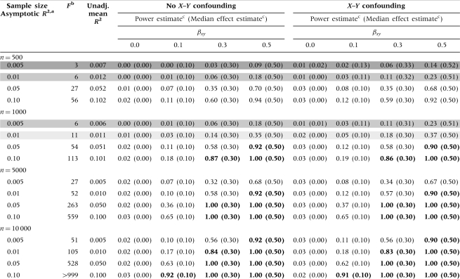^aThis can also be interpreted as the ‘adjusted R²’ for the regression of the exposure (X) on the genetic variant (G).

^bScenarios with weak instrument problems (i.e. low F values) are shown in grey, with darker shading corresponding to lower F values and more bias in the presence of X–Y confounding.

^cPower and median effect estimates were obtained using 10 000 simulations. Scenarios with power >80% are shown in bold. Median effect estimates are shown in parentheses below the power estimates.

Power for MR studies using multiple variants as independent IVs is shown in Table 2. When the adjusted R² is held constant, power and unadjusted R² increase as the number of variants (i.e. IVs) increases, while F decreases. When R² is held constant under no X–Y confounding, there is no impact on power when the number of variants is increased; however, the adjusted R² and F decrease as the number of IVs increases. Each multi-IV scenario has a weak IV problem (shown in grey), resulting in upward bias in the effect estimates in the presence of confounding, especially for very low F values (dark grey). This bias results in power estimates that are artificially inflated compared with the corresponding unconfounded (and unbiased) scenario.

Table 2.

Power, effect estimate and instrument strength (F) comparisons for single- vs multivariant Mendelian randomization studies holding either R² or adjusted R² constant (in bold)

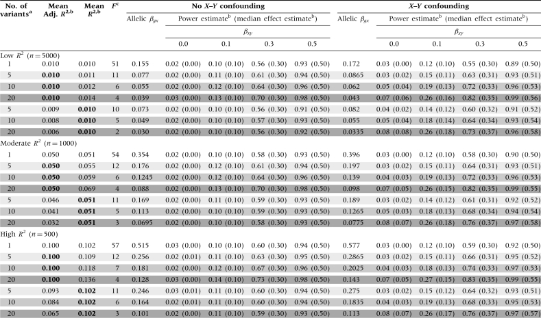^aThe one-variant models have one variant with an X-increaser allele frequency of 0.3. The five-variant models have X-increaser allele frequencies of 0.1, 0.3, 0.5, 0.7 and 0.9. The 10-variant models have two of each of the following X-increaser allele frequencies 0.1, 0.3, 0.5, 0.7 and 0.9. The 20-variant models have four of each of the following X-increaser allele frequencies 0.1, 0.3, 0.5, 0.7 and 0.9.

^bValues were obtained using 10 000 simulations. R² values correspond to the regression of the exposure (X) on the genetic variant(s) (G) and are held constant to the single-variant scenario when shown in bold. Median effect estimates are shown in parentheses below the power estimates.

^cScenarios with weak instrument problems (i.e. low F values) are shown in grey, with darker shading corresponding to lower F values and more bias in the presence of X–Y confounding.

Comparisons of multivariant MR studies using independent IVs vs a composite IV are shown in Table 3. For the unconfounded scenarios, combining variants of equal effect into an X-increaser ‘allele count’ IV resulted in slight decreases in R² and power, when compared with using each G as an independent IV; these decreases becomes more substantial as the number of variants increases. In contrast, combining the variants in to a single IV has no impact on the adjusted R² values, which are identical to the values from the multi-IV scenario. Each multi-IV scenario had a weak IV problem (shaded in grey), again resulting in bias-inflated power estimates under confounding. Using an allele count IV resulted in large increases in F, eliminating the ‘weak-IV’ bias observed in the presence of X–Y confounding.

Table 3.

Power, effect estimate and instrument strength (F) comparisons for Mendelian randomization studies using independent vs combined instruments, holding the per-allele effect size of G on X constant (in bold)

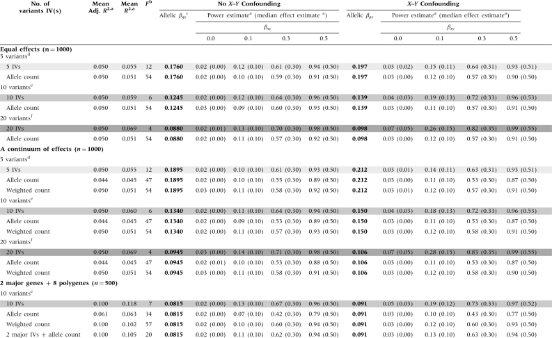^aValues were obtained using 10 000 simulations. R² values correspond to the regression of the exposure (X) on the IV(s). Median effect estimates are shown in parentheses below the power estimates.

^bScenarios with weak instrument problems (i.e. low F values) are shown in grey, with darker shading corresponding to lower F values and more bias in the presence of X–Y confounding.

^cThe allelic β_gx is held constant for all analyses with a specific genetic model (in bold). See the methods section for an interpretation of the allelic β_gx in the ‘continuum of effects’ and the ‘main effects/polygenes’ models.

^dFive variants with the frequencies are 0.1, 0.3, 0.5, 0.7 and 0.9.

^eTen variants total, two with each of the following frequencies: 0.1, 0.3, 0.5, 0.7 and 0.9.

^fTwenty variants total, four with each of the following frequencies: 0.1, 0.3, 0.5, 0.7 and 0.9.

When combining variants with a continuum of effects into a single IV, using an allele count IV increased F, while resulting in decreases for R², adjusted R² and power, compared with the multi-IV scenario (Table 3). Using the ‘weighted allele count’ IV also resulted in large increases in F and decreases in R² and power (compared with the multi-IV scenario), although R² and power estimates greater than those obtained for the allele count IV. The weighted allele count method produced an adjusted R² similar to that obtained from the multi-IV scenario.

When constructing an IV using two variants with ‘major-gene’ effects and eight ‘polygenic’ variants of smaller effect, using an allele count resulted in a substantial decrease in R² and power and a large increase in F (compared with the 10-IV scenario). Using the weighted allele count IV, power was only slightly lower than when using all 10 IVs and the F statistic was much larger. If the variants with large effects were treated as independent IVs and the remaining polygenic variants were combined into a single allele count IV, power was similar to the weighted allele count IV scenario. The F statistic was smaller in this case (mean F = 20), but still >11, resulting in acceptable levels of relative bias (<10%).

Under each model presented in Table 3, introducing positive X–Y confounding results in effect estimates that are biased away from the null and bias-inflated power estimates when compared with the identical model with no X–Y confounding. Table 4 shows the effects of introducing various types of unmeasured X–Y confounding on the estimates from the ‘equal-effects model’. Increasing the strength of the confounding effects increases the magnitude of the bias for the weak IV scenarios. The direction of the bias is always towards the confounded association estimate—away from the null under positive X–Y confounding and towards the null under negative X–Y confounding.

Table 4.

Power^a and effect estimate comparisons for Mendelian randomization studies, varying the strength of X–Y confounding and holding adjusted R² constant (in bold)

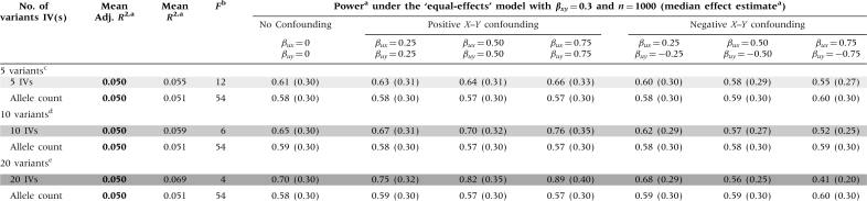^aValues are derived using 10 000 simulations. R² values correspond to the regression of the exposure (X) on the IV(s). Median effect estimates are shown in parentheses below the power estimates.

^bScenarios with weak instrument problems (i.e. low F values) are shown in grey, with darker shading corresponding to lower F values and more bias in the presence of X–Y confounding.

^cFive variants with the frequencies 0.1, 0.3, 0.5, 0.7 and 0.9.

^dTen variants total, two with each of the following frequencies: 0.1, 0.3, 0.5, 0.7 and 0.9.

^eTwenty variants total, four with each of the following frequencies: 0.1, 0.3, 0.5, 0.7 and 0.9.

Discussion

In this simulation study of power and IV strength requirements for MR studies using 2SLS regression, we have evaluated power estimates for single-variant studies over a range of allele frequencies, effect sizes and sample sizes. Our results indicate that well-powered single-IV MR studies are not prone to weak IV problems, and therefore provide unbiased effect estimates in the presence of unmeasured confounding.

For MR studies using multiple variants, we have described the relationships among numerous key study variables, including the number of variants, variant effect sizes, exposure effect sizes, R², adjusted R², F and power. Our results suggest that power to detect a causal effect depends strongly on the R² value of the first-stage regression (not the adjusted R²) and is not influenced by allele frequencies or the number of IVs included in a regression. However, for a fixed R², F decreases as the number of IVs increases, potentially creating weak IV problems (i.e. low F values). The weak IV problem has been extensively described in the econometrics literature.^27–30,33 In short, if an X–Y association is confounded, bias increases as F decreases. This bias is substantial for small F values (~4), but typically becomes negligible for F values >11 (Tables 1–4). This work shows that using each variant as an independent IV results in maximal power, but this strategy is often undesirable because of low F values. The weak IV problem can be overcome by combining the IVs, with modest reductions in power.

We have demonstrated several methods for combining IVs and explored their effects on power. The allele count IV is appropriate when each G has a similar effect, but suboptimal otherwise, as the effect sizes of the variants will be inherently mis-specified. If effect sizes are known, one can calculate a weighted allele count that has only slightly less power than using each variant as an independent IV and avoids weak IV problems. However, this method requires accurate effect estimates derived from previous research on independent samples. An alternative option is to use knowledge regarding ‘major-gene’ and ‘polygenic’ effects to create multiple IVs: one for each variant of large effect, and one representing the collective effects of the variants of small effect. For some circulating proteins, this model could potentially represent cis-effects (which tend to be strong) and trans-effects (which tend to be weak) on gene transcription.³⁴ This model requires no specific information on effect sizes, just knowledge of specific major genes and polygenes.

This work can be better understood in the context of Figure 2, which shows the relationship between R², F, sample size (n) and number of IVs (k) (from Equation 1), in the context of the F thresholds provided by Stock et al.²⁹ A set of IVs with an F below the threshold of ~11 is considered weak and will lead to relative bias >10% in the presence of X–Y confounding, with increasing bias as F decreases. This threshold can be increased or decreased to allow for lower or higher levels of relative bias, respectively.²⁹ Stock and Yogo²⁹ also provide thresholds for F which keep the actual size of the nominal 5% significance test <15% in the presence of ‘maximal’ confounding (i.e. X–Y correlation of 1). Unlike the ‘relative-bias’ threshold used in this work, the ‘actual-size’ threshold increases substantially as the number of IVs increases; however, because such ‘maximal’ confounding is unrealistic for epidemiological applications, we focus on the ‘relative-bias’ threshold in this work.

Figure 2.

Relationship between F and R² for varying sample sizes and number of instrumental variables. The F thresholds from Stock et al.^29,30 are shown as horizontal lines

GWA studies typically identify several weak, independent genetic effects for biomarkers of interest. MR studies utilizing this information will require careful treatment of the weak IV problem, as information on genetic variants of weak effect will often need to be combined to produce strong IVs and an adequately powered MR analysis. The ideal method for translating genetic information into a reasonable number of IVs depends on several factors, including the total number of variants and their relative effect sizes. If using a small number of variants (<5), it may be possible to treat them as independent IVs, depending upon the value of F and the number of IVs.³⁰ This method will maximize power, while making no assumptions regarding the effect sizes of each G. If fewer IVs are needed, the model used to construct the IVs should consider the relative effect size of each G, while attempting to maximize the first-stage R² and F values and minimize the risk of effect-size mis-specification (resulting in loss of power). Models should be based on existing epidemiological and biological evidence.

This work is timely, as GWA studies have recently identified genetic determinants for a wide array of circulating biomarkers with known and suspected roles in a wide array of diseases (e.g. C-reactive protein,^8,9 urate,^35–39 lipids and triglycerides,^5–7 fasting plasma glucose^17–20 and B vitamins^10,11). Clinically relevant physical measures (e.g. blood pressure^15,16 and body mass index^40–42) and life-course traits (e.g. age at menarche and menopause^43–48) have also been shown to have genetic determinants. These variants are often not causal, but in linkage disequilibrium with a causal variant. The proportion of total phenotypic variance in these traits explained by the collective effects of known, common variants (R²) is rarely >0.10 but often >0.01, while some studies fail to report the overall R² for genetic factors. Thus, we have conducted our power analyses using reasonable R² values, in light of current knowledge.

Our simulated data sets were created according to the three key criteria for MR studies: the IV is (i) associated with X, (ii) independent of Y given X and X–Y confounding factors and (iii) independent of factors that confound the X–Y association. Assumption 1 should be well established when conducting an MR study, but Assumptions 2 and 3 may require careful attention. Assumption 2 (known as the ‘exclusion restriction’ in the econometrics literature) requires that G affect Y only through X. This assumption could be violated in the presence of pleiotropy,⁴⁹ where a variant has independent effects on multiple traits (i.e. both X and Y). A violation could also occur if G is in linkage disequilibrium with a nearby variant that affects Y, thereby inducing a correlation between G and Y. It is not possible to test Assumption 2 by testing for G–Y independence while adjusting for X, because this adjustment will induce an association between G and Y in the presence of X–Y confounding (i.e. X is a ‘collider’), even when Assumption 2 is valid; however, this test could be used to assess the absence of X–Y confounding. When using multiple IVs, it is possible to assess Assumption 2 by ensuring the estimates for each IV are similar (the ‘over-identification test’⁵⁰), but this itself requires additional assumptions. Assumption 3 could be violated as a consequence of population stratification, if the distributions of G, X and Y differ between sub-groups of the study sample;⁵¹ however, these differences can be measured and adjusted for using genetic data.³

Our analysis makes several additional simplifying assumptions, namely, additive allelic effects for each variant, no gene–gene interactions and a linear effect for X (on Y). However, if these assumptions were known to be invalid, such knowledge could be incorporated into the model that relates G to the IV(s). For example, for variants with known non-additive effects on X (i.e. dominant or recessive), a binary G variable representing a dominant or recessive effect could be used as an independent IV or as an additional factor included in an allele count. IVs can also be constructed using data on haplotypes^25,26 rather than single variants. Gene–gene interactions could be modelled in a number of ways, including creating independent IVs representing the presence of effects due to interaction or including interaction terms when generating weighted allele counts.

In this analysis, we use the 2SLS regression on simulated cohort data sets to obtain an estimate of the causal effect of X on Y, when both are continuous variables. If there is heterogeneity in the effect of X on Y between individuals then although the 2SLS estimator does give an estimate of the causal effect, its precise interpretation is somewhat complicated.^52,53 The Wald estimator can be used for continuous X and Y variables and produces point estimates identical to the 2SLS method; however, this method cannot accommodate multiple IVs.¹ When the X variable is binary rather than continuous, it is possible to estimate so-called local average treatment or (with additional assumptions) the population average treatment effect.^54,55 When Y is binary, several other methods are available⁵⁶ and a description of some of these for epidemiologists is given in Rassen et al.⁵⁷ These methods include probit structural equation models, two-stage logistic models and generalized method of moments estimators. The biases that can arise with a continuous X and a binary Y are difficult to completely account for using standard statistical methods, although bias can be reduced using a residual-based adjustment in a two-stage logistic model and quantified under varying degrees of hypothesized X–Y confounding using sensitivity analyses.⁵⁸ The causal inference literature has developed methods to handle such settings,^59–61 but these impose an assumption of homogeneity or give only local causal effects. The power calculations derived here are valid only for cohort studies, as case–control studies require analysis techniques that integrate data on disease incidence into the analysis.⁶² For example, if we let π denote the outcome prevalence in the population and we let p denote the ratio of cases to the sum of cases and controls in the study, then to conduct MR analyses with case–control data, we could use standard IV techniques but weight each case by π/p and each control subject by (1−π)/(1−p) to obtain valid results.⁶³

GWA studies are providing new tools for exploring causation using MR studies, but these tools must be applied carefully. The feasibility of MR studies will depend heavily upon the amount of variance in X that can be explained by known genetic factors and our understanding of those genetic effects. Given current knowledge of the genetic determinants of exposures of interest, samples sizes for MR studies will need to be quite large (>1000, sometimes > 10 000). As more is learned regarding the genetics of health-related biomarkers, MR methods may become more efficient and broadly applicable.

Funding

National Institutes of Health (grant numbers UO1 CA122171, RO1 CA107431, RO1 CA102484, P30 CA014599 and P42 ES10349 to H.A.).

Conflict of interest: None declared.

KEY MESSAGES.

• In Mendelian randomization studies, genetic factors that influence an exposure of interest can be used as ‘instrumental variables’ to assess the causality of an exposure–disease association using a two-stage least squares regression.

• Well-powered Mendelian randomization studies will require large (n > 1000), often very large (n > 10 000), sample sizes.

• Using multiple genetic variants as instrumental variables can lead to ‘weak instrument’ scenarios, in which effect estimates may be substantially biased.

• Combining genetic factors into fewer instrumental variable results in modest power decreases, but reduces the ‘weak instrument’ bias.

• Ideal methods for combining genetic factors into fewer instrumental variables depend upon knowledge of the genetic architecture underlying the exposure.

References

- 1.Lawlor DA, Harbord RM, Sterne JA, Timpson N, Davey Smith G. Mendelian randomization: using genes as instruments for making causal inferences in epidemiology. Stat Med. 2008;27:1133–63. doi: 10.1002/sim.3034. [DOI] [PubMed] [Google Scholar]
- 2.Didelez V, Sheehan N. Mendelian randomization as an instrumental variable approach to causal inference. Stat Methods Med Res. 2007;16:309–30. doi: 10.1177/0962280206077743. [DOI] [PubMed] [Google Scholar]
- 3.Tian C, Gregersen PK, Seldin MF. Accounting for ancestry: population substructure and genome-wide association studies. Hum Mol Genet. 2008;17:R143–50. doi: 10.1093/hmg/ddn268. [DOI] [PMC free article] [PubMed] [Google Scholar]
- 4.Wehby GL, Ohsfeldt RL, Murray JC. 'Mendelian randomization' equals instrumental variable analysis with genetic instruments. Stat Med. 2008;27:2745–9. doi: 10.1002/sim.3255. [DOI] [PMC free article] [PubMed] [Google Scholar]
- 5.Aulchenko YS, Ripatti S, Lindqvist I, et al. Loci influencing lipid levels and coronary heart disease risk in 16 European population cohorts. Nat Genet. 2009;41:47–55. doi: 10.1038/ng.269. [DOI] [PMC free article] [PubMed] [Google Scholar]
- 6.Hegele RA. Plasma lipoproteins: genetic influences and clinical implications. Nat Rev Genet. 2009;10:109–21. doi: 10.1038/nrg2481. [DOI] [PubMed] [Google Scholar]
- 7.Kathiresan S, Willer CJ, Peloso GM, et al. Common variants at 30 loci contribute to polygenic dyslipidemia. Nat Genet. 2009;41:56–65. doi: 10.1038/ng.291. [DOI] [PMC free article] [PubMed] [Google Scholar]
- 8.Reiner AP, Barber MJ, Guan Y, et al. Polymorphisms of the HNF1A gene encoding hepatocyte nuclear factor-1 alpha are associated with C-reactive protein. Am J Hum Genet. 2008;82:1193–201. doi: 10.1016/j.ajhg.2008.03.017. [DOI] [PMC free article] [PubMed] [Google Scholar]
- 9.Ridker PM, Pare G, Parker A, et al. Loci related to metabolic-syndrome pathways including LEPR, HNF1A, IL6R, and GCKR associate with plasma C-reactive protein: the Women’s Genome Health Study. Am J Hum Genet. 2008;82:1185–92. doi: 10.1016/j.ajhg.2008.03.015. [DOI] [PMC free article] [PubMed] [Google Scholar]
- 10.Hazra A, Kraft P, Selhub J, et al. Common variants of FUT2 are associated with plasma vitamin B12 levels. Nat Genet. 2008;40:1160–62. doi: 10.1038/ng.210. [DOI] [PMC free article] [PubMed] [Google Scholar]
- 11.Tanaka T, Scheet P, Giusti B, et al. Genome-wide association study of vitamin B6, vitamin B12, folate, and homocysteine blood concentrations. Am J Hum Genet. 2009;84:477–82. doi: 10.1016/j.ajhg.2009.02.011. [DOI] [PMC free article] [PubMed] [Google Scholar]
- 12.Ferrucci L, Perry JR, Matteini A, et al. Common variation in the beta-carotene 15,15'-monooxygenase 1 gene affects circulating levels of carotenoids: a genome-wide association study. Am J Hum Genet. 2009;84:123–33. doi: 10.1016/j.ajhg.2008.12.019. [DOI] [PMC free article] [PubMed] [Google Scholar]
- 13.Meisinger C, Prokisch H, Gieger C, et al. A genome-wide association study identifies three loci associated with mean platelet volume. Am J Hum Genet. 2009;84:66–71. doi: 10.1016/j.ajhg.2008.11.015. [DOI] [PMC free article] [PubMed] [Google Scholar]
- 14.Soranzo N, Rendon A, Gieger C, et al. A novel variant on chromosome 7q22.3 associated with mean platelet volume, counts, and function. Blood. 2009;113:3831–37. doi: 10.1182/blood-2008-10-184234. [DOI] [PMC free article] [PubMed] [Google Scholar]
- 15.Levy D, Ehret GB, Rice K, et al. Genome-wide association study of blood pressure and hypertension. Nat Genet. 2009;41:677–87. doi: 10.1038/ng.384. [DOI] [PMC free article] [PubMed] [Google Scholar]
- 16.Newton-Cheh C, Johnson T, Gateva V, et al. Genome-wide association study identifies eight loci associated with blood pressure. Nat Genet. 2009;41:666–76. doi: 10.1038/ng.361. [DOI] [PMC free article] [PubMed] [Google Scholar]
- 17.Bouatia-Naji N, Bonnefond A, Cavalcanti-Proenca C, et al. A variant near MTNR1B is associated with increased fasting plasma glucose levels and type 2 diabetes risk. Nat Genet. 2009;41:89–94. doi: 10.1038/ng.277. [DOI] [PubMed] [Google Scholar]
- 18.Bouatia-Naji N, Rocheleau G, Van Lommel L, et al. A polymorphism within the G6PC2 gene is associated with fasting plasma glucose levels. Science. 2008;320:1085–88. doi: 10.1126/science.1156849. [DOI] [PubMed] [Google Scholar]
- 19.Chen WM, Erdos MR, Jackson AU, et al. Variations in the G6PC2/ABCB11 genomic region are associated with fasting glucose levels. J Clin Invest. 2008;118:2620–28. doi: 10.1172/JCI34566. [DOI] [PMC free article] [PubMed] [Google Scholar]
- 20.Prokopenko I, Langenberg C, Florez JC, et al. Variants in MTNR1B influence fasting glucose levels. Nat Genet. 2009;41:77–81. doi: 10.1038/ng.290. [DOI] [PMC free article] [PubMed] [Google Scholar]
- 21.Cho YS, Go MJ, Kim YJ, et al. A large-scale genome-wide association study of Asian populations uncovers genetic factors influencing eight quantitative traits. Nat Genet. 2009;41:527–34. doi: 10.1038/ng.357. [DOI] [PubMed] [Google Scholar]
- 22.Melzer D, Perry JR, Hernandez D, et al. A genome-wide association study identifies protein quantitative trait loci (pQTLs) PLoS Genet. 2008;4:e1000072. doi: 10.1371/journal.pgen.1000072. [DOI] [PMC free article] [PubMed] [Google Scholar]
- 23.Sabatti C, Service SK, Hartikainen AL, et al. Genome-wide association analysis of metabolic traits in a birth cohort from a founder population. Nat Genet. 2009;41:35–46. doi: 10.1038/ng.271. [DOI] [PMC free article] [PubMed] [Google Scholar]
- 24.Yuan X, Waterworth D, Perry JR, et al. Population-based genome-wide association studies reveal six loci influencing plasma levels of liver enzymes. Am J Hum Genet. 2008;83:520–28. doi: 10.1016/j.ajhg.2008.09.012. [DOI] [PMC free article] [PubMed] [Google Scholar]
- 25.Brunner EJ, Kivimaki M, Witte DR, et al. Inflammation, insulin resistance, and diabetes–Mendelian randomization using CRP haplotypes points upstream. PLoS Med. 2008;5:e155. doi: 10.1371/journal.pmed.0050155. [DOI] [PMC free article] [PubMed] [Google Scholar]
- 26.Timpson NJ, Lawlor DA, Harbord RM, et al. C-reactive protein and its role in metabolic syndrome: Mendelian randomisation study. Lancet. 2005;366:1954–59. doi: 10.1016/S0140-6736(05)67786-0. [DOI] [PubMed] [Google Scholar]
- 27.Bound J, Jaeger DA, Baker RM. Problems with instrumental variables estimation when the correlation between the instruments and the endogeneous explanatory variable is weak. J Am Statist Assoc. 1995;90:443–50. [Google Scholar]
- 28.Nelson CR, Startz R. The distribution of the instrumental variables estimator and its t-ratio when the instrument is a poor one. J Bus. 1990;63:S125–40. [Google Scholar]
- 29.Stock JH, Yogo M. Testing for Weak Instruments in Linear IV Regression. Cambridge, MA: National Bureau of Economic Research, Inc; 2002. [Google Scholar]
- 30.Stock JH, Wright JH, Yogo M. A survey of weak instruments and weak identification in generalized method of moments. J Bus Econ Statist. 2002;20:518–29. [Google Scholar]
- 31.Staiger D, Stock JH. Instrumental Variables Regression with Weak Instruments. Cambridge, MA: National Bureau of Economic Research, Inc.; 1994. [Google Scholar]
- 32.Draper NR, Smith H. Applied Regression Analysis. New York: Wiley-Interscience; 1998. [Google Scholar]
- 33.Donald SG, Newey WK. Choosing the number of instruments. Econometrica. 2001;69:1161–91. [Google Scholar]
- 34.Gilad Y, Rifkin SA, Pritchard JK. Revealing the architecture of gene regulation: the promise of eQTL studies. Trends Genet. 2008;24:408–15. doi: 10.1016/j.tig.2008.06.001. [DOI] [PMC free article] [PubMed] [Google Scholar]
- 35.Dehghan A, Kottgen A, Yang Q, et al. Association of three genetic loci with uric acid concentration and risk of gout: a genome-wide association study. Lancet. 2008;372:1953–61. doi: 10.1016/S0140-6736(08)61343-4. [DOI] [PMC free article] [PubMed] [Google Scholar]
- 36.Doring A, Gieger C, Mehta D, et al. SLC2A9 influences uric acid concentrations with pronounced sex-specific effects. Nat Genet. 2008;40:430–36. doi: 10.1038/ng.107. [DOI] [PubMed] [Google Scholar]
- 37.Vitart V, Rudan I, Hayward C, et al. SLC2A9 is a newly identified urate transporter influencing serum urate concentration, urate excretion and gout. Nat Genet. 2008;40:437–42. doi: 10.1038/ng.106. [DOI] [PubMed] [Google Scholar]
- 38.Wallace C, Newhouse SJ, Braund P, et al. Genome-wide association study identifies genes for biomarkers of cardiovascular disease: serum urate and dyslipidemia. Am J Hum Genet. 2008;82:139–49. doi: 10.1016/j.ajhg.2007.11.001. [DOI] [PMC free article] [PubMed] [Google Scholar]
- 39.Li S, Sanna S, Maschio A, et al. The GLUT9 gene is associated with serum uric acid levels in Sardinia and Chianti cohorts. PLoS Genet. 2007;3:e194. doi: 10.1371/journal.pgen.0030194. [DOI] [PMC free article] [PubMed] [Google Scholar]
- 40.Meyre D, Delplanque J, Chevre JC, et al. Genome-wide association study for early-onset and morbid adult obesity identifies three new risk loci in European populations. Nat Genet. 2009;41:157–59. doi: 10.1038/ng.301. [DOI] [PubMed] [Google Scholar]
- 41.Thorleifsson G, Walters GB, Gudbjartsson DF, et al. Genome-wide association yields new sequence variants at seven loci that associate with measures of obesity. Nat Genet. 2009;41:18–24. doi: 10.1038/ng.274. [DOI] [PubMed] [Google Scholar]
- 42.Willer CJ, Speliotes EK, Loos RJ, et al. Six new loci associated with body mass index highlight a neuronal influence on body weight regulation. Nat Genet. 2009;41:25–34. doi: 10.1038/ng.287. [DOI] [PMC free article] [PubMed] [Google Scholar]
- 43.He C, Kraft P, Chen C, et al. Genome-wide association studies identify loci associated with age at menarche and age at natural menopause. Nat Genet. 2009;41:724–8. doi: 10.1038/ng.385. [DOI] [PMC free article] [PubMed] [Google Scholar]
- 44.Liu YZ, Guo YF, Wang L, et al. Genome-wide association analyses identify SPOCK as a key novel gene underlying age at menarche. PLoS Genet. 2009;5:e1000420. doi: 10.1371/journal.pgen.1000420. [DOI] [PMC free article] [PubMed] [Google Scholar]
- 45.Ong KK, Elks CE, Li S, et al. Genetic variation in LIN28B is associated with the timing of puberty. Nat Genet. 2009;41:729–33. doi: 10.1038/ng.382. [DOI] [PMC free article] [PubMed] [Google Scholar]
- 46.Perry JR, Stolk L, Franceschini N, et al. Meta-analysis of genome-wide association data identifies two loci influencing age at menarche. Nat Genet. 2009;41:648–50. doi: 10.1038/ng.386. [DOI] [PMC free article] [PubMed] [Google Scholar]
- 47.Sulem P, Gudbjartsson DF, Rafnar T, et al. Genome-wide association study identifies sequence variants on 6q21 associated with age at menarche. Nat Genet. 2009;41:634–8. doi: 10.1038/ng.383. [DOI] [PubMed] [Google Scholar]
- 48.Stolk L, Zhai G, van Meurs JB, et al. Loci at chromosomes 13, 19 and 20 influence age at natural menopause. Nat Genet. 2009;41:645–7. doi: 10.1038/ng.387. [DOI] [PMC free article] [PubMed] [Google Scholar]
- 49.Thomas DC, Conti DV. Commentary: the concept of ‘Mendelian Randomization’. Int J Epidemiol. 2004;33:21–25. doi: 10.1093/ije/dyh048. [DOI] [PubMed] [Google Scholar]
- 50.Baum CF, Schaffer ME, Stillman S. Instrumental variables and GMM: estimation and testing. Stata J. 2003;3:1–31. [Google Scholar]
- 51.Little J, Khoury MJ. Mendelian randomisation: a new spin or real progress? Lancet. 2003;362:930–31. doi: 10.1016/S0140-6736(03)14396-6. [DOI] [PubMed] [Google Scholar]
- 52.Angrist JD, Imbens GW. Two-stage least squares estimation of average causal effects in models with variable treatment intensity. J Am Statist Assoc. 1995;90:431–42. [Google Scholar]
- 53.Heckman JJ, Vytlacil EJ. Structural equations, treatment effects, and econometric policy evaluation. Econometrica. 2005;73:669–738. [Google Scholar]
- 54.Imbens GW, Angrist JD. Identification and estimation of local average treatment effects. Econometrica. 1994;62:467–75. [Google Scholar]
- 55.Tan Z. Regression and weighting methods for causal inference using instrumental variables. J Am Statist Assoc. 2006;101:1607–18. [Google Scholar]
- 56.Greene WH. Econometric Analysis. 5th. Upper Saddle River, NJ: Prentice Hall; 2003. [Google Scholar]
- 57.Rassen JA, Schneeweiss S, Glynn RJ, Mittleman MA, Brookhart MA. Instrumental variable analysis for estimation of treatment effects with dichotomous outcomes. Am J Epidemiol. 2009;169:273–84. doi: 10.1093/aje/kwn299. [DOI] [PubMed] [Google Scholar]
- 58.Palmer TM, Thompson JR, Tobin MD, Sheehan NA, Burton PR. Adjusting for bias and unmeasured confounding in Mendelian randomization studies with binary responses. Int J Epidemiol. 2008;37:1161–68. doi: 10.1093/ije/dyn080. [DOI] [PubMed] [Google Scholar]
- 59.Robins JM, Rotnitzky A. Estimation of treatment effects in randomised trials with non-compliance and a dichotomous outcome using structural mean models. Biometrika. 2004;91:763–83. [Google Scholar]
- 60.van der Laan MJ, Hubbard A, Jewell NP. Estimation of treatment effects in randomized trials with noncompliance and a dichotomous outcome. J R Stat Soc B. 2007;69:442–82. [Google Scholar]
- 61.Vansteelandt S, Goetghebeur E. Causal inference with generalized structural mean models. J R Stat Soc B. 2003;65:817–35. [Google Scholar]
- 62.Shinohara RT, Frangakis CE, Platz E, Tsilidis K. Estimating Effects by Combining Instrumental Variables with Case-control Designs: the Role of Principal Stratification. Johns Hopkins University, Dept of Biostatistics Working Papers; 2008. (Working Paper 198): http://www.bepress.com/jhubiostat/paper198 (1 November 2009, date last accessed) [Google Scholar]
- 63.Van der Laan MJ. Estimation based on case-control designs with known prevalence probability. Int J Biostat. 2008;4:Article 17. doi: 10.2202/1557-4679.1114. [DOI] [PubMed] [Google Scholar]