Multinomial Logistic Functions in Markov Chain Models of Sleep Architecture: Internal and External Validation and Covariate Analysis

Abstract

Mixed-effect Markov chain models have been recently proposed to characterize the time course of transition probabilities between sleep stages in insomniac patients. The most recent one, based on multinomial logistic functions, was used as a base to develop a final model combining the strengths of the existing ones. This final model was validated on placebo data applying also new diagnostic methods and then used for the inclusion of potential age, gender, and BMI effects. Internal validation was performed through simplified posterior predictive check (sPPC), visual predictive check (VPC) for categorical data, and new visual methods based on stochastic simulation and estimation and called visual estimation check (VEC). External validation mainly relied on the evaluation of the objective function value and sPPC. Covariate effects were identified through stepwise covariate modeling within NONMEM VI. New model features were introduced in the model, providing significant sPPC improvements. Outcomes from VPC, VEC, and external validation were generally very good. Age, gender, and BMI were found to be statistically significant covariates, but their inclusion did not improve substantially the model’s predictive performance. In summary, an improved model for sleep internal architecture has been developed and suitably validated in insomniac patients treated with placebo. Thereafter, covariate effects have been included into the final model.

Electronic supplementary material

The online version of this article (doi:10.1208/s12248-011-9287-4) contains supplementary material, which is available to authorized users.

INTRODUCTION

Sleep disorders affect a large portion of the world’s population—prevalence is thought to be approximately 10% (1)—and their effects are far-reaching: medical, psychiatric, personal, and societal spheres are all substantially involved. Among other things, sleep pathologies affect the quality of life because of comorbid conditions and impaired interpersonal relationships (1).

The appropriate diagnosis and treatment of these disorders still represent great challenges for clinicians and pharmaceutical companies. The latter have made large investments in this research field, trying to develop safer and more effective drugs able to regulate the sleep–wake alternation. But it is of particular importance that the therapeutic interventions also maintain the physiological sleep architecture (2,3), which is a physiologically relevant description of the sequence of sleep stages (REM, slow-wave sleep, awake, etc.) coming one after the other during nighttime. An individual sleep pattern can be easily assessed through polysomnography (4), but its characterization in a population is problematic: the data to describe are categorical, non-ordered, and with high variability between subjects and occasions.

Different models have been proposed to characterize the time course of sleep stages in groups of individuals, in particular those by Karlsson et al. (5), Kjellsson et al. (6), and Bizzotto et al. (7): all of them used Markov chains for describing the time course of transition probabilities between sleep stages in insomnia patients. Karlsson et al. introduced Markov chain models as tools for describing sleep data, included the so-called stage time effects, and parameterized the models through binary logistic functions. Bizzotto et al. introduced multinomial logistic functions instead of the binary ones, without including stage time effect. Kjellsson et al. described initial sleeplessness as a new sleep stage and estimated the knots of the piecewise linear binary logits instead of fixing them. These are, briefly, the strengths of the existing models for the time course of sleep stages, which will be clarified in “MATERIALS AND METHODS.”

The objectives of the present work were therefore to (1) build on and combine these features, (2) add additional components, and (3) perform a fuller model validation than before using partly new diagnostic methods. In the general scope of improving the proposed models, we also aimed to reduce the model structure without compromising the model performance in describing the data in order to include potential covariate and drug effects.

We internally validated the final model against the original dataset using two traditional visual diagnostics for categorical data: the visual predictive check (VPC) (8) and a check closely related to posterior predictive check, already implemented in (5) and called here simplified posterior predictive check (sPPC). In addition, a new diagnostic was introduced in this work to assess the accuracy and precision of model parameter estimates through a graphic description of transition probability time courses: the visual estimation check (VEC). The final Markov chain model was also externally validated on a new study not used for the model development.

Finally, we used the proposed model to explore covariate effects (age, gender, and BMI) on transition probabilities between sleep stages. In the literature, such analysis was reported only for some specific aggregated sleep parameters, e.g., total sleep time, number of arousals, etc. (9–15). A sounder inspection on the entire sleep architecture was instead not possible since appropriate models were not available.

MATERIALS AND METHODS

Clinical Studies

Data were obtained from the placebo arms of two polysomnographic (PSG) multicentre, randomized, double-blind, placebo-controlled parallel group studies designed to investigate two new candidate drugs. These two studies (A and B) followed a similar design, reported in Bizzotto et al. (7) for study A. The only difference was in the inclusion criteria for the PSG parameters, described as follows. The mean sleep parameter values obtained in the two screening PSGs (with single-blinded placebo administration) had to fall within the following ranges: mean total sleep time (TST) between 240 and 390 min in study A and between 240 and 420 min in study B; mean latency to persistent sleep (LPS) of at least 30 min and not less than 20 min on either night (study A), and mean LPS of at least 20 min and not less than 15 min on either night (study B). Mean wake after sleep onset (WASO) was instead the same in both studies, i.e., 60 min or more and neither night <45 min.

Age, gender, and body mass index (BMI) were available for each patient from studies A and B. Demographic statistics are reported in Electronic Supplementary Material (ESM) Table I.

Datasets

Data from study A were used to develop the Markov chain model, internally validate the model, and perform covariate analysis. Data from study B were used for external validation only. The two datasets included PSG measurements from the first night of treatment in the placebo arm: N_A = 116 subjects in study A and N_B = 81 subjects in study B. Each measure reported the sleep stage of a specific subject in a 30-s time interval, called “epoch.” PSG signals were recorded for 8 h along the night. The considered sleep stages were the awake one (AW), stages 1 and 2 of light sleep (ST1 and ST2), deep sleep or slow-wave sleep (SWS), and rapid eye movement sleep (REM), as reported by Rechtschaffen and Kales (4).

Base Multinomial Markov Chain Model

In this section, we present the so-called base multinomial Markov chain model whose structure, derived from Bizzotto et al. (7), was the framework into which the strengths of models presented by Karlsson et al. (5) and Kjellsson et al. (6) were incorporated. In the following, we denote s_it as the state (i.e., sleep stage) of a subject i at epoch t (also called “nighttime”), taking finite values in the set S = {AW, ST1, ST2, SWS, REM} of sleep stages. Moreover, we denote as the probability of the transition between state k at nighttime t − 1 and state m at nighttime t. The parameterization of the model relies on the introduction of multinomial logit functions, , defined as the following for all i ∈ {1,…, N}, k, m, and r ∈ S, and t ∈ {1,…, n}:

1

In the above definition, the choice of r, called “reference state,” is a degree of freedom that may be exploited to improve model performance.

The vectors , k ∈ S, i ∈ {1,…, N}, t ∈ {1,…, n} completely describe the model. For each k in S, such vectors are characterized in an independent sub-model, referred to as “sub-model k”. Logit function values for the different individuals are assumed normally distributed, i.e.,

2

where is the vector of typical values of the logit functions and is a diagonal covariance matrix for inter-individual variability. The relationship between logits and nighttime is modeled through piecewise linear functions, making the Markov chains non-homogeneous.

Model Development

The aim of the model development strategy was to improve the multinomial Markov chain model previously proposed (7) in order to facilitate the assessment of covariate and drug effects and reduce potential model biases. Each step in model development was tested through sPPC (described below) and through parsimony criteria, i.e., log-likelihood ratio test, with hierarchical structures, and Bayesian information criterion (BIC), with non-hierarchical structures. Consistency between sub-models was always preferred when these criteria were suggesting slightly different developments in the different sub-models.

Model reduction was attempted by decreasing the number of knots (called “break points”) in the piecewise logit functions and zeroing some transition probabilities. The removal of model biases was instead pursued acting on different model features, first of all the value of the reference state r to be used for each triple (i, k, t) in Eq. 1. Then, the significance of values different from zero was tested for each variance–covariance element in the full . Since internal validation showed some misspecifications related to SWS (see “RESULTS”), and SWS epochs often follow or precede ST2 epochs, a new sub-model was introduced by merging sub-models ST2 and SWS: in this new sub-model correlation, terms were tested between individual values of logits defined on ST2 and SWS leaving stages. Finally, in order to convey a more physiological characterization of sleep architecture, two model features implemented by Karlsson et al. (5) and Kjellsson et al. (6) in their Markov chain models with binary logit functions were introduced in this model (with multinomial logit functions) and tested on our data. The main purpose of such features was to relax the first-order assumption made on the Markov chain model. The first feature is letting the logits depend also on other variables, in addition to nighttime: both time elapsed since the last change in sleep stage (“stage time”) and time elapsed in a sleep stage since the nighttime beginning (the latter never tested in the literature) were attempted. The second feature is the differentiation of the model behavior between initial sleeplessness and rest of nighttime.

The identification of the sub-models was performed using NONMEM VI (Globomax Corp.) (16).

Internal Validation

Internal validation was implemented according to multiple techniques (using data from study A). Each of them was based on Monte Carlo simulation of 100 datasets from the identified and merged sub-models, with number of individuals as in the original study.

Simplified Posterior Predictive Check

sPPC was performed to assess the model’s capability in describing and simulating aggregated characteristics of PSG data in the population. This technique was used during the whole model development process. Several aggregated parameters of clinical interest in detecting hypnotics efficacy were considered (e.g., WASO, TST, LPS) (7). The individual values of each of these parameters, derived from the observed data, were compared with the corresponding values computed from the simulated data. In particular, for any given parameter, the median of the individual values was computed in each dataset (observed or simulated); the relative deviations of medians were calculated as follows:

3

For each endpoint, the distribution of relative deviations was computed and plotted in box–whisker plots using the R package (R 2.10.0 from the R Development Core, 2009).

Visual Predictive Check

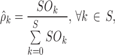
The final model capability in describing the physiological evolution of the sleep stages and transitions along nighttime was tested through VPC (17). Two new statistics computed on the observed data together with the corresponding confidence interval derived from simulations (the ones used for sPPC) were plotted against nighttime t. These statistics were the frequencies of occurrence of each sleep stage (as proposed in Bergstrand et al. (8) for categorical data):

4

where is the number of occurrences of state k in the dataset; and the transition frequencies between stages:

5

where N_km is the number of transitions from state k to state m in the dataset and N_k is the number of transitions from state k. Each statistic was computed for each of ten equal intervals in the nighttime (48 min each).

Visual Estimation Check

The VEC is a novel approach to assess the robustness and precision of parameter estimates in terms of transition probability time course, and it is introduced in this work. It relies on the combination of stochastic simulation, re-estimation (18,19), and computation. Specifically, all of the 100 simulated datasets were re-identified using the developed Markov sub-models. From each of the original and the simulated datasets, the estimated parameter values were used for computing the temporal profiles of typical transition probabilities, and for drawing and computing the temporal profiles of individual transition probabilities, from which 5th and 95th percentiles were derived. Consequently, an observed and 100 simulated profiles were obtained to evaluate three statistics: the typical transition probabilities and the 5th and 95th percentiles on inter-individual variability. At the end, the 95% confidence intervals for each statistic profile derived from the simulation were computed and visually compared with each observed statistic profile.

External Validation

The external validation of the final model was performed applying the model to data from study B and looking at objective function values (OFVs), distributions of empirical Bayes estimates (EBEs), parameter values, and sPPC. OFV and EBE distributions were computed for dataset B using each of the five sub-models in two different scenarios: using parameter values estimated from study A and using parameter values estimated from study B. sPPC was performed comparing aggregated parameters computed on study B with the corresponding aggregated parameters computed on 100 datasets simulated from parameter values estimated on study B.

Covariate Selection

The last objectives of this work were (1) the identification of the appropriate structural form of a second-stage model for defining the covariate effects and (2) the evaluation of the statistical relevance of the covariate, tested on study A using stepwise covariate modeling (20). The chosen discriminating p values for covariate effect inclusion (forward search) and exclusion (backward search) were 0.05 and 0.01, respectively. Linear and piecewise linear additive effects were tested on each logit at each different nighttime break point. Different effects at different break points were allowed.

RESULTS

Model Development

Reference Stage

The exploration of the value of the reference state r to be used in brought to the choice of the same value used for k. Accordingly, r disappears from the logit notation; Eq. 1 can be rewritten as:

6

and Eq. 2 becomes

7

Actually, this choice was supported by parsimony considerations (lower objective function values) within sub-models AW, ST2, SWS, and REM. The reference state for sub-model ST1 providing the lowest objective function value was ST2, but little difference derived from using ST1 instead; thus, the latter state was chosen in order to achieve complete consistency among sub-models.

Transition Probabilities Fixed to Zero

Transitions for which probability could be fixed to zero were chosen according to their observed frequency (Eq. 5). The chosen frequency threshold was 0.1%. Consequently, the number of logits in each sub-model was reduced as reported in Table I.

Table I.

Logits for the Different Sub-models

AW	ST1	ST2	SWS	REM
0	1: g iST1AW(t)	1: g iST2AW(t)	1: g iSWSAW(t)	1: g iREMAW(t)
1: g iAWST1(t)	0	2: g iST2ST1(t)	2: g iSWSST1(t)	2: g iREMST1(t)
2: g iAWST2(t)	2: g iST1ST2(t)	0	3: g iSWSST2(t)	3: g iREMST2(t)
–	–	3: g iST2SWS(t)	0	–
3: g iAWREM(t)	3: g iST1REM(t)	4: g iST2REM(t)	–	0

Nighttime Break Points

The number of break points in the piecewise linear logit functions of nighttime was reduced from 6 to 3, BPA, BPB, and BPC: BPA and BPC were placed at the nighttime beginning (epoch 2) and end (epoch 960), respectively, and BPB was estimated in each sub-model as a new parameter (with no inter-individual variability), as suggested in (6) for binary logit functions. Consequently, the individual logits at the break points can be expressed with the vector:

8

where are the typical individual values of the logit km at times BPA, BPB, and BPC, and is the individual deviation from this logit.

Once nighttime break points are introduced, the matrices , in Eq. 7, are replaced by , with elements

9

Inter-individual Variability

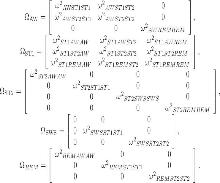
The search for triples (k, m, n) bringing to values of statistically different from zero in the full brought to the use of the following variance–covariance matrices:

10

No significant improvements were achieved by introducing correlation terms between individual logits in sub-model ST2-SWS (unification of sub-models ST2 and SWS); therefore, these parameters were not included in the final model.

Stage Time Effect

Stage time t_s was assumed to modify each logit at its three nighttime break points according to an additive piecewise linear model. Three break points for each sub-model k were again chosen for the stage time effect, : BPsa at t_s = 1 epoch (the minimum stage time that can be observed), BPsc at the maximum observed time elapsed since the last change in state k, and BPsb considered as a model parameter constrained in the interval (BPsa, BPsc). Therefore, the vector of individual logits at the nighttime break points (Eq. 8) becomes a function of t_s:

11

The introduction of time elapsed in a sleep stage since nighttime beginning did not produce significant improvements; therefore, this predictor was not included in the final model.

Initial Sleeplessness

In sub-model AW, the 8-h nighttime was divided into two parts: the first part ranged from the beginning of nighttime to t = IS, where IS is the first epoch of the night in which a non-awake state is observed in a specific subject, and the second one covered the remaining part of the night. In the second time interval, the logits were modeled as previously described, changing only the position of the first nighttime break point: BPA = IS. During initial sleeplessness, new logits were modeled, again as piecewise linear functions, but without inter-individual variability or stage time effects. In particular, three additional break points were defined: BP1 at nighttime beginning (epoch 2), BP3 at the maximum IS observed in the data for the specific sub-model, and the central BP2 considered as a model parameter. When referring to initial sleeplessness, the vector in Eq. 11, which defines the individual logits at the nighttime break points, is thus expressed as follows:

12

where are the values of the logit km at times BP1, BP2, and BP3. The feasibility of using IS as the first epoch of persistent sleep was also tested, but not supported by the data.

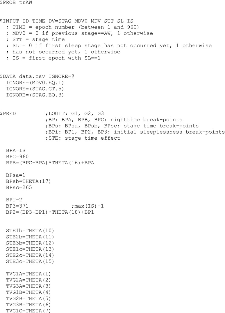
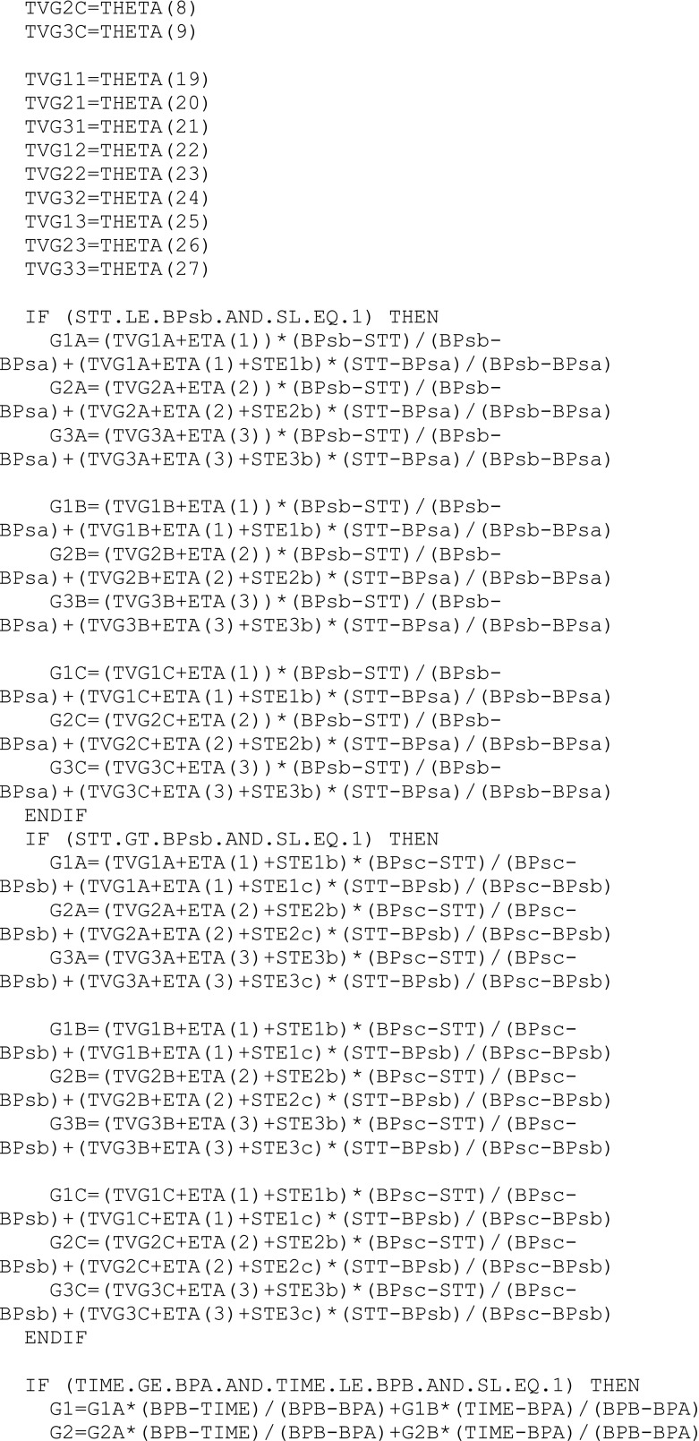
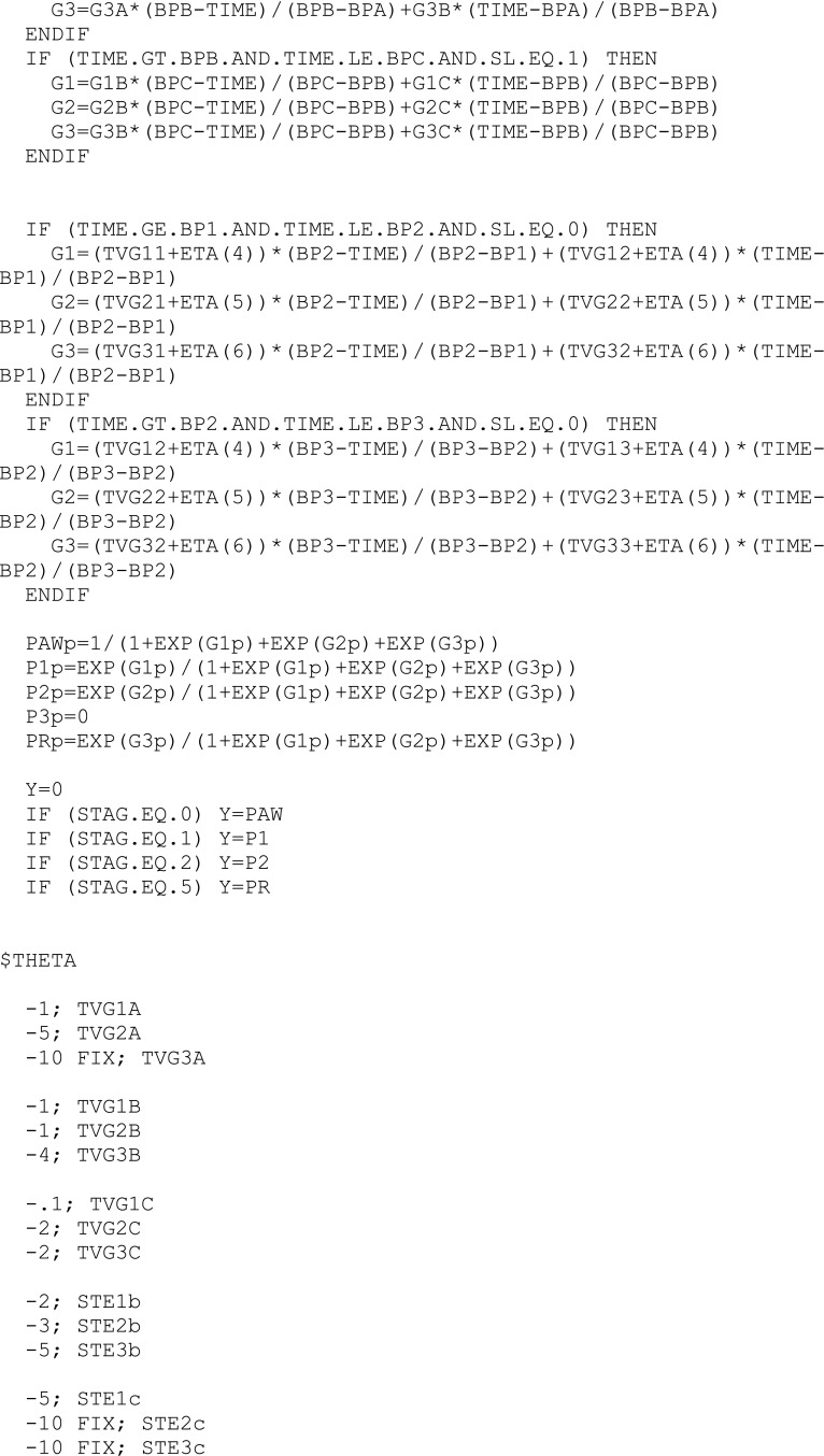
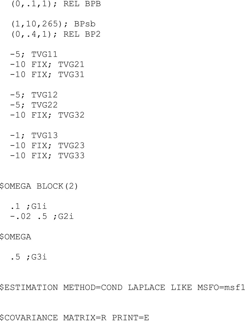
A final model file, the one for estimating sub-model AW, is shown in Appendix 1 as an example, and some lines of the data file used for that control stream are shown in Appendix 2. Condition numbers for the final sub-models were in the range 6.9–25.8 (they were not available for the base sub-models (7) since the R matrix, i.e., the inverse Hessian, could not be computed in those cases).

The estimated parameter values are shown in Table II. Eight parameters, involved in the computation of logits defined on ratios close to zero in sub-model AW, had to be fixed to −10, a value which is close enough to zero in terms of probability ratios. When these parameters were not considered fixed, they had high CVs and likelihood minimization by NONMEM was rarely successful. However, they could not be discarded because they were involved in limited time intervals (nighttime or stage time) and the piecewise linear functions of time needed to be defined in their entire domain.

Table II.

Model Parameter Values Estimated from Study A

Sub-model	Parameters	Parameter labels and values
AW	Logits at nighttime break points	g AWST1A	g AWST2A	g AWREMA	g AWST1B	g AWST2B	g AWREMB	g AWST1C	g AWST2C	g AWREMC
		−0.251	−2.66	−10 FIX	−0.209	−1.01	−2.86	−0.203	−2.08	−2.1
	Logits at initial sleeplessness break points	g AWST11	g AWST21	g AWREM1	g AWST12	g AWST22	g AWREM2	g AWST13	g AWST23	g AWREM3
		−5.76	−10 FIX	−10 FIX	−3.93	−7.63	−10 FIX	−4.86	−10 FIX	−10 FIX
	Stage time effects at stage time break points	s AWST1(BPsb)	s AWST2(BPsb)	s AWREM(BPsb)	s AWST1(BPsc)	s AWST2(BPsc)	s AWREM(BPsc)
		−2.49	−3.59	−5.67	−6.63	−10 FIX	−10 FIX
	Break points	BPAa	BPB	BPCa	BPsaa	BPsb	BPsca	BP1a	BP2	BP3a
		ISb	0.0679c	960 FIX	1 FIX	7.32	265 FIX	2 FIX	13.00	371 FIX
	Var–covar for inter-individual variability	ω 2 AWST1ST1	ω 2 AWST2ST1	ω 2 AWST2ST2	ω 2 AWREMREM
		0.134	−0.142	0.831	1.07
ST1	Logits at nighttime break points	g ST1AWA	g ST1ST2A	g ST1REMA	g ST1AWB	g ST1ST2B	g ST1REMB	g ST1AWC	g ST1ST2C	g ST1REMC
		−0.321	−0.0716	−4.15	−1.07	0.492	−1.01	−1.05	−0.251	−1.24
	Stage time effects at stage time break points	s ST1AW(BPsb)	s ST1ST2(BPsb)	s ST1REM(BPsb)	s ST1AW(BPsc)	s ST1ST2(BPsc)	s ST1REM(BPsc)
		−0.447	−0.52	−0.463	−0.634	−0.246	−3.31
	Break points	BPAa	BPB	BPCa	BPsaa	BPsb	BPsca
		2 FIX	268	960 FIX	1 FIX	3.24	20 FIX
	Var–covar for inter-individual variability	ω 2 ST1AWAW	ω 2 ST1ST2AW	ω 2 ST1ST2ST2	ω 2 ST1REMAW	ω 2 ST1REMST2	ω 2 ST1REMREM
		0.318	0.18	0.389	−0.0637	0.138	0.398
ST2	Logits at nighttime break points (1)	g ST2AWA	g ST2ST1A	g ST2SWSA	g ST2REMA	g ST2AWB	g ST2ST1B	g ST2SWSB	g ST2REMB
		−2.46	−2.52	−1.71	−4.07	−2.57	−2.6	−3.33	−3.34
	Logits at nighttime break points (2)	g ST2AWC	g ST2ST1C	g ST2SWSC	g ST2REMC
		−2.13	−2.33	−4.59	−3.16
	Stage time effects at stage time break points	s ST2AW(BPsb)	s ST2ST1(BPsb)	s ST2SWS(BPsb)	s ST2REM(BPsb)	s ST2AW(BPsc)	s ST2ST1(BPsc)	s ST2SWS(BPsc)	s ST2REM(BPsc)
		−0.905	−0.894	−1.19	−0.993	−1.79	−6.44	0.927	−6.75
	Break points	BPAa	BPB	BPCa	BPsaa	BPsb	BPsca
		2 FIX	676	960 FIX	1 FIX	5.62	143 FIX
	Var–covar for inter-individual variability	ω 2 ST2AWAW	ω 2 ST2ST1ST1	ω 2 ST2SWSSWS	ω 2 ST2REMREM
		0.152	0.456	0.786	0.239
SWS	Logits at nighttime break points	g SWSAWA	g SWSST1A	g SWSST2A	g SWSAWB	g SWSST1B	g SWSST2B	g SWSAWC	g SWSST1C	g SWSST2C
		−3.22	−4.83	−0.526	−3.31	−5.13	0.142	−1.65	−4.55	0.389
	Stage time effects at stage time break points	s SWSAW(BPsb)	s SWSST1(BPsb)	s SWSST2(BPsb)	s SWSAW(BPsc)	s SWSST1(BPsc)	s SWSST2(BPsc)
		−0.999	−0.939	−2.5	0.761	−3.53	−3.73
	Break points	BPAa	BPB	BPCa	BPsaa	BPsb	BPsca
		2 FIX	715	960 FIX	1 FIX	5.9	103 FIX
	Var–covar for inter-individual variability	ω 2 SWSST1ST1	ω 2 SWSST2ST2
		1.4	1.35
REM	Logits at nighttime break points	g REMAWA	g REMST1A	g REMST2A	g REMAWB	g REMST1B	g REMST2B	g REMAWC	g REMST1C	g REMST2C
		−3.12	−2.87	−3.11	−3.25	−3.02	−4.6	−2.96	−2.98	−4.56
	Stage time effects at stage time break points	s REMAW(BPsb)	s REMST1(BPsb)	s REMST2(BPsb)	s REMAW(BPsc)	s REMST1(BPsc)	s REMST2(BPsc)
		0.351	−0.238	−1.22	0.566	−1.22	1.8
	Break points	BPAa	BPB	BPCa	BPsaa	BPsb	BPsca
		2 FIX	640	960 FIX	1 FIX	13.6	100 FIX
	Var–covar for inter-individual variability	ω 2 REMAWAW	ω 2 REMST1ST1	ω 2 REMST2ST2
		0.584	0.849	1.1

^aThis parameter can be directly used as a constant in the abbreviated code of the $PRED routine (as shown in the NONMEM model file in Appendix 1)

^bIS is the individual initial sleeplessness length

^cHere,

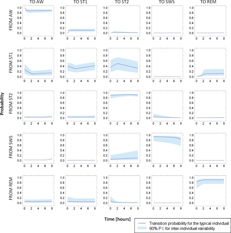
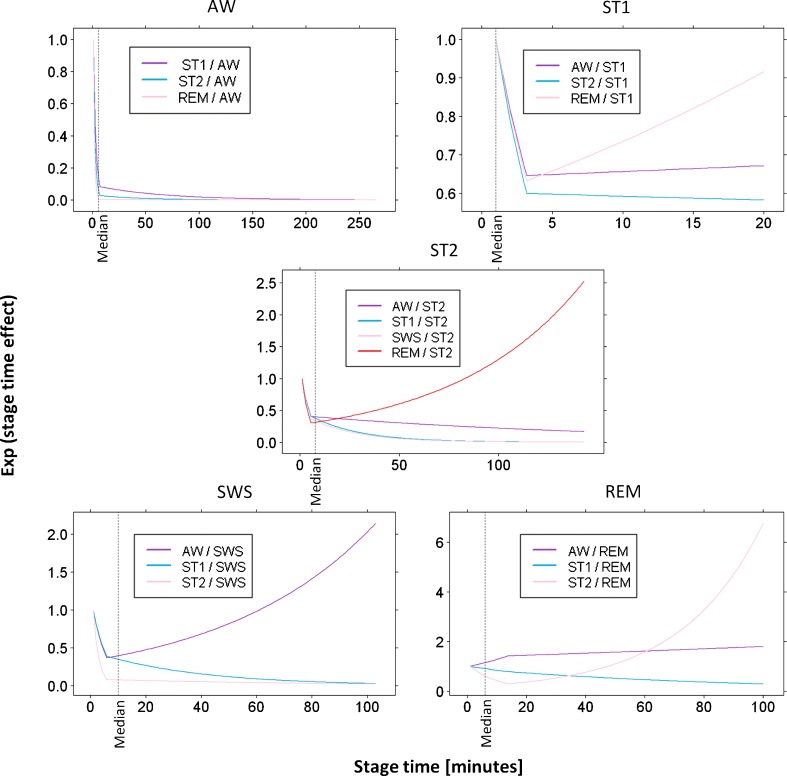
Transition probability profiles were computed from the estimated parameters and are shown in Fig. 1. Estimated stage time effects are shown in Fig. 2.

Fig. 1.

Probability profiles for all the transitions between sleep stages. Their computation is done for the median stage times over the nighttime and the whole patient population

Fig. 2.

Stage time effects estimated in the different sub-models. Exp(stage time effect) is used in order to visualize multiplicative effects on probabilities ratios instead of additive effects on logits (less intuitive). Median stage times over the nighttime and the whole patient population are also reported in each plot

In each sub-model, an important reduction in OFV was achieved, with respect to the base model (7) (see the first three columns of Table III). Most of OFV reduction was due to the introduction of stage time effect: in cases where covariance elements and initial sleeplessness differentiation still had to be introduced, the implementation of stage time effect produced in the sub-models AW, ST2, SWS, ST1, and REM reductions of 5,110, 1,275, 874, 88, and 61 points, respectively. The decrease of OFVs amounted to some tens when introducing the final reference state for the logits (Eq. 6), covariance elements for inter-individual variability (Eq. 10), and initial sleeplessness differentiation for the logits in sub-model AW. Similar outcomes were obtained using BIC. It was not possible to evaluate the effect of fixing one transition probability to zero (in each sub-model, ST2 excluded) with either OFVs or BIC since the few observations for which transitions assumed impossible actually happened had to be removed.

Table III.

OFVs for the Five Sub-models Identified on Study A or B on Different Scenarios

Sub-models	A, Bizzotto et al.	A, final model	A, covariate effects inclusiona	B, parameter values from A	B, after likelihood maximization
AW	26,983	21,662	21,605 (7)	11,627	11,434
ST1	24,264	24,086	24,070 (2)	19,752	19,511
ST2	49,984	48,733	48,705 (3)	33,772	33,441
SWS	9,341	8,380	–	5,299	5,214
REM	14,798	14,687	14,668 (2)	8,906	8,811

^aThe number of included covariate effects is indicated between parenthesis

Internal Validation

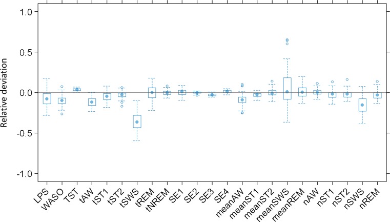
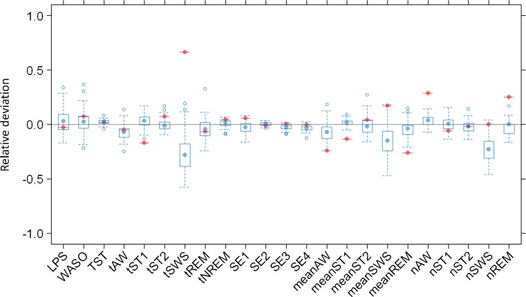
The sPPC outcome for the final model is presented in Fig. 3 and indicates a good agreement between the simulated and the observed efficacy endpoints in most cases. Only 1 out of 23 median aggregated parameters computed from the real study falls outside the range of median values computed from the simulated studies. This parameter is the time spent in SWS (tSWS), which results underpredicted. Other sPPC plots were produced considering statistics different from the median (not reported here), and they corroborate the overall goodness of the model predictive performance in terms of both typical outcomes and variability extent in the population.

Fig. 3.

Results from posterior predictive check: relative deviations of median efficacy endpoints in 100 simulated clinical studies from parameter medians in the real study. Represented parameters are: Latency to persistent sleep (LPS); wake after sleep onset (WASO); total sleep time (TST), time spent in each stage (tAW, tST1, tST2, tSWS, tREM); time spent in non-REM sleep (tNREM); sleep efficiency in 0–2 h of bed time (SE1), 2–4 h of bed time (SE2), 4–6 h of bed time (SE3), and 6–8 h of bed time (SE4); mean extension of each stage (meanAW, meanST1, meanST2, meanSWS, meanREM); and number of transitions to each stage (nAW, nST1, nST2, nSWS, nREM)

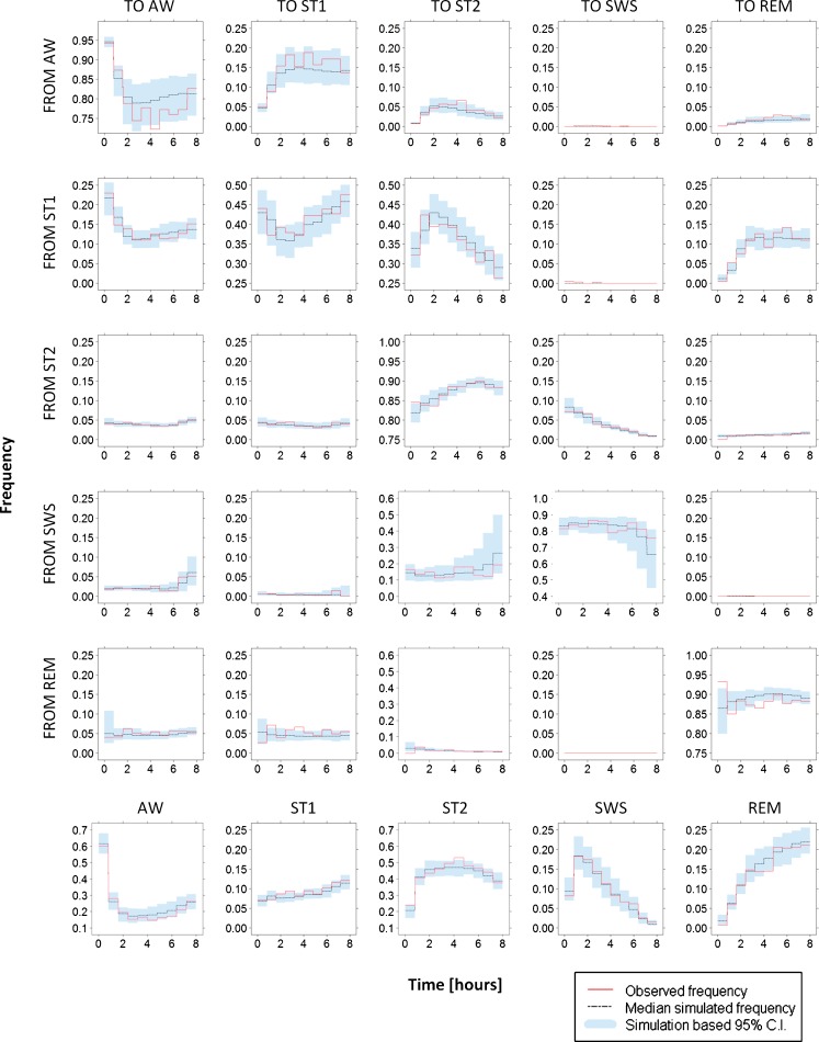
Figure 4 shows the results of VPC implementation on transition frequencies, , and stage frequencies, . The plots show a general very good agreement between the observed and simulated statistics. A slight bias can be detected on transitions from ST2 to REM, from REM to ST2, and from REM to REM, only in the very first period after light off. Simulation-based confidence intervals are generally narrow. The largest ones are observed for transitions from AW to AW and to ST1, from SWS to ST2 and to SWS (especially in the last hours of the night), and from REM to all sleep stages, only in the first hour.

Fig. 4.

Results from visual predictive check on frequency of transitions (first five rows) and stage frequencies (last row). Note that range of the y-axis values is larger in plots at positions (4, 3), (4, 4), (6, 1), and (6, 3)

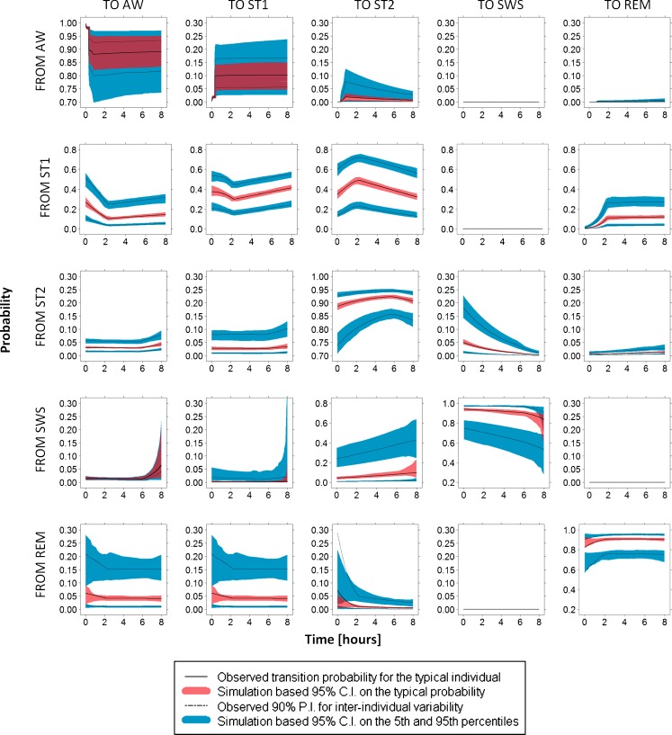
Figure 5 illustrates the results from VEC performed on the time course of transition probabilities. In general, a very good agreement between profiles estimated from raw and simulated data is shown in these plots, with the exception of the transitions from REM to ST2 and from REM to REM at the beginning of the night. Probability confidence intervals on transitions from AW, SWS, and REM are larger compared with the other ones, and they vary according to the amount of available information (depicted in the last row of Fig. 4).

Fig. 5.

Results from visual estimation check on transition probabilities. Note that two different scales are used for the y-axis in the different plots. Note also that dark red areas come from the superimposition of light red and blue confidence intervals (see the typical and 5th and/or 95th confidence intervals for sub-models AW, SWS, and REM)

External Validation

The five final sub-models were successfully identified using dataset B. The last two columns of Table III show the estimated OFVs using parameter values estimated from study A and using parameter values estimated from study B. Distributions of EBEs in the two scenarios are not shown here since η-shrinkage (21) was high in most occasions (>25%).

Final parameter estimates from study B are shown in ESM Table II. They were used to compute typical probability profiles along nighttime, at stage time = 1 epoch, and at median stage time. These profiles are not shown here as only few small differences could be found in comparison with previously computed profiles. When using dataset B, variance estimates for inter-individual variability were instead strongly reduced: averages of variances on the logits were reduced by 75%, 39%, 34%, 24%, and 18% in sub-models SWS, ST1, REM, AW, and ST2, respectively.

sPPC on median aggregated parameters from the new study is visualized in Fig. 6. The performance looks very similar to the one shown in Fig. 3 on data from study A. WASO, tAW, and tSWS are even slightly better predicted. The simultaneous comparison with median efficacy endpoints computed from dataset A (Fig. 6, purple dots) highlights a reduced predictive performance for the aggregated parameters which are highly variable in the two studies (see tST1, tSWS, meanAW, meanSWS, and nREM).

Fig. 6.

Results from posterior predictive check on dataset B: median aggregated parameters computed on dataset B are compared with the corresponding median aggregated parameters computed on 100 datasets simulated from parameter values estimated on dataset B. Comparison is shown in terms of relative deviation. Represented parameters are described in Fig. 3 legend. Red dots are depicted for visualizing the relative deviation of median values computed from study A, from median values computed from study B

Covariate Selection

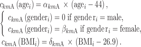
Stepwise covariate modeling brought to OFV reduction in all sub-models, SWS excluded, as indicated in the fourth column of Table III. All of the three analyzed covariates (age, gender, and BMI) were included, linearly affecting various model parameters in different night sections. Thus, the vector of individual logits at the nighttime break points (Eq. 11) becomes a function of both t_s and the covariate values = [age_i, gender_i, BMI_i]^T for the subject i:

13

In the last equation, one has

14

and

15

, , and are equal to zero if the covariate effect is not significant; the median values for age and BMI in the population are 44 and 26.9. During initial sleeplessness, the expression used in Eq. 13 becomes the following:

16

Equations 14 and 15 can be rewritten for break points BPB, BPC, BP1, BP2, and BP3 similarly.

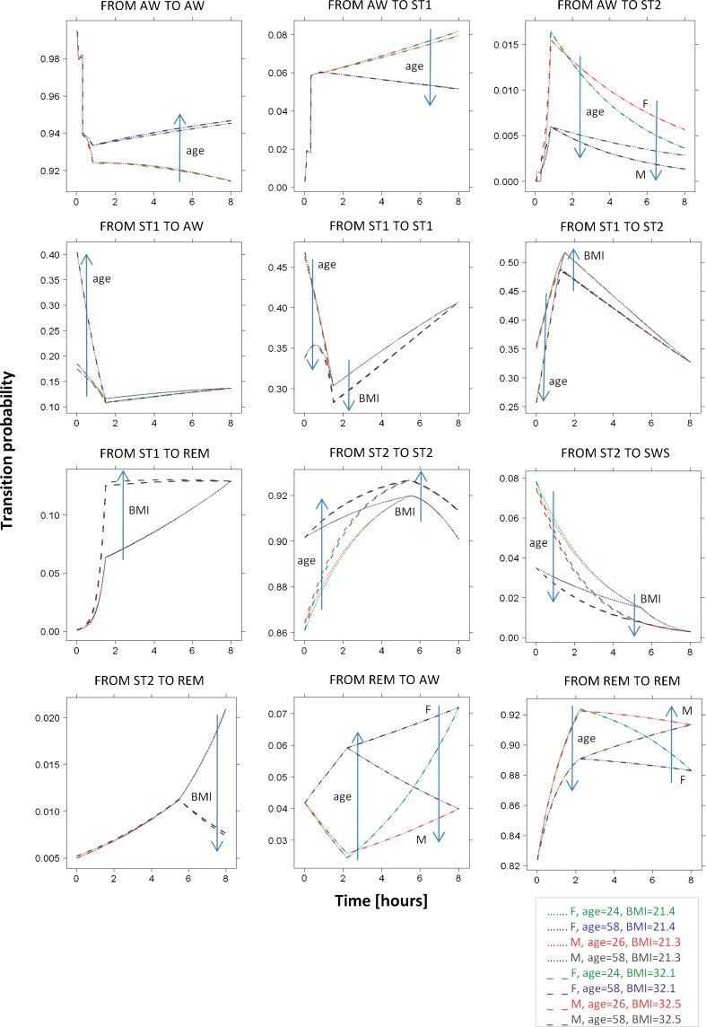
A visual representation of the selected covariate effects is provided by Fig. 7, where typical individual probability profiles are shown for different covariate values. A reduction in inter-individual variability was generally not achieved. The application of sPPC to the obtained full model did not show any relevant improvement in the model performance.

Fig. 7.

Covariate effects on the typical individual profiles of some transition probabilities. The computation of probability values is done for covariate values chosen as follows: in both the male and female populations of study A, the 5th and 95th percentiles for age and BMI values are computed and used in each of their four combinations. Stage times and length of initial sleeplessness are chosen as the median values in the whole population. Effects are shown only on the transitions for which maximum changes in the probability values using the four combinations are >0.01

DISCUSSION

This work was performed to (1) develop a Markov chain model to describe transitions between sleep stages through multinomial logistic functions and combine the best features of similar models available in the literature; (2) validate the new implementation by means of partly new diagnostic methods; and, finally, (3) analyze the effects of covariates as age, gender, and BMI on the parameters of the final model. The model development strategy was aimed to improve the model’s predictive performance while preserving model simplicity, in accordance with the principle of parsimony. The latter was instrumental in developing second-stage models accounting for covariates and drug effect.

The structure of the final Markov chain model was taken from Bizzotto et al. (7). The major change adopted during the model development process was the introduction of stage time (time elapsed since the last change in sleep stage) as a predictor of logit values, in addition to nighttime. Its multiplicative effects on ratios of transition probabilities were found to change greatly during stage time so that the sensitivity of the logits to stage time was comparable or even higher than the sensitivity to nighttime. For this reason, the degrees of freedom in the parameterization of the relationship between logit functions and nighttime could be set as equal to the degrees of freedom in the relationship with stage time (break point numbers in piecewise linear functions of nighttime lowered from 6 to 3). And, for the same reason, it would be interesting to test whether the inclusion of inter-individual variability and covariate effects can significantly modify the individual profiles of stage time effects, besides the individual profiles of nighttime effects.

The choice to select the sleep stage recorded at epoch t − 1 as the reference stage in the definition of logits at epoch t allowed an easy interpretation of plots of stage time effects vs. stage time: increasing values in the profiles indicate higher probability to exit from the current sleep stage, and vice versa. These profiles resulted to be approximately L-shaped in many cases, meaning that transitions to new states happen with higher probability in the first minutes than later on. However, high early transition probabilities may be partially related to sleep scoring difficulties when sleep stages are changing (5). As exceptions to the “L-shape rule,” there are transitions which become likely again (U-shaped) when stage time reaches high values: this is the case for transitions from ST1 and ST2 to REM, from SWS to AW, and from REM to ST2.

Since it was shown that median ST1 time (1 epoch only) anticipates the decline in ST1 time effect and that ST1 is the stage with a higher probability of transitioning to other stages during nighttime, it can be claimed that stage 1 sleep is a state of “fast transition” toward other more stable sleep states (22). Another way to explain this is thinking that the separation of the physiological stages of sleep in five states (AW, ST1, ST2, SWS, and REM) is the discretization of a continuum done with some degree of grossness. SWS, for example, is already explicitly used as a state in which the characteristics of stage 3 sleep and stage 4 sleep are aggregated together (4). Similarly, each of the five labels used for the recorded sleep stages likely aggregates an interval of different characteristics changing on a continuous domain. The recorded sleep stages can be thought of as refractory aggregated states, or as observable discrete states on the top of a layer of hidden continuous (or at least more refined) states. A more refined discretization of sleep states (and of nighttime) would probably make unnecessary the use of stage time effects (i.e., semi-Markov models). According to this hypothesis, the degree of aggregation of underlying more refined states seems lower in ST1 than in other states. The same can be thought about REM sleep since in this case, stage time effect was estimated to be quite flat over stage time. In fact, the removal of the first-order assumption on our Markov chain model was less important for ST1 and REM, as confirmed by the small values of OFV drop in the two sub-models.

Inclusion of stage time effect and of the other features described in “RESULTS” produced an improvement of model predictive performance, as shown by simplified posterior predictive check (sPPC): when comparing the base model (7) and the final model (presented with this paper) in terms of this diagnostic technique, a general refinement of the predictive performance on overall sleep parameters is depicted. The most significant improvements were obtained on latency to persistent sleep (LPS), number of transitions to AW (nAW) and to ST1 (nST1), and time spent in ST1 (tST1). The introduction of specific parameters for initial sleeplessness was particularly important for the improvement on LPS. Incidentally, initial sleeplessness can be thought of as a sixth sleep stage (6), which cannot be observed after the first epoch of sleep occurs (the AW state, instead, can be seen thereafter).

As part of model development, significant correlations between logits from a specific sleep stage have also been investigated: the results highlight that diagonal variance–covariance matrices are not optimal in sub-models where the probability of staying in a state is not clearly dominating on the probabilities of transitioning to other states. Moreover, correlations between individual logits of sub-models ST2 and SWS were tested since aggregated sleep parameters related to SWS were predicted with some bias (see sPPC). No improvements were obtained when including such correlations, but the bias could be justified as well, as specified later in the next paragraph.

The Markov chain model was internally validated through three complementary visual diagnostics on categorical data. sPPC assessed the model’s capability in predicting overall sleep parameters (usually considered as efficacy endpoints in clinical studies) close to the observed ones. Visual predictive check (VPC) focused on the accuracy of sleep description along the independent variable (nighttime tested here, stage time was not considered): since data were categorical, stage frequencies and transition frequencies, and the uncertainty on their prediction, were considered. Visual estimation check (VEC) was introduced in this work as a new tool able to validate the capability of estimating accurate and precise model parameters through a graphic description of accuracy and precision on transition probability time courses. The name “visual estimation check” was chosen because the effect (during nighttime) of possible weaknesses in the estimation method can be visually checked, even if not easily distinguished from the effects of potential model misspecifications; however, the simultaneous use of VPC and VEC is recommended to overcome this kind of issue. sPPC, VPC, and VEC showed that the employed model slightly suffers in a couple of scenarios: statistics with high variability despite similar sleep patterns were predicted with some bias (see, for example, the aggregated sleep parameters related to SWS); small amount of observations for a specific sleep stage determined small bias (if in the Markov chain departure) or inflated uncertainty in the VPC and VEC outcomes. Since outcomes from VPC and VEC were mostly similar, it can be claimed that slight bias and uncertainty in VEC were mostly due to the imperfection of the model’s structure rather than the estimation of its parameter values. Therefore, despite the slight bias just mentioned, the three diagnostic tools showed an overall good performance of the developed Markov chain model in describing the data and of the employed estimation technique. The maximum likelihood estimator, with Laplacian approximation as implemented in NONMEM VI, was shown in the literature to suffer in the case of high η-shrinkage (23). In our case, despite 3 out of 15 values of η-shrinkage being >25%, it revealed instead to be robust.

The Markov chain model has also been validated on a dataset (from study B) which was not used in model development. The validation dataset included less subjects (81 vs. 116) whose characteristics were similar to those of the original dataset (from study A). Ten subjects from study B would have been excluded from study A according to its inclusion criteria: these subjects would not have been severe enough since their TST and LPS values were roughly 5 min above and 5 min below, respectively, compared with the inclusion criteria of study A. Nevertheless, it was shown in “RESULTS” that the proposed model could adequately describe also the new data: the parameters estimated in the two datasets were similar, and the OFVs differed of maximum 300 when using study B with parameter estimates from likelihood maximization on study A or on study B. The new final parameter estimates for the typical individual were used to compute typical probability profiles along nighttime (plots not shown). Few typical probabilities of staying in the different sleep stages were just slightly different compared with the corresponding probabilities estimated from the original dataset: (a) transitioning from AW to ST1 was slightly more likely, at about 1–2 h from light off and short AW stage time; (b) moving from ST1 to ST2 was less likely during all nighttime; (c) transitioning from ST2 to AW was more likely, in the last hour before light on; and (d) moving from SWS to ST2 was more likely during all night, at low SWS stage time. The last difference likely impacts on the lower time spent in SWS (tSWS) and mean extension of SWS (meanSWS), detected through sPPC.

Age, gender, and BMI were found to be statistically significant predictors of transition probability profiles during nighttime in the considered population of insomniac subjects under placebo. However, the predictive performance of the model and the explanation of inter-individual variability were not improved by their inclusion. Each covariate significantly influenced specific transitions, in specific nighttime intervals; therefore, the multiple covariate effects could be diluted if evaluated on aggregated sleep parameters. The choice of the covariate–parameter relations to include or exclude in the model was based on p values which need to be interpreted with caution since multiple comparisons are involved (24).

To our knowledge, this is the first analysis where age, BMI, and gender are considered potential covariates with respect to transitions between sleep stages. Moreover, transitions are considered here in terms of transition probabilities rather than transition frequencies. In addition, the nature of this model allows understanding in which part of nighttime the effect is significant. Probability was found to increase with age for transitions to AW and to decrease for transitions to ST2 and SWS, in the first hours; it was found to increase for the transition from REM to AW, during intermediate hours; and it was found to increase for transitions to AW, in the last hours. These effects are consistent with previous findings from the literature (9–12), described in terms of sleep stage percentages, arousal index, sleep efficiency, total sleep time, and time spent awake after falling asleep. Gender was found to affect transition probabilities only in the last part of the night: transitions from AW to ST2 and from REM to AW appeared more likely in women. In the literature, it has been reported that females have higher sleep efficiency, higher SWS percentage, and lower light sleep (ST1 and ST2) percentage (9) compared with males. Therefore, in this case, linking our findings with previous ones becomes challenging. Finally, high BMI values translated into less likely transitions from ST1 to ST2, ST1 to REM, and ST2 to SWS, in the intermediate night hours, and from ST2 to REM, in the last hours. These effects are compatible with lower SWS percentage (13,14), arousal index (9), and sleep duration (14,15) reported in the literature.

It is important to notice that the covariate analysis was performed on insomniac subjects treated with placebo. Although the considered covariates did not appear to be relevant in terms of model predictive performance when including or excluding their effects, their relevance cannot be excluded in a patient population with a wider range of severity. In fact, it is likely that the effect of age, gender, and BMI on sleep architecture is highly masked by the insomnia severity. Further applications of this model in different patient populations or healthy subjects are recommended to better characterize and possibly differentiate physiological and pathophysiological sleep architecture.

Finally, herein, the proposed approach was applied to data from a population of insomniac patients treated with placebo, but it can be easily extended to estimate the effect of drug exposure on the transition probabilities. In this way, the key sleep patterns differentiating the mechanism of action of different hypnotic compounds may be identified. As for stage time effect and covariate effect, drug effect can be added to the definition of the logits in the model. The detection of the logits and the stage time and/or nighttime values on which drug effect is significant can be performed with up-to-date methods for covariate inclusion, similar to what was done in this work for covariate analysis.

CONCLUSIONS

This work proposed multinomial mixed-effect Markov chain models as a robust modeling framework for describing and predicting sleep architecture obtained from PSG. The model structure has been improved with respect to previous models, as shown by both internal and external validation procedures. The set of adopted diagnostics may represent a useful base for future evaluation of models dealing with categorical non-ordered data. Age, gender, and body mass index have been found to influence many features of sleep architecture in insomniac patients. Such influence has been characterized in a second-stage model including statistically significant covariate effects.

Electronic Supplementary Materials

Below is the link to the electronic supplementary material.

Appendix 1

NONMEM model file for sub-model AW:

Appendix 2

Some Lines from the Dataset Used with Sub-model AW (the Whole Dataset Can Be Found as ESM Table II)

ID	TIME	STAG	MDV0	MDV	STT	SL	IS
142	52	0	0	0	51	0	55
142	53	0	0	0	52	0	55
142	54	1	0	0	53	0	55
142	55	1	1	0	1	1	55
142	56	1	1	0	2	1	55
126	343	2	1	0	10	1	71
126	344	2	1	0	11	1	71
126	345	0	1	0	12	1	71
126	346	1	0	0	1	1	71
126	347	0	1	0	1	1	71
126	348	1	0	0	1	1	71
126	349	1	1	0	1	1	71

References

- 1.Mai E, Buysse D. Insomnia: prevalence, impact, pathogenesis, differential diagnosis, and evaluation. Sleep Med Clin. 2008;3(2):167–174. doi: 10.1016/j.jsmc.2008.02.001. [DOI] [PMC free article] [PubMed] [Google Scholar]
- 2.Gimenez S, Clos S, Romero S, Grasa E, Morte A, Barbanoj MJ. Effects of olanzapine, risperidone and haloperidol on sleep after a single oral morning dose in healthy volunteers. Psychopharmacology. 2007;190:507–516. doi: 10.1007/s00213-006-0633-7. [DOI] [PubMed] [Google Scholar]
- 3.Penzel T, Kesper K. Physiology of sleep and dreaming. Sleep Apnea. 2006;35:13–20. doi: 10.1159/000093138. [DOI] [Google Scholar]
- 4.Rechtschaffen A, Kales A. A manual of standardized terminology, techniques and scoring system for sleep stages of human subjects. Washington, DC: Public Health Service, US Government Printing Office; 1968. [Google Scholar]
- 5.Karlsson MO, Schoemaker RC, Kemp B, Cohen AF, van Gerven JMA, Tuk B, et al. A pharmacodynamic Markov mixed-effects model for the effect of temazepam on sleep. Clin Pharmacol Ther. 2000;68:175–188. doi: 10.1067/mcp.2000.108669. [DOI] [PubMed] [Google Scholar]
- 6.Kjellsson MC, Ouellet D, Corrigan B, Karlsson MO. Modeling sleep data for a new drug in development using Markov mixed-effects models. Acta Universitatis Upsaliensis. Digital Comprehensive Summaries of Uppsala Dissertations from the Faculty of Pharmacy 59; 2008. [DOI] [PubMed]
- 7.Bizzotto R, Zamuner S, De Nicolao G, Karlsson MO, Gomeni R. Multinomial logistic estimation of Markov-chain models for modeling sleep architecture in primary insomnia patients. J Pharmacokinet Pharmacodyn. 2010;37:137–155. doi: 10.1007/s10928-009-9148-2. [DOI] [PubMed] [Google Scholar]
- 8.Bergstrand M, Hooker AC, Karlsson MO. Visual predictive checks for censored and categorical data (abstract). 2009. p. 18, Abstr 1604. www.page-meeting.org/?abstract=1604.
- 9.Redline S, Kirchner HL, Quan SF, Gottlieb DJ, Kapur V, Newman A. The effects of age, sex, ethnicity, and sleep-disordered breathing on sleep architecture. Arch Int Med. 2004;164:406–418. doi: 10.1001/archinte.164.4.406. [DOI] [PubMed] [Google Scholar]
- 10.Vitiello MV. Sleep in normal aging. Sleep Med Clin. 2006;1:171–176. doi: 10.1016/j.jsmc.2006.04.007. [DOI] [PMC free article] [PubMed] [Google Scholar]
- 11.Sahlin C, Franklin KA, Stenlund H, Lindberg E. Sleep in women: normal values for sleep stages and position and the effect of age, obesity, sleep apnea, smoking, alcohol and hypertension. Sleep Med. 2009;10:1025–1030. doi: 10.1016/j.sleep.2008.12.008. [DOI] [PubMed] [Google Scholar]
- 12.Van Cauter E, Leproult R, Plat L. Age-related changes in slow wave sleep and REM sleep and relationship with growth hormone and cortisol levels in healthy men. JAMA. 2000;284(7):861–868. doi: 10.1001/jama.284.7.861. [DOI] [PubMed] [Google Scholar]
- 13.Rao MN, Blackwell T, Redline S, Stefanick ML, Ancoli-Israel S, Stone KL. Association between sleep architecture and measures of body composition. Sleep. 2009;32(4):483–490. doi: 10.1093/sleep/32.4.483. [DOI] [PMC free article] [PubMed] [Google Scholar]
- 14.Kohatsu ND, Tsai R, Young T, Van Gilder R, Burmeister LF, Stromquist AM, et al. Sleep duration and body mass index in a rural population. Arch Int Med. 2006;166:1701–1705. doi: 10.1001/archinte.166.16.1701. [DOI] [PubMed] [Google Scholar]
- 15.Van Cauter E, Knutson KL. Sleep and the epidemic of obesity in children and adults. Eur J Endocrinol. 2008;159(Suppl 1):S59–S66. doi: 10.1530/EJE-08-0298. [DOI] [PMC free article] [PubMed] [Google Scholar]
- 16.Beal SL, Sheiner LB. NONMEM user’s guides. San Francisco: NONMEM Project Group; 1998. [Google Scholar]
- 17.Holford N. VPC, the visual predictive check—superiority to standard diagnostic (Rorschach) plots (abstract). 2005; p. 14, Abstr 738. www.page-meeting.org/?abstract=738.
- 18.Jönsson S, Kjellsson MC, Karlsson MO. Estimating bias in population parameters for some models for repeated measures ordinal data using NONMEM and NLMIXED. J Pharmacokinet Pharmacodyn. 2004;31(4):299–320. doi: 10.1023/B:JOPA.0000042738.06821.61. [DOI] [PubMed] [Google Scholar]
- 19.Duval V, Karlsson MO. Impact of omission or replacement of data below the limit of quantification on parameter estimates in a two-compartment model. Pharm Res. 2002;19(12):1835–1840. doi: 10.1023/A:1021441407898. [DOI] [PubMed] [Google Scholar]
- 20.Jonsson EN, Karlsson MO. Automated covariate model building within NON-MEM. Pharm Res. 1998;15:1463–1468. doi: 10.1023/A:1011970125687. [DOI] [PubMed] [Google Scholar]
- 21.Savic RM, Karlsson MO. Importance of shrinkage in empirical Bayes estimates for diagnostics: problems and solutions. AAPS J. 2009;11(3):558–569. doi: 10.1208/s12248-009-9133-0. [DOI] [PMC free article] [PubMed] [Google Scholar]
- 22.Carskadon MA, Dement WC. Normal human sleep: an overview. In: Kryger MH, Roth T, Dement WC, editors. Principles and practice of sleep medicine. Philadelphia: W.B. Saunders; 1989. pp. 3–13. [Google Scholar]
- 23.Kjellsson MC. Methodological studies on models and methods for mixed-effects categorical data analysis. Acta Universitatis Upsaliensis. Digital Comprehensive Summaries of Uppsala Dissertations from the Faculty of Pharmacy 83; 2008.
- 24.Ribbing J, Jonsson EN. Power, selection bias and predictive performance of the population pharmacokinetic covariate model. J Pharmacokinet Pharmacodyn. 2004;31(2):109–134. doi: 10.1023/B:JOPA.0000034404.86036.72. [DOI] [PubMed] [Google Scholar]
Associated Data
This section collects any data citations, data availability statements, or supplementary materials included in this article.
Supplementary Materials
Statistics on age, BMI and gender in study A and B subjects. (DOC 26 kb)
Model parameter values estimated from study B. (DOC 311 kb)