MOLECULAR FACTORS GOVERNING INHIBITION OF ARYLIMIDAMIDES AGAINST LEISHMANIA: CONSERVATIVE COMPUTATIONAL MODELING TO IMPROVE CHEMOTHERAPIES

Abstract

A dataset of 55 compounds with inhibitory activity against L. donovani axenic amastigotes and L. amazonensis intracellular parasites was examined through three-dimensional quantitative structure-activity relationship modeling employing molecular descriptors from both rigid and flexible compound alignments. For training and testing purposes, the compounds were divided into two datasets of 45 and 10 compounds, respectively. Statistically significant models were constructed and validated via the internal and external predictions. For all models employing steric, electrostatic, hydrophobic, H-donor and H-acceptor molecular descriptors, the R² values were greater than 0.90 and the SEE values were less than 0.22. The models obtained from rigid and flexible compounds were employed together to obtain a conservative method for predictions. This method minimized under predictions. Molecular descriptors from the models were then extrapolated, for the overall predictive devices and the individual compounds, and examined with regard to inhibitory activity. Information gained from the molecular descriptors is useful in the design of novel compounds. The models obtained can be employed to predict activities of the compounds designed and/or form predictions for compounds that exist and have not yet been examined with biological inhibitory assays.

1. Introduction

Leishmania species cause leishmaniasis, an endemic disease found in tropic and subtropic regions riddled with poverty and neglect.^1–3 This infection is most often in the form of cutaneous leishmaniasis where the result is visible skin sores, or visceral leishmaniasis which affects the liver and spleen. Leishmaniasis is primarily transported through the bite of a female phlebotomine sandfly and millions of new cases are reported annually; although, the number of reported cases is probably much lower that the number of actual cases (http://www.who.int/leishmaniasis/burden/magnitude/burden_magnitude/en/print.html).

An estimated half million cases of visceral leishmaniasis occur worldwide annually, and symptomatic infection usually ends in death in the absence of treatment (http://www.who.int/leishmaniasis/visceral_leishmaniasis/en/index.html). Similar to most parasitic diseases plaguing developing countries, there is a lack of affordable and effective therapeutics for leishmaniasis. Traditional treatment of this disease is with pentavalent antimonials such as sodium stibogluconate and meglumine antimoniate, but resistance to antimonials has become a serious problem in India.⁴ The current preferred therapeutics include liposomal amphotericin B (AmBisome), paromomycin, and miltefosine. Single dose AmBisome has shown outstanding efficacy in treating visceral leishmaniasis in India but must be given by injection and is relatively costly.⁵ Paromomycin is effective against visceral leishmaniasis in India and is relatively inexpensive, but optimal treatment requires twenty-one daily injections of this drug.⁶ Miltefosine is effective when given orally for the treatment of Indian visceral leishmaniasis, but the drug is teratogenic, is more expensive than paromomycin, and is prone to the development of resistance.^7–8 In East Africa, antimonial regimens remain the first-line treatment for visceral disease.⁹ Combination therapy has also been implemented in the last few years for the treatment of visceral leishmaniasis to reduce treatment duration, total drug doses, and toxic effects.^9–10 This treatment method also reduces the development of resistance against the drugs and is cost effective.⁷

While not lethal, cutaneous leishmaniasis is a serious problem in developing countries; this infection can lead to severe disfiguring skin lesions when untreated.¹¹ The infection is also most often treated with pentavalent antimonials although liposomal amphotericin B has recently been shown to be effective in the treatment of cutaneous leishmaniasis.^12–12 Pentamidine is used to treat L. guyanensis infections¹³ but not cutaneous infections caused by other Leishmania species. Several other drugs for cutaneous leishmaniasis have been proposed, including allopurinol¹⁴, rifampicin¹⁵, dapsone¹⁶, chloroquine¹⁷, and nifurtimox¹⁸.

Through several research endeavors, activities and toxicities of series of compounds have been gathered and such data have been implemented in rational drug design.^19–22 These studies employ biological data of natural and/or synthetic compounds and computational tools to examine compounds with activity against Leishmania species. Examination of such compounds has led to the formation of predictive models and from these models the importance of some molecular structures has been ascertained. Although specific receptor interaction studies are important, especially when studying mechanisms, intact parasite studies of inhibition and toxicity are crucial for identifying compounds that will eradicate the parasite from hosts.²³ Such studies of synthetic chalcones and phospholipids display effective antileishmanial activity for compounds with: (1) a long alkyl chain, (2) bulky groups at the ends of the alkyl chains, and (3) an electron deficient group.^20,24

Our studies examine a biological dataset of synthetic arylimidamides which possess activities against L. donovani axenic amastigotes and L. amazonensis intracellular parasites. Inhibitory data, in the form of IC₅₀ values, and Comparative Molecular Field Analysis (CoMFA) and Comparative Molecular Similarity Indices Analysis (CoMSIA) molecular descriptors were employed with partial least squares (PLS) regression to correlate the biological data with molecular structures and properties. Predictive models and molecular descriptor potentials derived from the models contribute to the identification and understanding of important molecular features that govern the inhibitory actives of arylimidamides against species of Leishmania.

2. Materials and Methods

Inhibitory data was gathered for arylimidamides with activity against L. donovani axenic amastigotes and L. amazonensis intracellular parasites. This data was implemented for three-dimensional QSAR modeling employing rigid and pharmacophore alignments. The compounds acquired for this study are from the David Boykin compound library at Georgia State University, and representative synthetic procedures are found in the literature.^25–30 The synthesis of many of the compounds used in this study have been reported^29,30 and the remainder were prepared using the same methodology. All compounds were characterized by 1H and 13C NMR and by giving satisfactory elemental analysis (C,H,N within ± 0.4% of theory). The toxicities of some of the most active arylimidamides have been examined through in vitro and in vivo assays, and the data demonstrate that arylimidamides are promicing preclinical candidates for the treatment of visceral leishmaniasis.³⁰

2.1. Inhibition Data

Briefly, IC₅₀ (μM) values were determined for compounds of interest using two assays. The first assay screened against axenic amastigote-like L. donovani, while the second screened against L. amazonensis intracellular parasites. Screening against L. donovani was conducted by: (1) culturing Ld1s parasites in potassium-based medium at pH 5.5, 37 °C, (2) incubating for three days with compounds in a 96-well plate, and (3) adding tetrazolium dye and quantifying the assay spectrophotometrically as outlined previously.²⁹ Evaluation of compounds against L. amazonensis intracellular parasites was conducted by: (1) plating macrophages and allowing the host cells to adhere overnight, (2) adding L. amazonensis promastigotes transfected with the β-lactamase gene (MOI: 5:1) and incubating overnight, (3) adding compounds of interest and incubating for 72 hours at 34 °C, (4) adding nitrocefin in lysis buffer and incubating an additional 3 to 5 hours, and (5) reading the plate at 490 nm as described earlier.^31–32 Experimental IC₅₀ values for L. donovani axenic amastigotes and L. amazonensis intracellular parasites were obtained for 55 compounds.

2.2. Preparation of Compounds for Computational Studies

SYBYL 8.1³³ software was employed to construct all compounds in three-dimensional space. Compounds were then divided into training and testing datasets. These datasets consisted of 45 and 10 compounds, respectively. The compounds of the training dataset then underwent a short molecular dynamics simulation of 1 ns. This system employed SYBYL 8.1 default settings at a constant temperature and volume (NTV). Briefly, (1) the system temperature was set at 300 K with a coupling constant of 100 fs, (2) Maxwell-Boltzmann distribution was employed for initial atom velocities, (3) the non-bonded pair list was updated every 25 fs, and (4) the duration of the molecular dynamics simulations in vacuo was 1 ns with a time step of 100 fs and a snapshot every 1000 fs. The dynamics snapshots displayed several low energy structures. Torsional angles of all training dataset compounds were modified to explore the low energy conformations and modified structures were minimized to convergence using the Tripos force field, conjugate gradient algorithm, and Gasteiger-Hückel charges. The termination gradient was 0.01 kcal/(mol Å) and the maximum iterations were 10⁴.

2.3. Rigid Alignment of Compounds and Resulting Models

Each training dataset of compounds with modified torsional angles was aligned using the “Align Database” option of the QSAR module in SYBYL. CoMFA (steric and electrostatic) and CoMSIA (steric, electrostatic, hydrophobic, H-donors and H-acceptors) molecular descriptors were calculated for the aligned structures and PLS regression was employed to correlate the molecular descriptors of compounds to experimental average IC₅₀ values. The number of components was determined by the smallest predicted error sum of squares. Optimum models employing CoMFA molecular descriptors consisted of three components, whereas the ones with CoMSIA molecular descriptors employed six.

2.4. Flexible Alignment of Compounds and Resulting Models

Five compounds with low IC₅₀ values in the L. amazonensis intracellular parasite assay were employed for flexible compound alignment using the “Align Pharmacophore” option of the GALAHAD module. Parameters were acquired through the “Suggest from Data” option and the best 20 models were collected. The highest scoring model with respect to maximized pharmacophore consensus, maximized steric consensus, and minimized energy was employed as a template for individual compound alignment of the entire training dataset. The “Align Molecules to Template Individually” option was selected and parameters were acquired once more through the “Suggest from Data” option; the “Keep Best N Models” option was reset to 20. Molecular descriptors were calculated for the highest scoring model and PLS regression was implemented in the same manner as for the rigid compounds. The optimum numbers of components were determined as previously described; models with CoMFA molecular descriptors consisted of three components, whereas models with CoMSIA molecular descriptors employed six.

2.5. Statistical Analyses

The statistics calculated1 from PLS regression included: a leave-one-out cross-validated correlation coefficient (Q²), the coefficient of determination (R²), the standard error of estimate (SEE), the F statistic, a bootstrap R² (R²_bs), and a bootstrap SEE (SEE_bs). The bootstrap analysis was used to check the stability of the models through cross-validation into two, five, and ten groups. The average values of the bootstrap analysis are displayed with the rest of the statistics. A scramble test was also preformed to address chance correlation; statistics and predictions are reported in Supplemental Tables S2 and S3.

2.6. Testing Datasets and the Conservative Model Method

The models constructed from the rigid and flexible alignments were employed to examine testing datasets that were aligned via rigid and flexible methods. Of the pIC₅₀ values predicted, for both training and testing datasets, the more negative pIC₅₀ prediction was considered the most viable. This method favors over prediction, larger IC₅₀ values, rather than under prediction.

2.7. Molecular Descriptor Potentials

Molecular descriptor potentials acquired through the mapping of the product standard deviation with respect to molecular descriptor values and coefficients at each lattice point were extrapolated from the models. Default levels of contour by contribution were employed to gather favored and disfavored potentials for overall models. The individual compounds of the models were analyzed via the contour by actual analysis method. Software output was used to determine the proper ranges of assigned favored and disfavored contour regions for individual compounds.

3. Results

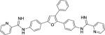
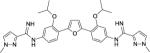
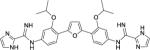
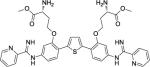
The entirety of the dataset, 45 training and 10 testing compounds (Supplemental Table S1 and Table 3), can be represented via the scaffold structure displayed in Figure 1. At each of the five positions labeled in this figure there are differing atoms or groups: positions one and four display single atom changes in the form of carbon, oxygen, sulfur, and nitrogen, whereas positions two, three and five display larger group substituent modifications as shown in Supplemental Table S1 and Table 3.

Table 3.

Predictions in terms of IC₅₀. Experimental values for compound inhibitory activity against L. donovani axenic amastigotes (LD) and L. amazonensis intracellular parasites (LA) are displayed in columns LD Exp and LA Exp. The predicted values are those from the conservative predictions, LD Calc and LA Calc. These are also displayed in Figure 6.

Name	Structure	LA Exp (μM)	LA Calc (μM)	LD Exp (μM)	LD Calc (μM)
DB710		0.16 ± 0.04	1.4	0.84 ± 0.2	4.0
DB712		0.56 ± 0.08	0.65	2.0 ± 0.6	4.6
DB749		3.1 ± 0.7	1.4	>50	50
DB874		1.4 ± 0.3	0.66	4.2 ± 1.3	3.2
DB889		0.11 ± 0.02	2.3	1.7 ± 0.5	10
DB1856		0.74 ± 0.3	3.2	5.8 ± 0.7	10
DB1857		0.37 ± 0.2	0.69	1.0 ± 0.2	10
DB1864		>10	9.3	5.6 ± 1.8	16
DB1908		>10	4.7	14 ± 1	16
DB1930		5.5 ± 0.2	9.3	>100	63

Figure 1.

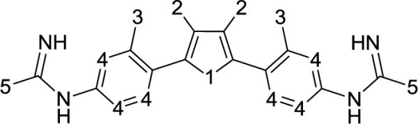
Scaffold structure for compounds with biological inhibitory data for L. donovani axenic amastigotes and L. amazonensis intracellular parasites. The numbered positions on the scaffold identify the locations where compounds differ, and these serve as a guide for explanation of model findings. All training dataset structures and respective inhibitory data can be viewed in Supplemental Table 3 (Appendix). There is an overall plus one charge on these compounds; protonation takes place on the N-C=N groups between the aromatic rings with labeled position 4 and the groups at position 5.

Biological IC₅₀ values were determined for each compound of the training and testing datasets through two assays targeting L. donovani axenic amastigotes and L. amazonensis intracellular parasites. These inhibitory values were averaged and standard errors (n ≥ 3) were calculated (Table 3). For modeling purposes, the IC₅₀ values were log transformed into pIC₅₀ values (pIC₅₀ = −log(IC₅₀)). Figure 2 displays the pIC₅₀ data; experimental values against the L. donovani axenic amastigotes are shown in green, whereas the values against the L. amazonensis intracellular parasites are displayed in blue. The standard error of the data is represented in general by trend lines and the averaged values are shown as triangles and squares, respectively. Notice that the slopes are very similar with values between 0.96 and 1.0, and R² values are 0.95 or higher. This displays the relative range of inhibitory activity and the standard error from the average inhibitory values associated with each synthetic compound in the training and testing datasets. The pIC₅₀ distribution of data is also shown in this figure; the inhibitory activity of arylimidamides against L. donovani axenic amastigotes ranges between approximately −2.5 and 0.5, whereas those active against L. amazonensis intracellular parasites range between about −1.5 and 1.5.

Figure 2.

Biological pIC₅₀ data of synthetic arylimidamides active against L. donovani axenic amastigotes (green) and L. amazonensis intracellular parasites (blue). The negative log values of average experimentally obtained IC₅₀ data, displayed in Supplemental Table 3 (Appendix B) and Table 3, and these values plus and minus respective standard deviations are all plotted against the negative log value of average experimentally obtained IC₅₀ data.

Compounds examined through biological assays were aligned in three-dimensional conformations using two methods: (1) rigid alignments of compounds were obtained through the implementation of the SYBYL “Align Database” option of the QSAR module, and (2) flexible alignments of compounds were acquired through the use of the “Pharmacophore Alignment” option of the GALAHAD module. Rigid alignments were performed on low energy conformations of compounds. Molecular descriptors were then calculated and PLS regression was employed to construct predictive models from the descriptors and respective biological inhibitory data. The best computational models formed consisted of compounds in their most linear conformation with an overall plus one charge. The plus one value was used, since the arylimidamides have a pKa near 7.

Flexible alignment of compounds employed the five most active compounds against the L. amazonensis intracellular parasites from the training dataset (Figure 3). Figure 4 displays the outcome of pharmacophore simulations that lead to PLS regression models employing flexible compounds. The rotation of the compounds allows for visualization of alignment and positioning of identified feature potentials. The observed features governing structure alignment are: (1) four aromatic rings (cyan); (2) N=C–N groups, two positive nitrogens (red) and a H-donor (magenta); (3) atoms at the one and a two position of Figure 1, two H-acceptor (green); (4) atoms at a five position, a H-donor or H-acceptor (overlaid magenta and green equates to dark green). In the next step all of the training and testing compounds were flexibly aligned to the pharmacophore. These alignments can be viewed in relation to rigid alignments (Figure 5). Rigid compounds were aligned by N=C–N groups. Notice that there is a difference in the spatial relationships of the compounds.

Figure 3.

Five of the most active compounds against L. amazonensis intracellular parasites and L. donovani axenic amastigotes.

Figure 4.

GALAHAD potentials as identified by simulations employing the compounds of Figure 3. The identified features are color coded: cyan, hydrophobes; magenta, donor atoms; green, acceptor atoms; red, positive nitrogens.

Figure 5.

Final training (top) and testing (bottom) datasets: flexible alignments (left) and rigid alignments (right).

Inhibitory activities with structures and properties of the aligned compounds were employed to construct predictive models through PLS regression methods. The statistics for these models indicate that CoMSIA molecular descriptors outperform those of CoMFA molecular descriptors (Table 1). This is shown in higher Q², R², and F statistics and lower SEE statistics for the models constructed with rigid compounds. Models from flexible compounds displayed higher R² and F statistics and lower SEE statistics but lower Q² values. The lower Q² are attributed to: (1) torsional variability, (2) differences in optimal low energy structural conformations, and (3) contributions of compound inhibitory activities.³⁴

Table 1.

Statistics of partial least squares predictive models for a biological dataset of synthetic arylimidamides with activities against L. donovani axenic amastigotes (LD) and L. amazonensis intracellular parasites (LA).

	Rigid Alignment				Flexible Alignment
	CoMFA CoMSIA				CoMFA CoMSIA
	LA	LD	LA	LD	LA	LD	LA	LD
Q2	0.23	0.25	0.47	0.59	0.16	0.60	0.07	0.22
SEE	0.45	0.41	0.25	0.18	0.24	0.33	0.16	0.14
R2	0.68	0.77	0.91	0.96	0.91	0.85	0.96	0.97
F	29.1	44.5	61.4	137	131	78.0	159	229
SEEbs	0.35	0.37	0.21	0.16	0.21	0.26	0.12	0.12
R2bs	0.80	0.82	0.94	0.97	0.93	0.90	0.98	0.98

The internal (training dataset) and external (testing dataset) predictions of the models are displayed in Figure 6 where predicted pIC₅₀ values are plotted versus the experimental pIC₅₀ values. The training dataset of this figure is colored in accordance to Figure 2, whereas all testing dataset predictions are in red. Although internal predictions were linear, some testing dataset compounds were more difficult to predict for than others. The variance in compound prediction differed between the models for compounds of rigid and flexible alignments; hence, by taking the most negative prediction of each compound regardless of rigid or flexible alignment and plotting these values against respective experimental data a conservative method for prediction can be obtained. The combination of the models reduces under prediction. Table 3 displays the testing dataset along with experimental average IC₅₀ values, plus or minus respective standard error, along with the conservative model IC₅₀ prediction. The R²_Test and SEE_Test values for the experimental and predicted conservative data shown in Table 3 are respectively 0.36 and 0.23 for L. amazonensis intracellular parasites, and 0.72 and 0.20 for L. donovani axenic amastigotes; the statistics are calculated on the pIC₅₀ data. When the R² _Test statistics are calculated on the IC₅₀ data of Table 3 the R² Test statistics are 0.59 and 0.93. The statistics give a rough idea of model predictability, whereas the actual prediction in relation to experimental data shows the model's true ability to predict with relation to standard error.

Figure 6.

Internal (blue and green) and external (red) predictions. The internal predictions are those for the training compounds and external predictions are for the testing dataset of compounds. The L. amazonensis experimental versus predicted results are shown in blue (left) and those for L. donovani in green (right). The experimental versus predicted results from top to bottom are predictions from implementing rigid (top) and flexible (center) compounds. The conservative predictions (bottom) are essentially the more negative of the two pIC₅₀ predictions resulting from the models with rigid and flexible compounds. Since the scale observed is the negative log of the IC₅₀, this method reduces under prediction.

From the models employing CoMSIA, three-dimensional molecular descriptor potentials were determined and viewed as surfaces in relation to the overall models (Figure 7 and Supplemental Figure S1) as well as individual compounds (Figure 8 and Supplemental Figure S2). Figure 7 displays the overall CoMSIA molecular descriptors for the rigid and flexible models. It is evident that each overall model displays different molecular descriptor potential contributions for the steric, electrostatic, hydrophobic, H-donor and H-acceptor potentials. This indicates that each model is constructed somewhat differently; although there are similarities between the results obtained. Using the positions of Figure 1 as a reference: (1) steric bulk is favored (green) at positions three and five and perhaps not symmetrically, whereas disfavored steric bulk (yellow) regions are just outside those favored, (2) positive electrostatic charge is favored (blue) at one, if not both, of the N=C–N groups near position five, whereas negative charge is favored (red) predominantly at or near position one and outside one of the N=C–N groups, (3) hydrophobic interactions are favored (yellow) at positions two and five, whereas disfavored hydrophobic interactions (gray) are near positions three and outside positions five, (4) H-donor atoms are favored (cyan) predominantly at or below the five position and disfavored (purple) in areas beyond favored regions, and (5) H-acceptors are favored (magenta) near the terminal N=C–N groups, and disfavored (red) below the four position(s) and outside favored N=C–N groups of the comparison molecule DB766.

Figure 7.

Overall models with CoMSIA molecular descriptor surfaces for both rigid and flexible structure alignments of compounds active against L. amazonensis; DB766 is displayed as a reference compound. Favored potentials from steric to H-acceptor molecular descriptors are green, blue, yellow, cyan, and magenta, whereas disfavored potentials from steric to H-acceptor molecular descriptors are yellow, red, gray, purple, and red. Results for L. donovani can be found in Supplemental Figure S1.

Figure 8.

CoMSIA findings with respect to Figure 1 and molecular descriptor potentials of Figure 7. The favored hydrophobic potentials have been changed to orange to improve visualization and insure that steric potentials were not displayed. The left most column consists of numbers correlated to positions of Figure 1. The column to the right consists of the compounds name. This is followed by the compounds and their respective molecular descriptor potentials for each the final models. To improve compound visibility, the results for only L. amazonensis are shown above. Results for L. donovani can be found in Supplemental Figure S2.

With regard to the scaffold structure of Figure 1, Figure 8 displays the molecular descriptor potentials of individual compounds based on CoMSIA molecular descriptors. The molecular descriptor potential regions of individual molecules appear to be more consistent within their respective rigid and flexible models than they were in the overall models of Figure 7 and Supplemental Figure S1. The molecular potentials that resulted were, however, also fewer, and included favored and disfavored hydrophobic, favored H-donor and favored H-acceptor potentials.

With the models in Figure 8 and biological data in Supplemental Table S1, it is possible to examine not only the molecular descriptor potentials with regard to model contribution but also the contribution of substructures to biological inhibitory activity. To most effectively describe these findings, it is important that comparisons are made to a compound that is active in both datasets. DB766, a potential drug candidate against visceral leishmaniasis,³⁵ was selected for analyses. With respect to Figure 1, the molecular descriptor potentials for DB766 include: (1) favored hydrophobic potentials near the aromatic groups, (2) favored H-donor potentials are displayed below the left side five position (N=C–N group), and (3) favored H-acceptor potentials are on the N=C–N group opposite the side of the favored H-donor and extended to the terminal aromatic ring. The IC₅₀ values for this compound against L. amazonensis intracellular parasites and L. donovani axenic amastigotes are 0.09 and 0.50 μM, respectively. The general structure of DB1867, compared to DB766, differs only by a sulfur atom at position one and with this change the compound becomes more linear and favored hydrophobic interactions are spread to positions one and two (Figure 8). Potentials for favored H-acceptors are near N=C–N groups and the IC₅₀ values are 0.05 and 0.68 μM, respectively. DB946 is the only compound in the training dataset to differ from DB766 at position two; this compound also differs at position three. The methyl groups at position two fill similar special areas as substituents in position three. Favored hydrophobic potentials reside in position two, three, and five locations. This compound's IC₅₀ values are 0.11 and 0.37 μM, respectively. DB667 and DB1876 differ from DB766 at position three. DB667 possesses hydrogen atoms at position three and molecular descriptor potentials similar to those of DB946 (hydrophobic) and DB766 (H-donor and H-acceptor), although the favored hydrophobic potentials span a greater length for DB667. The IC₅₀ values for this compound are 0.53 and 1.6 μM, respectively. DB1876 displays large disfavored hydrophobic molecular descriptor potentials at the three positions. The remaining potentials are favored hydrophobic potentials near the aromatic rings and favored H-donor and H-acceptor potentials near the N=C–N group(s). This compound has IC₅₀ values of 2.1 and 28 μM, respectively. DB1851 differs from DB766 at position four and this change resulted in favored hydrophobic interactions that span more of the molecule than previous compounds discussed with H-donor and H-acceptor potentials similar to those of DB1876. The IC₅₀ values for this compound are poor, greater than 10 and 50 μM, respectively. DB1921, DB1942, and DB1906 all differ from DB766 at the five positions. DB1921 is flanked at the five positions and has different substituents at the three positions. This compound consists of potentials similar to DB1876; however, it is also missing most of the favored hydrophobic and H-acceptor potentials. The IC₅₀ values for this compound are 4.7 and 41 μM, respectively. DB1942 consists of a longer, more flexible ring structure than DB766 and consists of disfavored hydrophobic molecular descriptor potentials primarily at the five positions. Positive hydrophobic potentials are on the inner aromatic rings or the outer rings near the five position, whereas H-donors are favored on one side of an N=C–N group and H-acceptors are favored at both N=C–N group(s). This compound has IC₅₀ values of 0.81 and 3.6 μM, respectively. The five positions of DB1906 consist of more rings than DB766. The molecular descriptor potentials for this compound were similar to those of DB766 (hydrophobic and H-donor) and DB946 (H-acceptor), IC₅₀ values are 0.27 and 1.9 μM, respectively.

4. Discussion

QSAR studies have previously been employed to determine the importance of chalcone and phospholipid molecular structures, and predict activities and toxicities for series of compounds with activity against Leishmania species.^19–22 These studies found that potent antileishmanial activity occurred when compounds possessed a long alkyl chain, bulky groups at the end of the alkyl chain, and an electron deficient group.^20,24 The structures of chalcones and phospholipids are quite different from each other, and these compounds differ substantially from the arylimidamides examined in this study (Supplemental Table S1).

4.1. Pharmacophore Selection

The numbered locations of Figure 1 aid in the explanation of inhibition results displayed in Figure 2 through the interpretation of pharmacophore consensus potentials (Figure 4) and molecular descriptor contribution potentials (Figures 7 and 8). The pharmacophore alignment of Figure 4 is calculated using the compounds of Figure 3. By only employing the most active compounds, the pharmacophore is strictly for compounds of similar structure and activity. The pharmacophore results suggest the importance of aromatic and positively charged N=C–N groups, and these results can be examined with respect to the chalcone and phospholipid results reported previously.^19–22 The aromatic rings of the arylimidamides can be related to the bulky groups, the positively charged N=C–N groups can be related to the electron deficient groups, and the linker between the central aromatic rings can be related to the long alkyl chain. The pharmacophore results show that the linker between the center aromatic rings does not need to be a ring structure.

4.2. Regression Analyses

PLS regression of calculated molecular descriptor potentials and respective biological inhibitory values for both the rigid and flexible alignments of compounds presented in Figure 5 produced statistically significant models. Models employing the CoMSIA molecular descriptors from rigid structure alignment were the only ones with Q² values greater than 0.5 (Table 1). Q² values greater than 0.5 indicate models with predictability better than chance.³³ What we realize from our models, especially those aligned by flexible conformations, is that each compound contributes to the entirety of the model and that the models constructed from molecular descriptors of flexible compounds may be predicting just as well, if not better, than those constructed from molecular descriptors of rigid compounds (Figure 6). The rigid models of Figure 6 produce a greater amount of under prediction than the flexible models. For example, for the rigid model, one of the compounds active against L. donovani has an experimentally determined pIC₅₀ value of −1.7 and a predicted value of 0, these IC₅₀ values are 50 and 1, respectively, whereas for the flexible model the same compound has a predicted pIC₅₀ value of −1.7, the same as the experimental value.

Under prediction is a problem that needs to be addressed since predictive models such as the ones constructed in this study can be employed to scan potential candidates for synthetic drug design. Often synthetic measures are costly and time consuming; hence, it is better to synthesize only compounds expected to have better inhibitory activity. To minimize under prediction, the minimum pIC₅₀ predictions from the rigid or flexible models were plotted against the average experimental values. These data are shown as the conservative predictions of Figure 6. In this column we see that under predictions are no longer occurring for these models, yet there are still over predictions. Over predictions, as long as they are few, are not as problematic since these values are larger and synthesis will most likely result in experimentally determined inhibitory activity better than calculated.

4.3. Molecular Contributions

A previous study focused on synthetic phospholipids that employed CoMSIA molecular descriptors found that steric and hydrophobic interactions governed the model.²⁰ Similarly, our model was governed by hydrophobic interactions; yet, this contribution of molecular descriptor interactions was followed by H-donor, H-acceptor, steric and then electrostatic (Table 2). When the overall CoMSIA potentials for each molecular descriptor are visualized, it is easier to design modifications to the compounds. Figure 7 allows for comparison between the models and overall analyses. It is important to realize that molecular descriptor potentials are unique to each model; hence, no two models are the same. Positive electrostatic potentials indicate the importance of the N=C–N groups, whereas the steric and hydrophobic potentials show the importance of the rings and substituents. To fully understand molecular descriptor contribution in relation to biological inhibitory data, it is important to analyze the potentials of individual compounds, a selected set of which are shown in Figure 8. These potentials display much more consistency than those for the overall models of Figure 7.

Table 2.

Contribution of CoMSIA molecular descriptors for rigid and flexible models employing structures of training dataset compounds and respective biological activities.

	Rigid Alignment		Flexible Alignment
	L. amazonensis	L. donovani	L. amazonensis	L. donovani
Steric	0.15	0.14	0.13	0.13
Electrostatic	0.11	0.08	0.14	0.15
Hydrophobic	0.47	0.43	0.33	0.34
H-Donor	0.15	0.21	0.20	0.21
H-Acceptor	0.12	0.14	0.20	0.17

4.4. Employing Results

An exciting feature of this type of study is that new compounds can be designed by employing the data acquired from the pharmacophore (Figure 4) and extrapolated molecular descriptor potentials (Figures 7 and 8). To do this, the basic pharmacophore must remain intact and the potentials of the overall models and those of individual compounds should be used for guidance. Since the importance of hydrophobic, H-donor and H-acceptor atoms are clearly displayed as essential potentials for the individual compounds in Figure 8, this is a good place to begin. The favored hydrophobic potentials of the four aromatic rings exhibit significance (Figures 7 and 8); and these are also seen as important in the pharmacophore (Figure 4). Hence, it appears imperative that the four rings remain a constant in our initial modeling efforts. H-bond donors appear to be important to regions near the N=C–N groups (Figures 7 and 8). One of the N=C–N groups is shown as essential in the pharmacophore (Figure 4). Likewise, H-bond acceptors appear to be significant to the region including and between the N=C–N groups and the N of the outer most aromatic rings (Figures 7 and 8). One such region was identified in the pharmacophore (Figure 4). Based on these observations, new compounds have been designed and activity predictions have been obtained (Figure 9). The ranges include the smallest and largest prediction obtained via the models constructed of rigid and flexible compound structures. These are interesting new structure types and can initial compound form this set will be synthesized in due course.

Figure 9.

Compounds designed to illustrate use of the pharmacophore data of Figure 4 and the CoMSIA molecular descriptor fields of Figures 7 and 8. The ranges are the smallest and largest predicted values obtained from the models constructed of rigid and flexible compound structures.

5. Conclusion

For this study, a biological dataset of synthetic arylimidamides and their activities against L. donovani axenic amastigotes and L. amazonensis intracellular parasites were employed for pharmacophore and three-dimensional QSAR modeling. The pharmacophore alignment displayed important features, and the three-dimensional QSAR was performed with and without these findings. The data from the models developed are being used to design novel compounds; whereas the models themselves are being implemented to estimate activities for known and designed compounds of interest. In summary, by employing three-dimensional QSAR it is possible to scan for potentially active compounds both efficiently and conservatively through the use of predictive models. The models are used to designed compounds and respective IC₅₀ activities can be predicted.

The abbreviations used are

CoMFA

Comparative Molecular Field Analysis

CoMSIA

Comparative Molecular Similarity Indices Analysis

QSAR

Quantitative Structure-Activity Relationship

PLS

Partial Least Squares

SEE

Standard Error of Estimate

CPDD

Consortium for Parasitic Drug Development

References

- (1).Alvar J, Yactayo S, Bern C. Trends Parasitol. 2006;22:552. doi: 10.1016/j.pt.2006.09.004. [DOI] [PubMed] [Google Scholar]
- (2).Boelaert M, Meheus F, Sanchez A, Singh S, Vanlerberghe V, Picado A, Meessen B, Sundar S. Trop. Med. Int. Health. 2009;14 doi: 10.1111/j.1365-3156.2009.02279.x. [DOI] [PubMed] [Google Scholar]
- (3).Adhikari S, Maskay N, Sharma B. Health Policy Plan. 2009;24:129. doi: 10.1093/heapol/czn052. [DOI] [PubMed] [Google Scholar]
- (4).Sundar S, More D, Singh M, Singh V, Sharma S, Makharia A, Kumar P, Murray H. Clin. Infect. Dis. 2000;31:1104. doi: 10.1086/318121. [DOI] [PubMed] [Google Scholar]
- (5).Sundar S, Chakravarty J, Agarwal D, Rai M, Murray HN. Eng. J. Med. 2010;362:504. doi: 10.1056/NEJMoa0903627. [DOI] [PubMed] [Google Scholar]
- (6).Sundar S, Agrawal N, Arora R, Agarwal D, Rai M, Chakravarty J. Clin. Infect. Dis. 2009;49:914. doi: 10.1086/605438. [DOI] [PubMed] [Google Scholar]
- (7).Meheus F, Balasegaram M, Olliaro P, Sundar S, Rijal S, Faiz M, Boelaert M. PLoS Negl. Trop. Dis. 2010;4:e818. doi: 10.1371/journal.pntd.0000818. [DOI] [PMC free article] [PubMed] [Google Scholar]
- (8).Sundar S, Murray H. Bull. World Health Organ. 2005;83:394. [PMC free article] [PubMed] [Google Scholar]
- (9).Moore E, Lockwood DJ. Glob. Infect. Dis. 2010;2:151. doi: 10.4103/0974-777X.62883. [DOI] [PMC free article] [PubMed] [Google Scholar]
- (10).van Griensven J, Balasegaram M, Meheus F, Alvar J, Lynen L, Boelaert M. Lancet Inf. Dis. 2010;10:184. doi: 10.1016/S1473-3099(10)70011-6. [DOI] [PubMed] [Google Scholar]
- (11).González U, Pinart M, Reveiz L, Rengifo-Pardo M, Tweed J, Macaya A, Alvar J. Clin. Infect. Dis. 2010;51:409. doi: 10.1086/655134. [DOI] [PubMed] [Google Scholar]
- (12).Wortmann G, Zapor M, Ressner R, Fraser S, Hartzell J, Pierson J, Weintrob A, Magill A. Am. J. Trop. Med. Hyg. 2010;83:1028. doi: 10.4269/ajtmh.2010.10-0171. [DOI] [PMC free article] [PubMed] [Google Scholar]
- (13).Blum J, Desjeux P, Schwartz E, Beck B, Hatz CJ. Antimicrob. Chemother. 2004;53:158. doi: 10.1093/jac/dkh058. [DOI] [PubMed] [Google Scholar]
- (14).Mishra J, Saxena A, Singh S. Curr Med Chem. 2007;14:1153. doi: 10.2174/092986707780362862. [DOI] [PubMed] [Google Scholar]
- (15).Mahajan VK, Sharma NL. J Dermatolog Treat. 2007;18:97. doi: 10.1080/09546630601159474. [DOI] [PubMed] [Google Scholar]
- (16).Al-Mutairi N, Alshiltawy M, El Khalawany M, Joshi A, Eassa BI, Manchanda Y, Gomaa S, Darwish I, Rijhwani M. Int J Dermatol. 2009;48:862. doi: 10.1111/j.1365-4632.2008.04010.x. [DOI] [PubMed] [Google Scholar]
- (17).Rosenblatt JE. Mayo Clin Proc. 1999;74:1161. doi: 10.4065/74.11.1161. [DOI] [PubMed] [Google Scholar]
- (18).Nussbaum K, Honek J, Cadmus CM, Efferth T. Curr Med Chem. 2010;17:1594. doi: 10.2174/092986710790979953. [DOI] [PubMed] [Google Scholar]
- (19).Avery MA, Muraleedharan KM, Desai PV, Bandyopadhyaya AK, Furtado MM, Tekwani BL. J Med Chem. 2003;46:4244. doi: 10.1021/jm030181q. [DOI] [PubMed] [Google Scholar]
- (20).Kapou A, Benetis NP, Avlonitis N, Calogeropoulou T, Koufaki M, Scoulica E, Nikolaropoulos SS, Mavromoustakos T. Bioorg Med Chem. 2007;15:1252. doi: 10.1016/j.bmc.2006.11.018. [DOI] [PubMed] [Google Scholar]
- (21).Ryu CK, Lee Y, Park SG, You HJ, Lee RY, Lee SY, Choi S. Bioorg Med Chem. 2008;16:9772. doi: 10.1016/j.bmc.2008.09.062. [DOI] [PubMed] [Google Scholar]
- (22).Sanders JM, Gomez AO, Mao J, Meints GA, Van Brussel EM, Burzynska A, Kafarski P, Gonzalez-Pacanowska D, Oldfield E. J Med Chem. 2003;46:5171. doi: 10.1021/jm0302344. [DOI] [PubMed] [Google Scholar]
- (23).Santos DO, Coutinho CE, Madeira MF, Bottino CG, Vieira RT, Nascimento SB, Bernardino A, Bourguignon SC, Corte-Real S, Pinho RT, Rodrigues CR, Castro HC. Parasitol Res. 2008;103:1. doi: 10.1007/s00436-008-0943-2. [DOI] [PubMed] [Google Scholar]
- (24).Liu M, Wilairat P, Croft SL, Tan AL, Go ML. Bioorg Med Chem. 2003;11:2729. doi: 10.1016/s0968-0896(03)00233-5. [DOI] [PubMed] [Google Scholar]
- (25).Arafa RK, Brun R, Wenzler T, Tanious FA, Wilson WD, Stephens CE, Boykin DW. J Med Chem. 2005;48:5480. doi: 10.1021/jm058190h. [DOI] [PubMed] [Google Scholar]
- (26).Munde M, Lee M, Neidle S, Arafa R, Boykin DW, Liu Y, Bailly C, Wilson WD. J Am Chem Soc. 2007;129:5688. doi: 10.1021/ja069003n. [DOI] [PMC free article] [PubMed] [Google Scholar]
- (27).Stephens CE, Tanious F, Kim S, Wilson WD, Schell WA, Perfect JR, Franzblau SG, Boykin DW. J Med Chem. 2001;44:1741. doi: 10.1021/jm000413a. [DOI] [PubMed] [Google Scholar]
- (28).Wilson WD, Tanious FA, Mathis A, Tevis D, Hall JE, Boykin DW. Biochimie. 2008;90:999. doi: 10.1016/j.biochi.2008.02.017. [DOI] [PMC free article] [PubMed] [Google Scholar]
- (29).Werbovetz KA, Sackett DL, Delfin D, Bhattacharya G, Salem M, Obrzut T, Rattendi D, Bacchi C. Mol Pharmacol. 2003;64:1325. doi: 10.1124/mol.64.6.1325. [DOI] [PubMed] [Google Scholar]
- (30).Wang MZ, Zhu X, Srivastava A, Liu Q, Sweat JM, Pandharkar T, Stephens CE, Riccio E, Parman T, Munde M, Mandal S, Madhubala R, Tidwell RR, Wilson WD, Boykin D, Hall JE, Kyle DE, Werbovetz KA. Antimicrob Agents and Chemother. 2010;54:2507. doi: 10.1128/AAC.00250-10. [DOI] [PMC free article] [PubMed] [Google Scholar]
- (31).Delfin DA, Morgan RE, Zhu X, Werbovetz KA. Bioorg Med Chem. 2009;17:820. doi: 10.1016/j.bmc.2008.11.031. [DOI] [PubMed] [Google Scholar]
- (32).Buckner FS, Wilson AJ. Am J Trop Med Hyg. 2005;72:600. [PubMed] [Google Scholar]
- (33).Tripos Inc.; St. Louis, MO: 2008. [Google Scholar]
- (34).Golbraikh A, Tropsha A. J Mol Graph Model. 2002;20:269. doi: 10.1016/s1093-3263(01)00123-1. [DOI] [PubMed] [Google Scholar]
Associated Data
This section collects any data citations, data availability statements, or supplementary materials included in this article.