Dynamics of the plague–wildlife–human system in Central Asia are controlled by two epidemiological thresholds

Abstract

Plague (caused by the bacterium Yersinia pestis) is a zoonotic reemerging infectious disease with reservoirs in rodent populations worldwide. Using one-half of a century of unique data (1949–1995) from Kazakhstan on plague dynamics, including data on the main rodent host reservoir (great gerbil), main vector (flea), human cases, and external (climate) conditions, we analyze the full ecoepidemiological (bubonic) plague system. We show that two epidemiological threshold quantities play key roles: one threshold relating to the dynamics in the host reservoir, and the second threshold relating to the spillover of the plague bacteria into the human population.

Plague (Yersinia pestis infection) has played a dramatic role in human history and is still endemic throughout large parts of the Central Asian semideserts (1, 2), where the great gerbil (Rhombomys opimus) is a major reservoir host species (3, 4). Here, we combine monitoring data from the PreBalkhash natural plague focus in southeastern Kazakhstan (74–78°E, 44–47°N) (Fig. 1) (5, 6) with cases of human plague. The abundance of great gerbils and their fleas, and the prevalence of wildlife plague were estimated at up to 78 sites in the PreBalkhash each spring (May and June) and fall (September and October) from 1949 to 1995. Fleas (primarily Xenopsylla gerbilli minax) (7, 8) infesting the gerbils are the main plague vector (3). Plague infection is known to persist in the population only when the gerbil density exceeds a threshold (3, 9). Transmission to humans occurs occasionally through either contacting fleas that have fed on an infected animal (either a rodent or a secondary host) or eating or skinning infected animals (1). The records of human plague began in 1904, with most of the cases occurring before 1949, which was when plague monitoring and flea control began (8, 10) in an effort to eliminate human plague outbreaks. The human plague cases are recorded annually and aggregated spatially, whereas the data on the gerbils and their fleas are recorded biannually. Using recently developed statistical modeling techniques (11) (Methods), we here analyze these data to better understand the underlying dynamic structure of the full ecoepidemiological (bubonic) plague system as it is seen in Central Asia. Although full in the sense of containing all elements—abiotic environment, rodent reservoir, fleas, pathogen, and spillover to humans—it cannot, of course, claim to describe each of these elements exhaustively. For some elements, lack of data prohibits a high level of detail. We have attempted to model as comprehensively as data allowed. For other factors, we have taken a pragmatic approach, for example, by using the error term. For instance, secondary reservoir species (12) are not considered explicitly and are accounted for in this way, which is justified by the fact that the great gerbil is considered to be the dominant host species in the plague focus covered within our study area (13). In particular, we seek in this study to evaluate whether there is evidence of thresholds (incorporating a combination of elements of the whole system) and whether there are separate thresholds within and between species.

Fig. 1.

The rodent–flea–plague model for Central Asia (map in A Right). (A) Summary of the analysis of the plague dynamics in rodents and fleas. Note that the joint conditional distribution of the seasonal growth rates, seasonal flea burdens, and change in the infectious-flea forces in year t is multivariate normal with mean 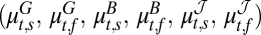, where the superscripts G, B, and refer to the rodent growth rate, flea burden, and change in infectious-flea force models, respectively, and the subscripts s and f refer to the spring and fall seasons, respectively. The model formulation is given in Methods. The plus or minus sign above the parameters refers to a finding of positive or negative effect of the corresponding covariate, respectively. (B Upper) Plot of the rodent growth rate vs. the lag-1.5 flea density during the spring season. (B Lower) Plot of the rodent growth rate vs. the lag-2 flea density during the fall season. The circles correspond to the observed rodent growth rate in each season. The red curves illustrate the mean effect of changes in the lagged flea density (lag-1.5 in the spring and lag-2 in the fall) on the rodent growth rate, with the other covariates fixed at their seasonal mean values. (C Left) The effect of changes in the (log) summer rainfall on the (log) flea burden in the fall season. (C Right) The effect of the (log) summer rainfall on the infectious-flea force in the upper regime of the fall season. Note that the curves illustrate the mean effect of (log) summer precipitation, with other covariates set at their mean values. The unit of rainfall is log-millimeter scale (i.e., the untransformed rainfall data are in millimeters). Open circles are the partial residuals for summer precipitation. The partial residuals are defined as the mean effect of summer precipitation plus Pearson residuals.

Results and Discussion

We investigate the dynamics of rodents together with fleas in the host reservoir through the following three components: abundance of rodents, average number of fleas infecting each rodent (flea burden), and number of free infectious fleas that are searching for a host (infectious-flea force). By modeling these three parameters jointly over time, we seek to understand and predict the persistence and outbreak of plague in the wildlife reservoir and its spillover into the human population. In particular, we observe that the yearly density change in rodents decays exponentially with the flea density (Fig. 1B). The flea burden and infectious-flea force are important in exploring this observed exponential decay in the rodent population. Because plague is unable to invade or persist in the wildlife reservoir unless the density of rodents exceeds a critical threshold (3, 9), the infectious-flea force is assumed to always be zero if the (lagged) density of rodents is below this threshold (estimated in the statistical model). Above the threshold, the infectious-flea force is evaluated as a function of biotic and environmental factors.

In our study area, humans are not fully integrated into the system; however, studying the spillover of plague into humans presents a biomarker for how well plague is controlled in this area. Given the dynamics of plague in the wildlife reservoir, we show that the spillover into humans is best modeled using a threshold model, where the flea density is a key threshold variable that determines when human plague outbreaks may occur. The number of human plague cases is modeled as a function of different sets of biotic and climatic variables depending on whether the flea density is below or above the threshold. Details pertinent to the statistical modeling used for the wildlife reservoir and plague spillover into humans can be found in Methods; estimation techniques, model diagnostics, a bootstrap test justifying the use of the threshold models, and forecasting techniques are all included in SI Text.

We begin by modeling the joint seasonal dynamics of the rodent–flea–plague system, incorporating the annual density change in rodents (referred to as the rodent population growth rate), a measure of the flea burden, and a measure of the infectious-flea force. The rodent population growth rate is defined as G_t = log(R_t/R_{t − 1}), with R_t being the rodent density averaged across all sites at time t (measured every 0.5 y, because samples were taken in spring and autumn). The flea burden is measured by B_t = log(F_t/R_t), where F_t is the flea density averaged across all sites at time t. The infectious-flea force, I_t, is the product of the flea density and the prevalence of plague in rodents (from which fleas become infected) averaged across sites. The change in the infectious-flea force is defined as J_t = log(1 + I_t) − log(1 + I_{t − 1}). The notations used throughout this paper are described and defined in Table S1. The resulting model of the reservoir dynamics that best accounts for the time series of these three variables (Methods has details of its derivation) is summarized in Fig. 1 and Table 1. Candidate explanatory variables are defined in Table S1. The optimum model for the rodent–flea–plague system is a multivariate nonlinear model, where the nonlinearity feature pertains to the behavior of the infectious-flea force as a threshold model with the rodent density being a dominant season-specific variable defining the threshold (SI Text). This result suggests that the rodent population 1.5–2 y earlier has to be sufficiently high for an outbreak to occur, which is consistent with but more multifaceted than previous findings (6, 14, 15).

Table 1.

Maximum likelihood estimates of the parameters in the full flea–wildlife–human–plague model

Variable	Estimated value	Asymptotic SE	Asymptotic 95% CI
Rodent growth rate model
Spring intercept	−1.56	0.28	(−2.13, −0.989)
Exponential decay multiplicative constant (spring season-specific)	2.56	0.45	(1.67, 3.45)
Exponential decay rate (spring season-specific)	−0.00473	0.0014	(−0.00758, −0.00188)
Rodent density of previous season (spring season-specific)	0.499	0.12	(0.257, 0.740)
Lag-1 rodent growth rate (spring season-specific)	−0.336	0.13	(−0.593, −0.0781)
Fall intercept	−0.514	0.19	(−0.892, −0.136)
Exponential decay multiplicative constant (fall season-specific)	1.48	0.33	(0.820, 2.14)
Exponential decay rate (fall season-specific)	−0.00426	0.0021	(−0.00843, −0.0000817)
Flea burden model
Spring intercept	2.23	0.67	(0.896, 3.57)
Lag-1 infectious-flea force (spring season-specific)	0.0427	0.010	(0.0221, 0.0633)
Flea density of previous season (spring season-specific)	0.286	0.12	(0.0525, 0.520)
Fall intercept	1.94	0.45	(1.04, 2.84)
Flea density of previous season (fall season-specific)	0.232	0.058	(0.116, 0.347)
Summer precipitation (fall season-specific)	0.392	0.15	(0.0962, 0.688)
Change in infectious-flea force model
Change in infectious-flea force of previous season	0.381	0.091	(0.202, 0.560)
Spring intercept	0.694	0.29	(0.114, 1.27)
Lag-1 infectious-flea force (spring season-specific)	−0.527	0.15	(−0.829, −0.225)
Fall intercept	−0.0550	0.85	(−1.73, 1.62)
Lag-1 infectious-flea force (fall season-specific)	−0.828	0.15	(−1.13, −0.525)
Summer precipitation (fall season-specific)	0.0897	0.043	(0.00436, 0.175)
Spring threshold	3.25
Fall threshold	4.94
Residual SD of spring rodent growth rate model (with weight 1)	0.583		(0.438, 0.691)
Weighting factor* in fall rodent growth rate model	0.982		(0.744, 1.29)
Correlation across seasons in rodent growth rate model	0.521		(0.249, 0.717)
Residual SD of fall flea burden model (with weight 1)	0.616		(0.491, 0.771)
Weighting factor† in spring flea burden model	1.60		(1.16, 2.21)
Weighting factor‡ in spring change in infectious-flea force model	1.95		(1.38, 2.77)
Weighting factor§ in fall change in infectious-flea force model	2.69		(1.89, 3.83)
Correlation between spring (fall) flea burden and spring (fall) change in infectious-flea force	0.450		(0.188, 0.652)
Human model
Lower regime
Intercept	24.8	9.2	(6.66, 42.9)
Lag-1 rodent density	0.167	0.076	(0.0177, 0.317)
Lag-1 summer temperature	−0.920	0.41	(−1.73, −0.108)
Lag-1 fall rainfall	−1.49	0.72	(−2.91, −0.0705)
Upper regime
Intercept	−3.56	0.99	(−5.49, −1.62)
Lag-1 infectious-flea force	0.0126	0.0028	(0.00718, 0.0181)
Lag-1 flea burden	0.00608	0.0010	(0.00403, 0.00814)
Lag-1 spring temperature	0.487	0.13	(0.229, 0.746)
Threshold r	148.71

CI, confidence interval.

*The residual SD of the fall rodent growth rate model is δ_G,f σ_G,s, where σ_G,s is the residual SD of the spring rodent growth rate model.

^†The residual SD of the spring flea burden model is δ_B,sσ_G,f, where σ_B,f is the residual SD of the fall flea burden model.

^‡The residual SD of the spring change in infectious-flea force model is δ_J,sσ_B,f, where σ_B,f is the residual SD of the fall flea burden model.

^§The residual SD of the fall change in infectious-flea force model is δ_J,f σ_B,f, where σ_B,f is the residual SD of the fall flea burden model.

Coupled with this finding, we model the dynamics of plague that spill over into the human population using the annual numbers of human (plague) cases in Kazakhstan and several potential explanatory variables listed in Table S1. Here, information is averaged across all sites in the monitoring area and pooled across the spring and fall seasons (Methods). The resulting human–plague model is summarized in Fig. 2 and Table 1. The final model linking the rodent–flea–plague system and the human–plague system is nonlinear, incorporating the (lagged) flea density as a threshold-defining variable (SI Text). The positive dependency on the flea burden above the threshold suggests that the crowding of the fleas on the rodents necessitates their finding other host species (such as humans or their domestic animals). The positive dependency on flea density per se also suggests that, with more fleas present, any human contact with the wildlife system is more likely to lead to transmission, irrespective of whether the fleas are actively searching for alternative hosts (second threshold information given below).

Fig. 2.

The wildlife–human–plague model for Central Asia. (A) Summary of the analysis of the plague dynamics in human population. Note that the number of infectious human cases in year t is assumed to be Poisson-distributed with conditional mean . The model formulation is given in Methods. The plus or minus sign above the parameters refers to a finding of positive or negative effect of the corresponding covariate, respectively. (B) Plot of the observed number of human plague cases against the threshold variable, namely the lag-1 flea density. The vertical line shows the location of the threshold estimate . (C) Plot of the threshold quantity λ based on a simulation with 10,000 replications as a function of the lag-1 flea density. The vertical line shows the location of the threshold estimate . The threshold quantity λ is defined as the mean of the distribution governing the product cmy of these quantities (Results and Discussion). (D) The effect of changes in the lag-1 spring temperature on the human outbreaks in the upper regime. Note that the curve illustrates the mean effect of (lag-1) spring temperature with other covariates set at their mean values. The unit of temperature is degrees Celsius. Open circles are the partial residuals for lag-1 spring temperature defined as the mean effect of lag-1 spring temperature plus Pearson residuals. (E) Time series plot of the observed values (gray; ○, observations in the lower regime; *, observations in the upper regime) and the fitted values of human plague cases (blue). Out of sample point and 95% interval forecasts for the number of human plague cases are represented in solid and dashed red lines, respectively. The forecast origin is the fall season of 1990.

The nonlinearities in the full ecoepidemiological plague system (Figs. 1A and 2A have the model formulations) can be related to the threshold properties of two process-based epidemiological quantities that function as idealized proxies for the threshold dynamics. The first proxy is the basic reproduction number R₀, and it applies within the wildlife reservoir system (Fig. 1). We denote the threshold quantity by R_eff, the effective reproduction number of the wildlife system. An expression for R₀ is derived in SI Text, and it was earlier derived from a dynamical transmission model by Keeling and Gilligan (16) and applied to data in the work by Stenseth et al. (6). It is given by 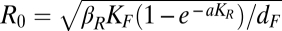, where β_R is the transmission rate from fleas to rodents, K_R is the rodents’ carrying capacity, K_F is the fleas’ carrying capacity per rodent, a is the flea-searching efficiency, and 1/d_F is the expected length of the infectious period; the term 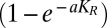is the probability of fleas searching successfully for a new rodent host.

On this basis, the first threshold quantity, R_eff, is then given by 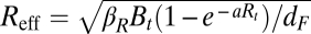. In other words, R_eff is defined as the product of the following three terms: (i) the density-adjusted transmissibility of the bacterium, (ii) the probability of the vector finding a new primary rodent host, and (iii) the expected length of the infectious period. The threshold quantity R_eff is found, therefore, to depend on R_t and B_t. In the statistical model, if the (lagged) rodent density is above some threshold in the spring (3.25 gerbils/hectare) and fall (4.94 gerbils/hectare), plague outbreaks may occur in the wildlife reservoir. Above that threshold, the infectious-flea force increases with the infectious-flea force of the previous year and the increase in the infectious-flea force since the previous season as well as the summer precipitation (Fig. 1). We note that the idea of this threshold quantity is based on the assumption that fleas and rodents mix homogeneously and that the main biological process is that of fleas searching for hosts. One can state that R_eff > 1 is a necessary condition for outbreaks. It has earlier been shown (15) that this condition is not sufficient for major outbreaks to occur in the Kazakhstan wildlife reservoir, because the spatial metapopulation of burrow systems causes percolation-like phenomena, violating the homogeneous mixing on which the above threshold concept is based. However, the condition is still necessary, because outbreaks start with local transmission being strong enough and locally homogeneous mixing can be a good approximation, even in case of a metapopulation. Furthermore, the threshold quantity describes threshold behavior in the classic sense in that a steady state of a dynamical system changes stability when the value of the quantity passes the threshold. We show next that the condition R_eff > 1 is also not sufficient for generating major outbreaks in the human population by spillover.

The second threshold for which we observed evidence statistically relates to the spread of plague into the human population. This threshold phenomenon cannot be explained by an R₀-like quantity as above. Among other factors, our analysis shows that the lagged flea density plays an important role in determining the dynamics of the system. We refer to a possible threshold quantity governing these dynamics as λ, which is described and reported here. The transmission process from wildlife reservoirs to humans is not fully understood; however, it is likely to be primarily a stochastic process and not the result of homogeneous mixing between humans and the wildlife reservoir. It is, therefore, not yet possible to propose a dynamic transmission model for the human exposure process from which to derive a quantity that possibly governs the stability of steady states in such a model. Theoretical work is certainly needed on the nature of this second threshold. It is our hope that our statistically based modeling study will stimulate such theoretical work.

We can, however, investigate what such a quantity could look like by a heuristic bottom-up approach to human exposure that can guide more fundamental future modeling. Instead of taking fleas or rodents as our starting point, we start from contacts by humans with the natural system. We concentrate on the flea route of transmission to humans. Let c be the stochastic number of lifetime contacts that a random susceptible human has to the rodent/flea natural system. Let c have a negative binomial distribution, with parameters 1 and 0.002, because most people have no contacts at all in present day and only a few people will have relatively many contacts (SI Text). Let, furthermore, m be the number of fleas that jump to a human given a contact and successfully transmit; m is assumed to have a Poisson distribution with a mean of the average number of fleas per rodent in the system, which depends on the flea density. Finally, let y be the prevalence of infected rodents in the system, where we assume that all fleas on an infected rodent are infective. Although a simplification, it is probably not far from true for septisemic gerbils when considering transmission by unblocked fleas (i.e., without latency period) (7). We define λ as the mean of the distribution governing the product cmy of these quantities. We obtain a value for λ by doing simulations using the different distributions based on the observed rodent prevalence and the observed flea to rodent ratios, all with a lag of 1 y. In Fig. 2C, we show a plot of λ based on a simulation with 10,000 replications as a function of the lag-1 flea density. The mean λ seems to be a suitable threshold quantity for spillover to humans. If its value is smaller than one, then we expect a minor sporadic number of human cases; if its value is larger than one, we expect major human outbreaks. There is a good correspondence with the statistically observed threshold phenomenon. This finding is to be expected, because λ depends on the lag-1 flea density. The epidemiological reasoning underlying λ, however, and the fact that its interpretation yields a natural threshold (both in contrast to the lag-1 flea density by itself) lead us to expect that a possible mechanistic threshold quantity, to be derived from a dynamic model describing the process of transmission to humans, will be strongly related to the quantity λ.

These results suggest that the spread of plague between rodents within the reservoir and from rodents to humans requires both high abundances of rodent hosts and a sufficient number of active fleas. Plague outbreaks in rodents occur [incurring the force of infection (17) to be strictly positive] only if the abundance of great gerbils (at the appropriate time lag) is above the critical threshold, in which case the force of infection varies with the change in the infectious-flea force of the previous season and the lag-1 infectious-flea force in addition to some climate variables, which are displayed in Fig. 1A.

The transmission rate to humans is a key determinant of the corresponding quantity λ, generating a threshold-type dynamic in humans, which is displayed in Fig. 2 A–C. There has to be a sufficient number of viable fleas (fleas ha⁻¹) for major human outbreaks to occur, which is shown in Fig. 2 B and C. In particular, high human transmission rates are predicted in the year after a high flea burden and a high infectious-flea force along with environmental conditions favorable for plague. Considering the full plague–wildlife–human system, R_eff > 1 is a necessary but not sufficient condition for plague outbreaks in the human population; for outbreaks to occur, it is also necessary that λ > 1. Hence, the rodent density and flea density (at appropriate time lags) are key threshold variables that determine when major human outbreaks may occur: the flea density is, in our analysis, found to be a major threshold variable in plague transmission to humans. The transmission of the disease to humans is, in fact, delayed by 1 y, which is indicated by the lag of the threshold variable (i.e., the lag-1 flea density) relative to its invasion of the reservoir.

Environmental factors affect the plague system at many levels (1, 5, 6), several of which are related to the effects of temperature and humidity on the reproduction and survival of hosts and vectors. Above the flea threshold, we find lag-1 spring temperature to be positively related to human plague cases, consistent with earlier findings that this relationship increases plague prevalence in gerbils (6). Below the flea threshold, warmer summers and wetter falls (at lag-1) decrease the probability of human infections. High summer temperatures are known to be detrimental to flea populations (6, 18). Precipitation in the fall might affect the quality of the burrows and the capacity for the rodents to keep warm in a wet and cold environment; under such conditions, the activity of the rodents may be suppressed (the rodents stay inside their burrows), and therefore, the chance of spreading the plague between burrow colonies is decreased.

The large-scale wildlife reservoir dynamics are dominated by several interlinked factors. The rodent population growth rate decays exponentially with the lag-1.5 flea density in the spring season and the lag-2 flea density in the fall season (being consistent with our earlier finding) (6); the upper regime of the change in the infectious-flea force model shows that an increase in the lag-1 infectious-flea force corresponds, in both seasons, to an increase in the current infectious-flea force when all other things are equal.

Our analysis suggests that summer precipitation plays a key role in the dynamics: it is positively linked with the fall flea burden, the change in the infectious-flea force in the upper regime of the fall season, and ultimately, the infectious-flea force in the upper regime of the fall (Fig. 1C). From Table 1, with other things being equal and when the lag-1 flea density is above the threshold, increasing the lag-1 spring temperature is associated with an increase in the human plague outbreaks (Fig. 2D). In fact, a 1 °C increase in lag-1 spring temperature during the study period increases the human outbreaks in the upper regime from an average of 2.82 to 4.59, a 63% increase. However, the climatic effects on the human plague outbreaks in the upper regime are amplified with the lag-1 infectious-flea force, which is positively affected by the summer rainfall. The model predicts that, in the upper regime, a 10% increase in infectious-flea force and a 1 °C increase in spring temperature (in the preceding year) would boost the human outbreaks from an average of 2.82 to 4.99, a 77% increase.

We assessed the empirical forecasting performance of the full ecoepidemiological model by fitting the model to the data from 1949 to 1990 and computing biannually the out of sample point forecasts in the rodent–flea–plague model (Fig. S6), conditional on which we compute the point forecasts and the 95% interval forecasts for the number of human plague cases from 1991 to 2003. The forecasts obtained (Fig. 2E) track the observed number of plague cases that are all within the 95% interval forecasts closely, except for the years 1998 and 1999; the reasons for the discrepancy are unclear.

By bringing together data on the dynamics of the full ecoepidemiological plague system, we have shown that the close link between the wildlife reservoir and the human population makes understanding the dynamics of the human component impossible in isolation from the dynamics of the plague within the reservoir. If we are to reduce the chances of a human plague outbreak, we will need to focus on the reservoir dynamics and the link between the reservoir and the human population. Hence, establishing close links between veterinary and human medicine, together with environmental scientists, is essential as is studying more closely the mechanisms involved in the human exposure process.

Methods

Statistical Modeling.

Seasonal wildlife reservoir model.

Both the original and the log-transformed rodent densities are highly skewed. Hence, we investigate the seasonal behavior of the rodent population growth rate that is denoted by G_t, where G_t = log(R_t/R_{t − 1}) and R_t is the rodent density averaged across all sites at time t. Simultaneously, we explore the seasonal dynamic behavior of the fleas depicted by the flea burden and the number of free infectious fleas that are searching for a host. The flea burden, denoted by B_t, is measured by B_t = log(F_t/R_t), where F_t is the flea density averaged across all sites at time t. The number of seasonal free infectious fleas that are searching for a host is denoted by I_t and computed as the product of the flea density and the prevalence of plague in rodents averaged across sites. We refer to I_t as the infectious-flea force.

We consider the following statistical model that investigates the seasonal dynamic behavior of both the rodents and fleas. Let the sub- and superscripts s and f refer to the spring and fall seasons, respectively. Using a similar approach as the approach used by Stenseth et al. (6) and Samia et al. (19) (Fig. S1A), we investigate a model in which the infectious-flea force I_t is a degenerate random variable such that I_t = 0 if t is spring and the lag-l^s rodent density, namely R_{t − l}^s, is below the spring threshold z^s and I_t = 0 if t is fall and the lag-l^f rodent density, namely R_{t − l}^f, is below the fall threshold z^f. The delay parameters l^s and l^f and the threshold parameters z^s and z^f are specified separately for the two seasons, and then, using a similar approach as the works by Stenseth et al. (6) and Samia et al. (19), we establish that a model incorporating these thresholds is better than alternatives lacking a threshold or using the same threshold in spring and fall (results of the bootstrap tests are given in SI Text). Otherwise, in the upper regime (i.e., when the threshold variable R_{t − l}^j is above the threshold parameter l^j, where j = s for spring and j = f for fall), the infectious-flea force I_t is highly skewed, and hence, we instead model a measure of the change in free infected fleas given by _t = log(1 + I_t) − log(1 + I_{t − 1}), referred to as the change in infectious-flea force, where one is added inside the logarithm because the infectious-flea force I_t can be zero. Then, in the upper regime for both seasons, the conditional distribution of (G_t,s, G_t,f, B_t,s, B_t,f, _t,s, _t,f) in year t is multivariate normal with mean 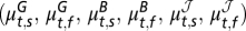and variance–covariance matrix Σ. The sub- and superscripts G, B, and refer to the rodent growth rate, flea burden, and change in infectious-flea force models, respectively. The structure of the variance–covariance matrix Σ is used to model possible heteroscedasticity and dependence among the observations (i.e., the diagonal entries of Σ are σ_i², i = 1, …, 6, where the σ_i², i = 1, …, 6 are not necessarily equal and the off-diagonal entries of Σ are not necessarily zero) (SI Text). Note that if, for example, the infectious-flea force in the spring season is in the lower regime, the variance–covariance matrix of the conditional distribution would have dimension reduced by one (i.e., the number of seasons in the lower regime). The serial correlation structures in the variance–covariance matrix that we considered are the general, compound symmetry, and autoregressive moving average structures (20).

Fig. S1B shows that the rodent growth rate decays exponentially with the flea density at different lags. Hence, we model the seasonal conditional means of the rodent growth rate nonlinearly as follows: where F_{t − d^s} and F_{t − d^f} are the lagged flea density for the spring and fall seasons, respectively. The vector of covariates and are season-specific. The delay parameters d^s and d^f are assumed to be season-specific and unknown; thus, they need to be estimated. The prime superscript signifies the transpose of the given vector.

Furthermore, we define the conditional means of the flea burden and the change in infectious-flea force models to be 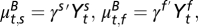The covariates , j = s, f in the flea burden model and in the change in infectious-flea force model are assumed to be season-specific.

Figs. 1A and 2A summarize the results of our analysis for year t ranging from 1949 to 1990. Using a similar approach as in the works of Stenseth et al. (6) and Samia et al. (19), we estimate the delay parameters l^s and l^f to be 1.5 and 2 y, respectively, and the threshold parameters z^s and z^f to be 3.25 and 4.94, respectively (the two numbers being significantly different) (SI Text). Fig. 1A summarizes the results of our analysis, where is the summer rainfall at time t. The subscript t − 0.5 refers to the previous season [i.e., if the response is in the spring (fall) of year t, then t − 0.5 refers to the fall of last year (spring of current year)]. The subscripts t − 1, t − 1.5, and t − 2 are similarly defined. Table 1 summarizes the maximum likelihood estimates of the parameters in the model along with their asymptotic SEs and asymptotic 95% confidence intervals. Model diagnostics are discussed in SI Text and in Figs. S2–S4.

Human–plague model.

We model the number of human plague cases in Kazakhstan using the newly introduced and developed generalized threshold model (GTM) in the work by Samia and Chan (11). Let ℋ_t be the number of infectious human cases in year t. Then, conditional on the vector covariate process {X_t}, ℋ_t is assumed to be an independent Poisson random variable with a conditional mean given by (Eq. 1)

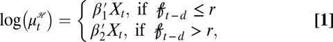where X_t is a p-dimensional vector of covariates that consists of the threshold variable _t and its lags as well as some other covariates and their lags. The vector covariate X_t may also contain lags of the response variable. The regression parameters are such that β₁ ≠ β₂, with β₁ and β₂ being p × 1 vectors. The parameter r is known as the threshold, and d is a nonnegative integer referred to as the delay or threshold lag. The analysis of the above model, referred to as a GTM, is conditional on the observed X values (11).

Our analysis is done by pooling information across all sites in the monitoring area and across all seasons (i.e., spring and fall seasons). Plague spread requires both a high abundance of hosts and a sufficient number of active fleas as vectors transmitting plague bacteria between hosts (6). Under this assumption, the threshold variable used in the model is the (lagged) flea density _{t − d} in year t − d, which is defined as the seasonal flea density averaged across all sites and then minimized across seasons (Table S2). The threshold variable considered in the GTM model is a measure of free fleas that are searching for a host. Let _t be a measure of the potential (annual) infectious-flea force to humans in year t, computed as the product of flea density and prevalence of plague in rodents, averaged across all sites and then maximized across seasons. Note that quantifies the number of infected fleas that could feed on and infect a human host (16, 21). Let be a measure of the flea burden in year t, computed as the ratio of the flea density divided by the rodent density, averaged across all sites and then maximized across seasons. Let be the density of the great gerbils in year t averaged across all sites and then maximized across seasons. Then, conditional on the vector covariate process {X_t}, the number of infectious human cases ℋ_t is assumed to be an independent Poisson random variable with a conditional mean given by Fig. 2A on the log scale, where is the spring temperature, is the summer temperature, and is the fall rainfall.

Fig. 2A summarizes the results of this analysis. The parameters, including the threshold parameter, were estimated by a likelihood-based approach. Table 1 summarizes the maximum likelihood estimates of the GTM defined in Fig. 2A. Note that the delay parameter d is estimated to be 1 y and that the threshold parameter r is estimated to be 148.71 using a grid search between the 10th and 90th percentiles of _t−1. Fig. 2B plots the number of infectious human plague cases vs. the threshold variable, namely the lag-1 flea density. The vertical line shows the location of the threshold estimate. Model diagnostics are discussed in SI Text and Fig. S5.

References

- 1.Stenseth NC, et al. Plague: Past, present, and future. PLoS Med. 2008 doi: 10.1371/journal.pmed.0050003. 10.1371/journal.pmed.0050003. [DOI] [PMC free article] [PubMed] [Google Scholar]
- 2.Pollitzer R. Plague. Geneva: World Health Organization; 1954. [Google Scholar]
- 3.Gage KL, Kosoy MY. Natural history of plague: Perspectives from more than a century of research. Annu Rev Entomol. 2005;50:505–528. doi: 10.1146/annurev.ento.50.071803.130337. [DOI] [PubMed] [Google Scholar]
- 4.Pollitzer R. Plague and Plague Control in the Soviet Union. Bronx, NY: Fordham University; 1966. [Google Scholar]
- 5.Kausrud KL, et al. Climatically-driven synchrony of gerbil populations allows large-scale plague outbreaks. Proc R Soc Lond B Biol Sci. 2007;274:1963–1969. doi: 10.1098/rspb.2007.0568. [DOI] [PMC free article] [PubMed] [Google Scholar]
- 6.Stenseth NC, et al. Plague dynamics are driven by climate variation. Proc Natl Acad Sci USA. 2006;103:13110–13115. doi: 10.1073/pnas.0602447103. [DOI] [PMC free article] [PubMed] [Google Scholar]
- 7.Eisen RJ, et al. Early-phase transmission of Yersinia pestis by unblocked fleas as a mechanism explaining rapidly spreading plague epizootics. Proc Natl Acad Sci USA. 2006;103:15380–15385. doi: 10.1073/pnas.0606831103. [DOI] [PMC free article] [PubMed] [Google Scholar]
- 8.Park S, et al. Statistical analysis of the dynamics of antibody loss to a disease-causing agent: Plague in natural populations of great gerbils as an example. J R Soc Interface. 2007;4:57–64. doi: 10.1098/rsif.2006.0160. [DOI] [PMC free article] [PubMed] [Google Scholar]
- 9.Begon M. Epizootiologic parameters for plague in Kazakhstan. Emerg Infect Dis. 2006;12:268–273. doi: 10.3201/eid1202.050651. [DOI] [PMC free article] [PubMed] [Google Scholar]
- 10.Frigessi A, et al. Bayesian population dynamics of interacting species: Great gerbils and fleas in Kazakhstan. Biometrics. 2005;61:230–238. doi: 10.1111/j.0006-341X.2005.030536.x. [DOI] [PubMed] [Google Scholar]
- 11.Samia NI, Chan KS. Maximum likelihood estimation of a generalized threshold stochastic regression model. Biometrika. 2011;98:433–448. [Google Scholar]
- 12.Salkeld DJ, Salathé M, Stapp P, Jones JH. Plague outbreaks in prairie dog populations explained by percolation thresholds of alternate host abundance. Proc Natl Acad Sci USA. 2010;107:14247–14250. doi: 10.1073/pnas.1002826107. [DOI] [PMC free article] [PubMed] [Google Scholar]
- 13.Sapozhnikov V, Serzhan OS, Bezverkhni AV, Kovaleva GG, Kopbaev ES. Plague in the Balkhash—Alakol Depression. Almaty, Kazakhstan: Rakhat; 2001. [Google Scholar]
- 14.Davis S, et al. Predictive thresholds for plague in Kazakhstan. Science. 2004;304:736–738. doi: 10.1126/science.1095854. [DOI] [PubMed] [Google Scholar]
- 15.Davis S, Trapman P, Leirs H, Begon M, Heesterbeek JAP. The abundance threshold for plague as a critical percolation phenomenon. Nature. 2008;454:634–637. doi: 10.1038/nature07053. [DOI] [PubMed] [Google Scholar]
- 16.Keeling MJ, Gilligan CA. Bubonic plague: A metapopulation model of a zoonosis. Proc Biol Sci. 2000;267:2219–2230. doi: 10.1098/rspb.2000.1272. [DOI] [PMC free article] [PubMed] [Google Scholar]
- 17.Anderson RM, May RM. Infectious Diseases of Humans: Dynamics and Control. Oxford: Oxford University Press; 1991. p. viii. [Google Scholar]
- 18.Krasnov BR, Khokhlova IS, Fielden LJ, Burdelova NV. Effect of air temperature and humidity on the survival of pre-imaginal stages of two flea species (Siphonaptera: Pulicidae) J Med Entomol. 2001;38:629–637. doi: 10.1603/0022-2585-38.5.629. [DOI] [PubMed] [Google Scholar]
- 19.Samia NI, Chan KS, Stenseth NC. A generalized threshold mixed model for analyzing nonnormal nonlinear time series, with application to plague in Kazakhstan. Biometrika. 2007;94:101–118. [Google Scholar]
- 20.Pinheiro JC, Bates DM. Mixed-Effects Models in S and S-PLUS. New York: Springer; 2000. p. xvi. [Google Scholar]
- 21.Keeling MJ, Gilligan CA. Metapopulation dynamics of bubonic plague. Nature. 2000;407:903–906. doi: 10.1038/35038073. [DOI] [PubMed] [Google Scholar]
Associated Data
This section collects any data citations, data availability statements, or supplementary materials included in this article.