Modelling the relationship between body fat and the BMI

Abstract

Objective

Given the increasing concerns about the levels of obesity being reached throughout the world, this paper analyses the relationship between the most common index of obesity, the BMI, and levels of body fat.

Research methods and procedures

The statistical relationship, in terms of functional form, between body fat and BMI is analysed using a large data set which can be categorized by race, sex and age.

Results

Irrespective of race, body fat and BMI are linearly related for males, with age entering logarithmically and with a positive effect on body fat. Caucasian males have higher body fat irrespective of age, but African American males’ body fat increases with age faster than that of Asians and Hispanics. Age is not a significant predictor of body fat for females, where the relationship between body fat and BMI is nonlinear except for Asians. Caucasian females have higher predicted body fat than other races, except at low BMIs, where Asian females are predicted to have the highest body fat.

Discussion

Using BMIs to make predictions about body fat should be done with caution, as such predictions will depend upon race, sex and age and can be relatively imprecise. The results are of practical importance for informing the current debate on whether standard BMI cut-off values for overweight and obesity should apply to all sex and racial groups given that these BMI values are shown to correspond to different levels of adiposity in different groups.

Introduction

In recent years both the medical profession and the media have become increasingly concerned about the levels of obesity being reached throughout the world. While body fat is arguably a direct measure of adiposity, its accurate measurement has traditionally required special equipment that has been costly to purchase and operate. Although direct measurement of body composition is becoming increasingly viable, attention has often been focused on the easier-to-measure body mass index (BMI), defined as the ratio of weight (in kilograms) to the square of height (in metres): see for example[1] for a survey of the historical development of the BMI. There are several assumptions inherent in the BMI-adiposity relationship. One such assumption is that BMI represents adiposity, independent of age, sex, and ethnicity/race: ie, the use of BMI assumes that, after adjusting a subject’s body weight for stature, all subjects have the same relative fatness regardless of their age, sex, or ethnicity. There have been several publications that have attempted to address these issues in children [2, 3] and adults [4, 5]. An overall conclusion is that there are many factors that influence the BMI-adiposity relationship and, where possible, a more direct assessment of fatness is recommended.

An interesting and related statistical problem is to assess the relationship between body fat and the BMI, which can include gauging the strength of the relationship, testing hypotheses concerning, for example, the functional form of the relationship, and using the fitted model for prediction. It is this aspect of the body fat-BMI relationship that we concentrate on in this paper.

Subjects and methods

This paper utilizes a relatively large data set containing body fat and BMI measurements to illustrate these facets of the analysis. The data set consists of body fat, height and weight of 1446 individuals, categorized by race and sex as in Table 1. The height and weight of the ith individual was combined as ${\mathit{\text{BMI}}}_i={\mathit{\text{weight}}}_i/{\mathit{\text{height}}}_i^2$. Results for the ‘Other’ category are not reported as the small number of observations either precluded estimation or led to very imprecise parameter estimates. These individuals had participated in body composition investigations [4, 6, 7] in the Body Composition Unit, St. Luke’s-Roosevelt Hospital and had body composition measured on a single dual-energy x-ray absorptiometry (DXA) scanner. The subjects were recruited from 1993 to 2001 through advertisements in local newspapers, on radio stations, and flyers posted in the local community.

Table 1.

Race and sex categorization of data. Numbers in parentheses denote outliers (see text).

Race	Male	Female	Total
African American	86 (3)	266 (0)	352 (0)
Asian	41 (0)	64 (0)	105 (0)
Caucasian	166 (3)	455 (0)	621 (3)
Hispanic	140 (2)	189 (3)	329 (5)
Other	23 (0)	16 (0)	39 (0)
All	456 (8)	990 (3)	1446 (11)

Inclusion in the study required that subjects be ambulatory with no orthopaedic problems or medical conditions known to affect body composition. Race was determined by self-report. All studies were approved by the Institutional Review Board of St. Luke’s-Roosevelt Hospital and all subjects gave written consent to participate. Body weight was measured to the nearest 0.2 kg and height to the nearest 0.5 cm using a stadiometer. Total body fat was measured in all subjects with a whole-body DXA scanner [8].

The statistical model

There are a variety of approaches to modelling the links between body fat and the BMI: for example, the individual impact on body fat of height and weight changes may be investigated or the physical restrictions on the range of body fat values may be imposed in some other way. The approach followed here emphasizes the idea that the choice of functional form for the relationship between body fat (y) and the BMI reflects the desire to model, as appropriately as possible, the conditional mean function E(y|BMI). The popularly employed inverse, semi-logarithmic and double logarithmic functional forms are all nested within the specification

$$y_i^{(\mathrm{\lambda })}={\beta }_0+{\beta }_{1}BM{I}_i^{(ø)}+u_{i}i=1,\dots ,n$$ (1)

where i denotes the ith individual from a sample of size n and, for y_i >0 and BMI_i >0 (restrictions which are, of course, always satisfied),

$$y_i^{(\mathrm{\lambda })}=\{\begin{array}{cc}(y_i^{(\mathrm{\lambda })}-1)/\mathrm{\lambda }& \mathrm{\lambda }\ne 0\\ \text{log}{y}_i\hfill & \mathrm{\lambda }=0\end{array}BM{I}_i^{(ø)}=\{\begin{array}{cc}(BM{I}_i^{(ø)}-1)/ø& ø\ne 0\\ \text{log}BM{I}_i\hfill & ø=0\end{array}$$

are Box and Cox transformations of the variables [9]. The stochastic nature of the relationship between y and BMI is made explicit by the inclusion of the error u_i, which is assumed to have zero mean and constant variance σ². The transformation parameters λ and ø, the regression parameters, β₀ and β₁, and the error variance σ² can be estimated by maximum likelihood using a nonlinear optimizing algorithm (see [9–11]: the Marquardt routine within the maximum likelihood procedure in Econometric Views 5 was used here). Assuming asymptotic normality of u_i, 70% and 95% confidence ellipsoids were constructed for the transformation parameters to aid interpretation, noting that setting λ = ø = 1 produces the linear model, λ = −ø = 1 produces the ‘inverse’ model, λ = ø = 0 produces the double logarithmic model and λ = 1, ø = 0 yields the semi-logarithmic model.

From (1), the conditional mean of y is given by

$$E\mathit{(}y|BMI\mathit{)}=\mathrm{E}\lfloor (\mathrm{\lambda }{({\beta }_0+{\beta }_{1}BM{I}_i^{(ø)}+u)}^{1/\mathrm{\lambda }}|BMI\_$$ (2)

Except for the linear model λ = ø = 1, the error u does not drop out of the expectation and must therefore be accounted for in making conditional predictions. The conditional mean was thus estimated using a ‘smearing’ technique, which uses estimated residuals to approximate the distribution of u required for the calculation of (2) [12, 13].

It is well known that the estimates of λ and ø can be badly affected by outliers and, as shown in Table 1, there are a small number of outlying observations in our data set. Eleven outliers are identified, all with unusually low body fat relative to BMI, and we concentrate on the models fitted to the data with these omitted (both visual and more formal identification schemes produced the same set of outliers). Including outliers tended to induce a greater degree of nonlinearity in the relationship than was found in the outlier-adjusted data. Even with such outliers omitted, the presence of a non-constant error variance may bias the estimates of the transformation parameters, so that we also investigated the use of a corrected likelihood function under the assumption that the error standard deviation is proportional to BMI, but this was found not to have any impact on the estimates [14]. Correlation between parameter estimates and the influence of data variability has been shown to have only marginal effects on model estimation [15].

Modelling the body fat – BMI relationship

Earlier research has shown that there are marked differences in the body fat-BMI relationship across sex and race [4, 5, 7]. We thus begin by reporting in some detail the fitting of model (1) to the data categorized by sex. For males, the ML estimates are (with standard errors shown in parentheses) λ̂ = 0.81(0.09) and ø̂ = 0.69 (0.34), leading to the regression model

$$\begin{array}{ccc}{y}_i^{(0.81)}\hfill & =-27.86+3.15BM{I}_i^{(0.69)}\hfill & {\widehat{\mathrm{\sigma }}}^2=7.29\hfill \\ \hfill & (12.42)(3.19)\hfill & \hfill \end{array}$$

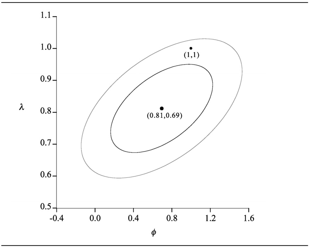
95% and 70% confidence ellipses for J = (λ,ø) are shown in Figure 1 and indicate that, of the conventional functional forms, only the linear (λ = ø = 1) is consistent with the data, with the functional forms conventionally used to model the body fat-BMI relationship all being rejected. There is thus little evidence of any nonlinearity in the body fat-BMI relationship for the outlier adjusted male data set and the relationship is therefore found to be linear, the estimated equation being

$$\begin{array}{cccc}{y}_i\hfill & =-34.08+1.98BM{I}_i\hfill & \widehat{\mathrm{\sigma }}=20.79\hfill & R^{\mathit{2}}=0.75\hfill \\ \hfill & (1.43)(0.05)\hfill & \hfill & \hfill \end{array}$$

Figure 1.

Male data (n = 448). Confidence ellipses for (λ, ø): outer ellipse, 95%; inner ellipse 70%.

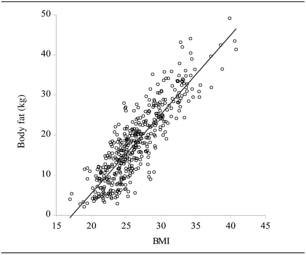
Figure 2 shows the scatter plot of body fat (y) against BMI with the linear fit superimposed. The conditional mean of y is thus linear, being E(y|BMI) = −34.08 + 1.98BMI, with the coefficient of 1.98 providing the marginal effect on y of a change in BMI, ie an increase in BMI of one unit is predicted to increase body fat by approximately 2 (±0.05) kg. Current US dietary guidelines define the range 18.5 < BMI < 25 to be ‘healthy’, 25 ≤ BMI < 30 to be ‘overweight’, and higher values of BMI to be ‘obese’ (see [1, table 2]). In the male sample here, 41.7% are healthy, 40.4% are overweight and 17.9% are obese (and 0.7% have BMIs below 18.5). Using standard results for the linear model, these cut-offs predict body fat weights of 2.6, 15.5 and 25.3 kg, respectively, with a standard error that is approximately 4.6 in each case. The fit also suggests the ‘rule of thumb’ that any value of BMI predicts a body fat of 2BMI – 34, although the width of the prediction intervals argues for regarding a particular BMI measure as providing only a rough indication of underlying body fat, particularly for low levels of BMI and body fat, for which the very few observations are only able to provide imprecise predictions.

Figure 2.

Males (n = 448). Scatter plot of body fat versus BMI with linear fit superimposed.

Table 2.

Functional forms for data categorised by sex and race.

Race	Male	Female
African American	λ̂= 0.72 (0.22), ø̂ = 0.44 (1.08) y = −34.5 + 1.96BMI	λ̂= 0.80 (0.10), ø̂ = 0.14 (0.22)
Asian	λ̂= 0.89 (0.71), ø̂ = 0.71 (2.08) y= −20.3 + 1.45BMI	λ̂= 0.18 (0.28), ø̂ = −0.17 (0.92) y= −22.6 + 1.77BMI
Caucasian	λ̂= 0.73 (0.15), ø̂ = −0.14 (0.75) y = −42.4 + 2.31BMI	λ̂= 0.85 (0.06), ø̂ = 0.29 (0.16)
Hispanic	λ̂= 1.06 (0.16), ø̂ = 1.31 (0.53) y = −30.7 + 1.83BMI	λ̂= 0.56 (0.12), ø̂ = −0.75 (0.39)

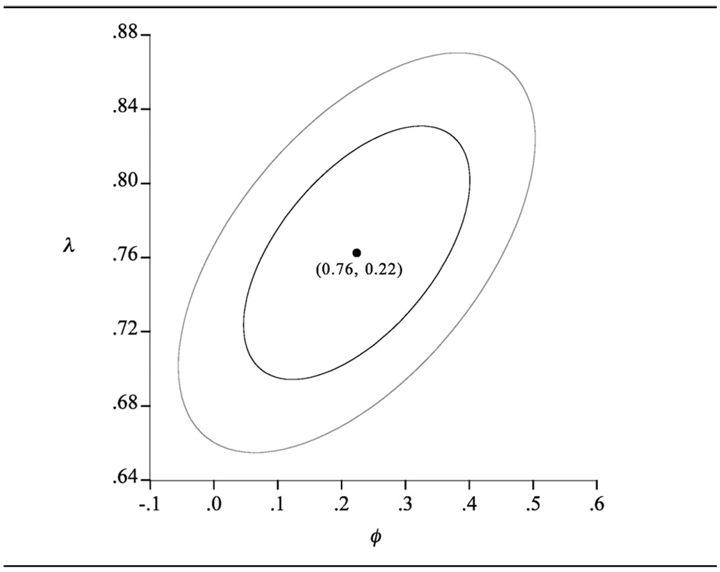
For females the ML estimates are λ̂= 0.76, ø̂ = 0.22. Here the linear model (λ = 1, ø = 1) is not contained within the 95% ellipse (see Figure 3) and neither are any other ‘simple’ functional forms. The ML model estimates are

$$\begin{array}{c}\begin{array}{cc}\widehat{\mathrm{\lambda }}=0.76(0.04)\hfill & \widehat{ø}\hfill \end{array}=0.22(0.11)\hfill \\ \begin{array}{ccc}{y}_i^{(0.76)}\hfill & =-43.49+11.87BM{I}_i^{(0.22)}\hfill & {\widehat{\sigma }}^2=3.60\hfill \\ \hfill & (7.98)(0.14)\hfill & \hfill \end{array}\end{array}$$

Figure 3.

Female data (n = 1435). Confidence ellipses for (λ, ø): outer ellipse, 95%; inner ellipse 70%.

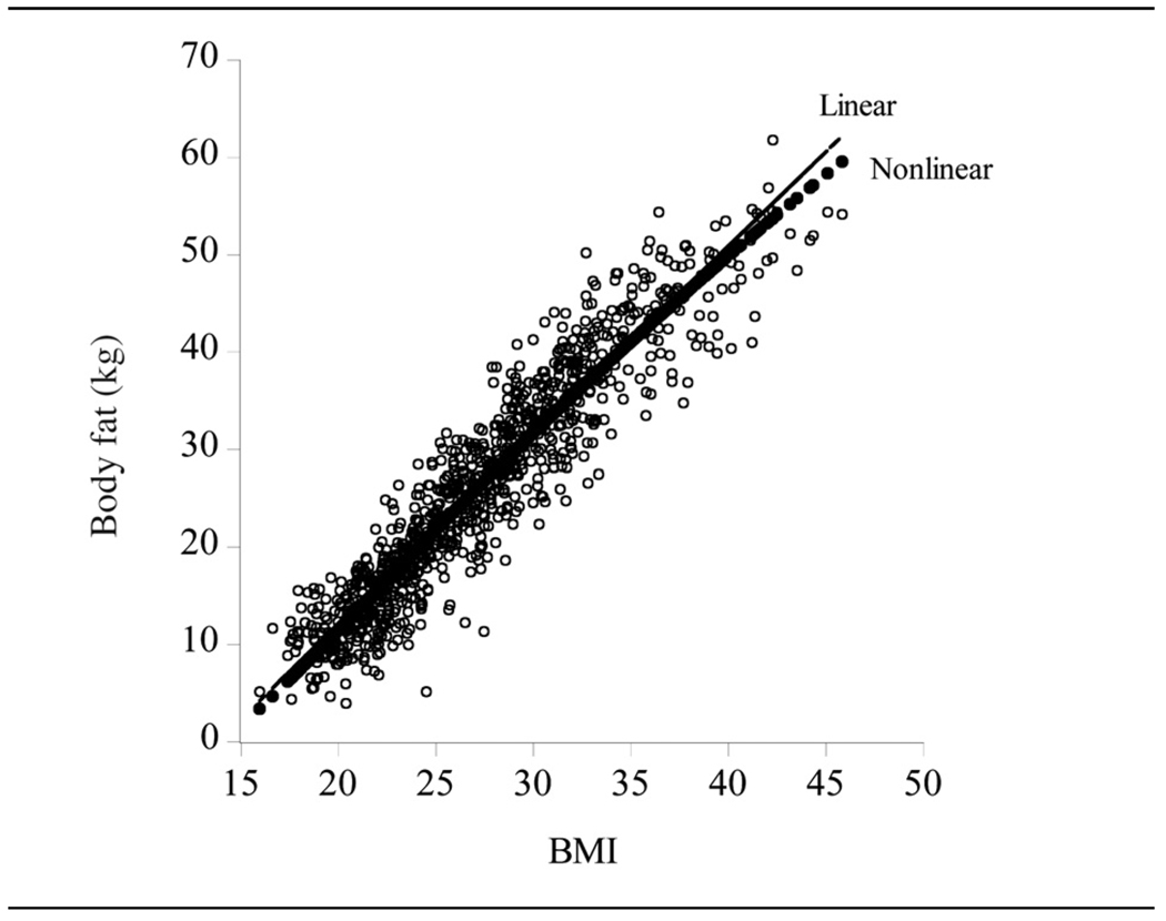
There is thus evidence of nonlinearity in the body fat – BMI relationship for the outlier adjusted female data set. Figure 4 shows the scatter plot of female body fat (y) against BMI with the nonlinear, $y_i^{(0.76)}=-43.49+11.87BM{I}_i^{(0.22)}$, and linear, y = −26.73 + 1.94BMI, fits superimposed. Although the statistical fit of the linear model is significantly inferior to that of the nonlinear models (the log-likelihoods of the two models are −1394.73 and −1378.84 respectively), the nonlinearity inherent in the relationship is rather modest, revealing itself primarily at the extremes of the sample, where the linear model over-predicts body fat.

Figure 4.

Females (n = 987). Scatter plot of body fat versus BMI with linear and nonlinear fits superimposed.

The conditional predictions of body fat at the cutoffs, using equation (2), are 8.6, 21.9 and 31.8 kg, with one standard error prediction intervals of (5.7,11.9), (18.1,26.0) and (27.6,36.2). The central predictions are just over 6 kg higher than for males and confirm previous findings that females have higher levels of body fat associated with a given BMI value [4].

The same procedure fitted to the complete data set produces ML estimates λ̂= 0.91(0.05) and ø̂ = 0.91 (0.13) and selects the linear model

$$\begin{array}{cccc}{y}_i\hfill & =-30.19+1.99BM{I}_i\hfill & {\widehat{\sigma }}^2=26.83\hfill & R^{\mathit{2}}=0.80\hfill \\ \hfill & (0.72)(0.03)\hfill & \hfill & \hfill \end{array}$$

This is found to over-predict male body fat by 4 kg and under-predict female body fat by 2 kg, as well as implicitly assuming a linear model for the female relationship. Categorizing by sex is thus seen to be essential for uncovering the appropriate body fat-BMI relationship.

Do these disparate findings for males and females carry over when the data set is categorized by race as well as sex? Table 2 schematically presents the results for this categorization of the data. In several cases the transformation parameters are quite imprecisely estimated because of the rather small sample sizes in some categories. Determining the appropriate functional form is therefore somewhat problematic, but linear functional forms are found to be acceptable for all male categories, although Caucasian males are just as well fitted by a semi-logarithmic function (λ = 1, ø = 0). Except for Asians, females continue to exhibit a non-linear relationship between body fat and BMI. When analysing the Asian data, for which the number of observations is relatively small anyway, further outliers became apparent. The results presented in Table 2 are with four outliers excluded for Asian females, all of which have unusually large values of both body fat and BMI, and whose inclusion induced a nonlinear fit having a perverse shape in which the second derivative of the function was positive. Excluding these outliers, while producing a linear fit, truncates an already small sample to one containing no individuals with BMIs in excess of 26.5. On the other hand, including the four outliers in the linear fit produces estimates that are almost identical to those reported in Table 2.

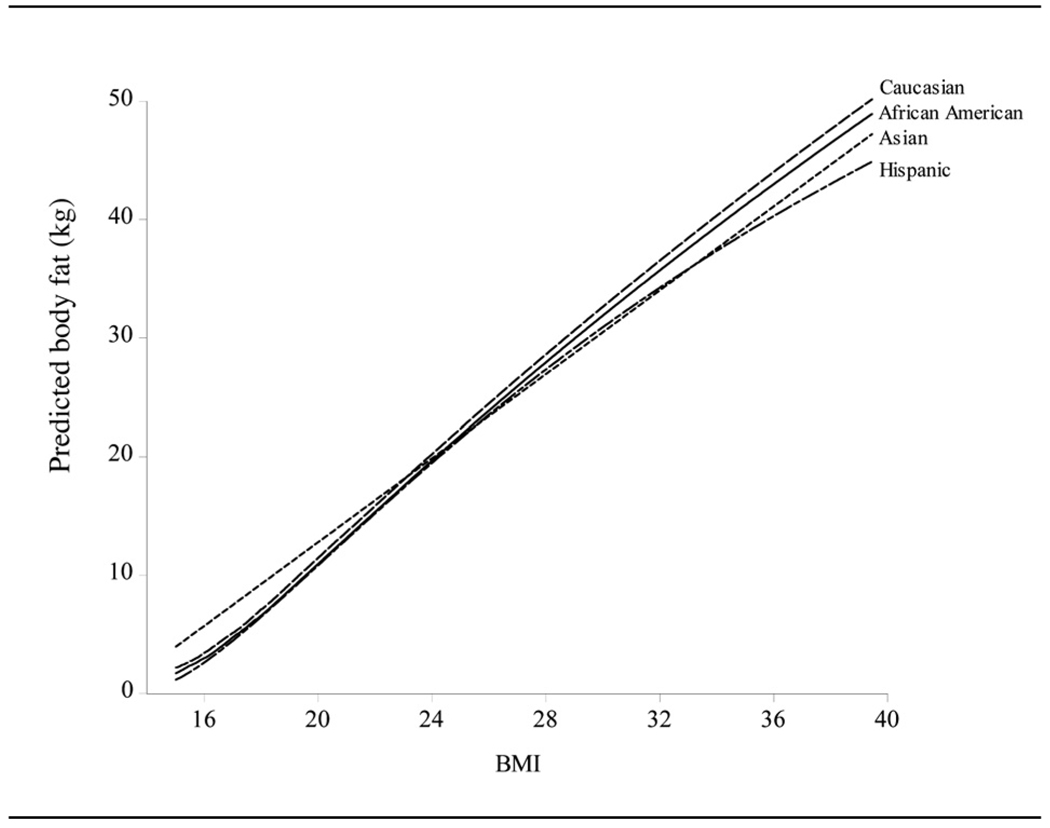
Figure 5 shows the estimated conditional mean functions for females categorized by race, and thus brings into focus the form and strength of the nonlinearity present in the body fat-BMI relationship. Although the functional forms are much closer to linearity than the forms generally assumed for the body fat-BMI relationship, modest nonlinearity still prevails. Apart from Asian females, for which the slope is constant at 1.77, the other three races all show a similar pattern of a brief steepening in slope up to a BMI of around 20, followed by a declining slope, which is more pronounced for Hispanics than for African Americans and Caucasians, whose body fat responses to changing BMI are very similar. The nonlinearity is thus found to be stronger at lower levels of the BMI, and for Hispanics in general.

Figure 5.

Estimated conditional mean functions for females categorized by race.

The body fat predictions at the standard BMI cutoffs, with approximate one standard error bounds, are reported for both males and females in Table 3. The steeper and flatter slopes, respectively, of the relationship for Caucasian and Asian males are readily apparent in the predictions, so that the Caucasian male predicted body fat response to an increase in BMI is much more pronounced than that for the Asian male, with African Americans and Hispanics having similar responses. This is also seen in females, with Caucasians having higher predicted body fat, except at low BMIs, where Asian females are predicted to have the highest body fat.

Table 3.

Predicted body fat (kg) from selected models.

Males
BMI	African American	Asian
18.5	y = 1.8 ± 3.6	y = 6.5 ± 2.9
25	y = 14.5 ± 3.6	y = 15.9 ± 2.9
30	y=24.3 ± 3.6	y =23.2 ± 2.9
BMI	Caucasian	Hispanic
18.5	y = 0.3 ± 4.8	y = 3.2 ± 4.2
25	y= 15.3 ± 4.8	y= 15.0 ± 4.2
30	y=26.9 ± 4.8	y =24.2 ± 4.2
Females
BMI	African American	Asian
18.5	y = 7.5 ± 4.1	y = 10.1 ± 2.9
25	y =21.8 ± 4.1	y =21.6 ± 2.9
30	y = 31.9 ± 4.1	y =30.5 ± 2.9
BMI	Caucasian	Hispanic
18.5	y = 8.0 ± 4.1	y = 7.4 ± 3.7
25	y =22.3 ± 4.1	y =21.5 ± 3.7
30	y =32.6 ± 4.1	y =30.9 ± 3.7

Including age as an additional regressor

The model (1) can be extended to include age as an additional Box-Cox transformed regressor:

$$\begin{array}{cc}{y}_i^{(\mathrm{\lambda })}={\beta }_0+{\beta }_{1}BM{I}_i^{(ø)}+{\beta }_{2}AG{E}_i^{(\mathrm{\theta })}+u_i& i=1,\dots ,n\end{array}$$

that can be estimated in a similar fashion to the bivariate model. Because the bivariate models have revealed marked sex-specific relationships, we present first the models fitted to the male and female data respectively. For males, the model is

$$\begin{array}{c}\widehat{\mathrm{\lambda }}=0.80(0.09)\widehat{ø}=0.72(0.31)\widehat{\theta }=0.45(0.85)\hfill \\ y=-45.81+1.95BMI+3.29\text{log}AGE\widehat{\mathrm{\sigma }}=4.363R^{\mathit{2}}=0.77\\ (2.26)(0.05)\hfill \end{array}$$

Including AGE has no impact on the estimates of λ and ø nor on the marginal effect of BMI (the correlation between AGE and BMI is only 0.05, so that these variables are almost orthogonal). The model (λ = 1, ø = 1, θ = 0) provides the best ‘simple’ functional form fit. Compared to the bivariate model y = −34.1 + 1.98BMI, this model allows predicted body fat, conditional on a BMI value, to alter with (the log of) AGE. For example, at AGE = 20, predicted body fat is −35.95 + 1.95BMI, while at AGE = 60, the prediction is given by −32.34 + 1.95BMI, some 3.5 kg higher. At the obesity cut-off of BMI = 30, these functions therefore predict body fat to be 22.6 kg and 26.2 kg, compared to the prediction of 25.3 kg which ignores the age effect.

For females, the model is

$$\begin{array}{c}\widehat{\mathrm{\lambda }}=0.76(0.05)\widehat{ø}=0.23(0.11)\widehat{\theta }=-1.76(19.43)\hfill \\ \begin{array}{cc}{y}^{(0.76)}\hfill & =-59.55+11.91BM{I}^{(0.23)}+27.70AG{E}^{(-1.76)}\hfill \\ \hfill & (55.01)(0.15)(97.23)\hfill \end{array}\hfill \\ {\mathrm{\sigma }}^{^}=1.89R^{\mathit{2}}=0.88\hfill \end{array}$$

Here the inclusion of AGE produces an extremely imprecise estimate of θ and, indeed, AGE^(θ̂) is found to be insignificant anyway, implying that AGE has no influence on the y – BMI relationship for females.

These findings also characterize the racial categorizations as well. For no female/race category is the influence of AGE significant, while for every male/race category, logAGE is found to be significant when added to the linear y – BMI model obtained initially. Table 4 reports these models along with the predicted body fat for each race conditional on AGE. Thus, a 30-year-old African-American male with BMI = 30 would be predicted to have body fat of 22.4±3.6 kg, while similar Asian, Caucasian and Hispanic males are predicted to have body fats of 22.5±2.9, 24.9±4.8 and 23.3±4.2 kg, respectively. At age 60, these predictions would be 25.4±3.5, 24.3±3.6, 28.2±4.8 and 24.8±4.2 kg. Thus Caucasian males have higher body fat irrespective of age, but African American males’ body fat increases with age faster than Asians and Hispanics.

Table 4.

Predicted male body fat (kg) conditional on AGE.

AGE	African American y = −52.2 + 2BMI + 4.3 log AGE	Asian y = −29.2 + 1.44BMI+ 2.5log AGE
20	y = −52.2 + 2BMI ± 3.7	y = −21.7 + 1.44BMI ± 2.9
30	y= −37.6 + 2BMI ± 3.6	y = −20.7 + 1.44BMI ± 2.9
40	y = −36.3 + 2BMI ± 3.6	y = −20.0 + 1.44BMI ± 2.9
50	y= −35.4 + 2BMI ± 3.5	y = −19.4 + 1.44BMI ± 2.9
60	y= −34.6 + 2BMI ± 3.5	y = −18.9 + 1.44BMI ± 2.9
70	y = −33.9 + 2BMI ± 3.5	y = −18.6 + 1.44BMI ± 2.9
AGE	Caucasian y = −57.4 + 2.2SM + 4.8log AGE	Hispanic y = −39.0 ± 1.83BM + 2.2log AGE
20	y = −43.0 + 2.2BMI ± 4.8	y = −32.5 + 1.83BMI ± 4.2
30	y = −41.1 + 2.2BMI ± 4.8	y = −31.6 + 1.83BMI ± 4.2
40	y = −39.7 + 2.2BMI ± 4.8	y = −31.0 + 1.83BMI ± 4.2
50	y = −38.6 + 2.2BMI ± 4.8	y = −30.5 + 1.83BMI ± 4.2
60	y = −37.8 + 2.2BMI ± 4.8	y = −30.1 + 1.83BMI ± 4.2
70	y = −37.0 + 2.2BMI ± 4.8	y = −29.8 + 1.83BMI ± 4.2

Conclusions

In this paper we have explored a large data set containing observations on body fat, BMI and age categorized by race and sex. Using sophisticated statistical methods, no evidence has been found to support the functional forms that have traditionally been proposed for modelling this relationship, for it appears that, irrespective of race, body fat and BMI are linearly related for males, with age entering logarithmically and with a positive effect on body fat. Where race makes an impact is in terms of the differential response of body fat to increases in BMI, with predicted body fat increasing more rapidly with higher BMI for Caucasian males and less rapidly for Asian males.

In contrast, age is not a significant predictor of body fat for females, but the relationship between body fat and BMI is nonlinear except for Asians, for which the sample is relatively small and contains very few individuals with large BMIs. This finding of nonlinearity is interesting in itself, as it may be of importance when studying and understanding the biology of energy stores. At the very least, it challenges researchers to explain the physiological processes that underlie the nonlinearity, which can amount to differences in up to 3 kg in predicted body fat compared to linear fits at the upper extremes of our data values and which is bordering on practical significance. Overall, Caucasian females have higher predicted body fat than other races, except at low BMIs, where Asian females are predicted to have the highest body fat.

In all categories, prediction standard errors are in the range of 3 to 5 kg, depending on sex and race (Asians have prediction standard errors of 2.9 kg, regardless of sex, while Caucasians have the largest standard errors: 4.8 kg for males and 4.1 kg for females). Thus using BMIs to make predictions about body fat should be done with caution, as they will depend upon race, sex and age and can have wide prediction intervals. Nevertheless, the findings reported here are of practical importance for informing the current debate on whether the standard BMI cut-off values for overweight and obesity (25 and 30 respectively) should apply to all sex and racial groups given that these BMI values are shown to correspond to different levels of adiposity in different groups.

References

- 1.Kuczmarski RJ, Flegal KM. Criteria for definition of overweight in transition: background and recommendations for the United States. Am J Clin Nutr. 2000;72:1074–1081. doi: 10.1093/ajcn/72.5.1074. [DOI] [PubMed] [Google Scholar]
- 2.Pietrobelli A, Faith M, Allison DB, et al. Body mass index as a measure of adiposity among children and adolescents. J Paed. 1998;132:204–210. doi: 10.1016/s0022-3476(98)70433-0. [DOI] [PubMed] [Google Scholar]
- 3.Cole TJ, Faith M, Pietrobelli A, et al. What is the best measure of adiposity change in growing children: BMI, BMI%, BMI z-score or BMI centile? Eur J Clin Nutr. 2005;59:419–425. doi: 10.1038/sj.ejcn.1602090. [DOI] [PubMed] [Google Scholar]
- 4.Gallagher D, Visser M, Sepulveda D, et al. Body mass index as an estimate of fatness across sex, age, and ethnic groups. Am J Epid. 1996;143:228–239. doi: 10.1093/oxfordjournals.aje.a008733. [DOI] [PubMed] [Google Scholar]
- 5.Gallagher D, Heymsfield SB, Heo M, et al. Healthy percent fat ranges: an approach for developing guidelines based upon body mass index. Am J Clin Nutr. 2000;72:694–701. doi: 10.1093/ajcn/72.3.694. [DOI] [PubMed] [Google Scholar]
- 6.Wang J, Thornton JC, Burastero S, et al. Comparisons for body mass index and body fat per cent among Puerto Ricans, blacks, white and Asians living in the New York City area. Obes Res. 1996;4:377–384. doi: 10.1002/j.1550-8528.1996.tb00245.x. [DOI] [PubMed] [Google Scholar]
- 7.Fernandez JR, Heo M, Heymsfield SB, et al. Is percentage body fat differentially related to body mass index in Hispanic Americans, African Americans, and European Americans? Am J Clin Nutr. 2003;77:71–75. doi: 10.1093/ajcn/77.1.71. [DOI] [PubMed] [Google Scholar]
- 8.Mazess RB, Peppler WW, Chesnut CH, et al. Total bone mineral and lean body mass by dual-photon absorptiometry. II. Comparison with total body calcium by neutron activation analysis. Calcif Tissue Int. 1981;33:361–363. doi: 10.1007/BF02409456. [DOI] [PubMed] [Google Scholar]
- 9.Box GEP, Cox DR. An analysis of transformations. J Roy Statl Soc, Ser B. 1964;26:211–252. [Google Scholar]
- 10.Spitzer JJ. A primer on Box-Cox estimation. Rev Econ Stats. 1982;64:307–313. [Google Scholar]
- 11.Mills TC. Predicting body fat using data on the BMI. J Stat Educ. 2005;13:1–12. [Google Scholar]
- 12.Abrevaya J. Computing marginal effects in the Box-Cox model. Econom Rev. 2002;21:383–393. [Google Scholar]
- 13.Duan N. Smearing estimate: A nonparametric retransformation method. J Am Stat Assoc. 1983;78:605–610. [Google Scholar]
- 14.Seaks TG, Layson SK. Box-Cox estimation with standard econometric problems. Rev Econ Stats. 1983;65:160–164. [Google Scholar]
- 15.Yang Z, Abeysinghe T. An explicit variance formula for the Box-Cox functional form estimator. Ec Letts. 2002;76:259–265. [Google Scholar]