Use of tumor dynamics to clarify the observed variability among biochemical recurrence nomograms for prostate cancer

Abstract

BACKGROUND

Nomograms for biochemical recurrence (BCR) of prostate cancer (PC) after radical prostatectomy can yield very different prognoses for individual patients. Since the nomograms are optimized on different cohorts, the variations may be due to differences in patient risk-factor distributions. In addition, the nomograms assign different relative scores to the same PC risk factors and rarely stratify for tumor growth rate.

METHODS

We compared BCR-free probabilities from the GPSM model with a cell kinetics (CK) model that uses the individual’s tumor state and growth rate. We first created a cohort of 143 patients that reproduced the GPSM patient distribution in Gleason score, Prostate specific antigen (PSA), Seminal vesicle involvement and Margin status since they form the GPSM score. We then performed 143 CK calculations to determine BCR-free probabilities for comparison with the GPSM results for all scores and with four other prominent nomograms for a high-risk patient.

RESULTS

The BCR-free probabilities from the CK model agree within 10% with those from the GPSM study for all scores once the CK model parameters are stratified in terms of the GPSM risk factors and the PSA doubling time (PSADT). However, the probabilities from widely used nomograms vary significantly.

CONCLUSIONS

The CK model reproduces the observed GPSM BCR-free probabilities with a broad stratification of model parameters for PC risk factors and can thus be used to describe PC progression for individual patients. The analysis suggests that nomograms should stratify for PSADT to be predictive.

1. BACKGROUND

A man diagnosed with prostate cancer (PC) can use a variety of nomograms to evaluate his risk of biochemical recurrence (BCR) after radical prostatectomy (RP) [1–5] and PC specific death [6–8]. Such models can inform therapeutic decisions because they tabulate outcome probabilities based on thousands of patients at leading institutions. The BCR models consider various risk factors such as Gleason score (GS), tumor stage (TNM), margin status, involvement of seminal vesicles and lymph nodes, and serum prostate specific antigen (PSA). For example, the GPSM scoring algorithm [1] at the Mayo Clinic formulates the risk of BCR using a sum of GS and indices for PSA, margin status, and the involvement of seminal vesicles or lymph nodes. Memorial Sloan-Kettering Cancer Center (MSKCC) [2] uses similar risk factors in a different point system that also includes the TNM and date of RP. The UCSF Cancer of the Prostate Assessment (CAPRA) score [3] uses the patient’s age and percent of positive biopsies (PPB) in addition to PSA, GS and TNM. The Han Table [4] from Johns Hopkins uses PSA, GS and a single risk category for any regional involvement. D’Amico et al [5] define low-, intermediate- and high-risk strata for BCR after RP and radiation therapy (RT) based on PSA, GS and TNM.

Lughezzani et al. [9] compared three BCR models [2, 3, 5] and found that their ability to predict BCR in an independent cohort was limited to concordance indices of 67–74% at 5 yrs. Thus, a nomogram may be able to predict outcomes for the cohort used to derive its scoring system but not necessarily for other cohorts with different risk-factor distributions. The variability among nomograms is not surprising since they weigh or rank the same risk factors differently. For example, the relative contribution of GS to an individual’s score can vary significantly among the models (see Sec. 4). In addition, most BCR models are incomplete since they stratify risk factors associated with the tumor state at diagnosis but not its growth rate. Thus, patients with slow- and fast-growing tumors but with identical GS, PSA, and TNM would obtain identical pre-operative predictions from a nomogram even though they would expect to progress quite differently. Indeed, tumor dynamics is important since the time to BCR [10] and PC specific death [6–8] were both found to increase with PSA doubling time (PSADT). A related issue is that nomograms use different BCR endpoints, usually in terms of detectable PSA, and a twofold increase in PSA endpoint translates to a delay of one PSADT in the time to BCR for the same patient. Perhaps a deeper question arises as to how a patient with one set of risk factors utilizes outcome probabilities derived from different patient distributions, especially when the models disagree.

A tool aimed at an individualized prognosis and based on tumor dynamics was developed recently using a cell kinetics (CK) model [11]. The CK model uses coupled time-dependent equations for local, regional and systemic cell populations in order to describe PC progression from a local hormone-sensitive (HS) tumor to a systemic hormone-resistant (HR) disease. The model is initialized by the individual’s tumor state at diagnosis as characterized by GS, PSA, TV, TNM and regional involvement. The time variable is scaled to his measured PSADT since it characterizes the individual’s tumor growth rate. Such a description is possible for PC because serial PSA measurements can monitor progression. It is also useful for therapeutic management because PC is typically a slow growing disease. However, since the propensity for PC cells to produce PSA varies widely among men [12], an individual’s cell specific PSA (cell analog to PSA density) should be calibrated using his measured tumor volume (TV). Then, calibrated serial PSA measurements can be combined with CK calculations to update the individual’s PC progression quantitatively. Indeed, the CK model parameters were chosen [11] to reproduce PC survival studies [4–6] that stratified for PSADT. Since BCR precedes PC specific death, it may be possible to describe both using the same CK model parameters.

Here, we compare the CK model with the GPSM model by performing CK calculations on 143 individuals who collectively have the same PC risk-factor (GS, PSA, TV, regional invasion) distributions as the GPSM cohort [1]. This similarity is required because the CK model describes individuals in a deterministic manner whereas the GPSM model yields outcome probabilities based on its patient population. With similar patients, we can use the 143 calculated recurrence times from the CK model to generate BCR-free probabilities P_BCRF(GPSM, t) as a function of GPSM score and time t after RP. Since time is scaled to PSADT in the CK model, we use the median PSADT ~ 1.26 yr of the GPSM cohort to transform the results to calendar time. We obtain excellent agreement in P_BCRF with Thompson et al [1] using model parameters [11] that also describe clinical PC survival studies [6–8]. We also compare our results with the MKSCC, Han, D’Amico and CAPRA models for a high-risk patient, and find significant differences among them that could be related to missing risk factors such as PSADT. The clinical implication of our study is that BCR nomograms should stratify for tumor growth rate (e.g. PSADT) in addition to risk factors associated with the tumor state at diagnosis (e.g. GS).

2. MATERIALS AND METHODS

2.1 GPSM scoring algorithm

At the Mayo clinic, the risk of BCR is found to increase with the GPSM score [1], which consists of GS plus indices for the range of PSA (P), the involvement of seminal vesicles or lymph nodes (S), and the margin status (M), namely,

$$\text{GPSM}=\text{GS}+\text{P}+\text{S}+\text{M}$$ (1)

The indices P, S and M vary as described in Table 1. For example, a patient with GS = 9, PSA = 8 μg/L (P = 1), seminal vesicle involvement (S = 2) and positive margins (M = 2) has GPSM = 14. Such a patient is high-risk and could be given adjuvant therapy immediately after RP to delay recurrence. The GPSM score for those given immediate adjuvant therapy is reduced by 4 for hormone therapy (HT) and by 2 for RT.

Table 1.

Basic GPSM scoring algorithm

Parameter	Value
GLEASON SCORE	GS
PSA (μg/L)
0 ⇒ 3.9	P = 0
4 ⇒ 10	P = 1
10.1 ⇒ 20	P = 2
> 20	P = 3
SEMINAL VESICLES or LYMPH NODES
Negative	S = 0
Positive	S = 2
MARGINS
Negative	M = 0
Positive	M = 2
GPSM	GS+P+S+M

Thompson et al [1] constructed BCR-free probabilities P_BCRF(GPSM, t) as a function of GPSM and time t based on 2,728 patients who underwent RP at the Mayo Clinic from 1997 to 2001. They defined recurrence at PSA ≥ 0.4 μg/L and, as expected, their Fig. 1 shows that P_BCRF decreases monotonically with GPSM and time. Patients with GPSM ≤ 7 have good outcomes with P_BCRF ≥ 0.9 at 7 years whereas those at high-risk with GPSM ≥ 13 exhibit a P_BCRF that decreases quickly with time and thus may consider immediate adjuvant therapy. The GPSM model is also used at the Mayo Clinic to predict PC progression and death [1].

Figure 1.

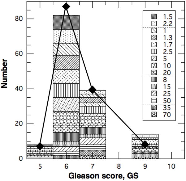
Histogram of patient population in Table 3 vs. Gleason score. Diamonds are for GPSM cohort from Table 2.

The characteristics of the men in the GPSM cohort [1] are reproduced for convenience in Table 2 and Figs. 1–4. Most patients (~66%) are low-risk with GS ≤ 6 and only 6% are high-risk with GS ≥ 8. We transformed the tumor dimensions into volumes by assuming the tumors are spherical, and obtained a median TV ~ 4–5 cc. Combining this with the median PSA ~ 6.4 μg/L gives a median PSA density of PSAD ~ 1 μg/L/cc, which is consistent with previous measurements [12] for PC. Of course, PSAD varies widely among men [12] but it can be calibrated for the individual as described in Sec. 2.3. The resultant distribution in GPSM is broad, as seen in Table 2, but most (88%) patients are within 3 points of the ‘median patient’ with a GPSM ~ 7 made up of GS ~ 6, pT2, TV ~ 4–5 cc, PSA ~ 6 μg/L, and negative margins.

Table 2.

Clinical and pathological features of 2,728 patients in GPSM cohort from Table 1 of Thompson et al [1] that are used to define patients for the CK model.

Parameter (units)	Value
Pathological Gleason score (%)
≤ 5	5.2
6	61.1
7	27.8
8 – 10	5.9
Maximum tumor dimension (%)		Inferred spherical tumor volume
0 – 1.4 cm	33.3	0 – 1.4 cc
1.5 – 2.4 cm	30.4	1.8 – 7.2 cc
2.5 – 2.9 cm	11.4	8.2 – 12.7 cc
≥ 3 cm	24.9	≥ 14.1 cc
Pathological tumor stage (%)
T2	82.4
T3a	9.1
T3b/4	6.5
Tx N+	2.0
GPSM score (%)
< 6	1.5
6	13.9
7	31.1
8	17.6
9	13.7
10	10.0
11	5.0
12	3.2
≥ 13	4.0
Positive margins (%)	30
PSA (μg/L)	0.2 – 144
Median	6.4
Median PSADT (yr)	1.26

Figure 4.

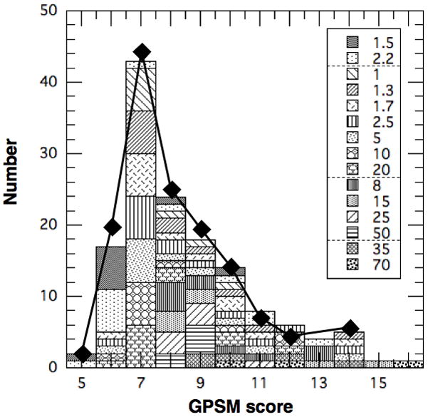
Histogram of patient population in Table 3 vs. GPSM score. Diamonds are for GPSM cohort from Table 2.

2.2 Cell Kinetics (CK) Model

The CK model was developed to describe an individual’s PC progression from diagnosis to death using time-dependent rate equations that are validated by clinical data. It is based on the observations that PC begins as a hormone sensitive (HS) localized tumor and gradually becomes hormone resistant (HR) as it spreads throughout the body. Also, PC is assumed to be curable if caught early and fatal when the total tumor burden exceeds some level. Such a progression can be described by postulating that PC has 3 dynamic cell populations: N_L for local HS cells, N_HS for regional HS cells and N_HR for systemic HR cells. The model is initiated by stipulating the size of the primary tumor N_L(0) at some reference time t = 0, which is estimated from the individual’s TV at biopsy or RP. Without therapy, it is assumed to grow as

$$N_L(t)=N_L(0)e^{0.693t/\mathit{PSADT}}=N_L(0)2^{t/\mathit{PSADT}}$$ (2)

to some maximum size N_Lmax since its ability to nourish itself diminishes with the surface to volume ratio. Metastasis is taken to occur when N_L reaches a critical size N_crit (≪ N_Lmax) because PC is likely cured [13] if treated early (i. e. N_L < N_crit). Indeed, Dattoli et al. [14] studied the interaction of a PC tumor with its host prostate and estimated a critical cell count for metastasis to be roughly 10⁹ – 10¹⁰ cells. When N_L exceeds N_crit, the systemic cells grow explosively from N_HS = N_HR = 0 as new tumor sites develop. Once established, systemic cells reproduce exponentially on their own and cause PC specific death when N_HS+N_HR ≥ N_PCD. In this model, the N_L and N_HS cells can be treated by HT and RT and N_HR by chemotherapy. The critical cell populations (N_crit, N_Lmax, N_PCD) and metastasis rate coefficient (α) were estimated [11] from clinical survival studies [6–8] within their limited stratifications.

The behavior outlined above can be quantified to any required mathematical complexity, but the existing clinical data can be described by a simplified set of coupled first-order differential equations [11], namely,

$$\frac{{dN}_L}{d\tau }=0.693N_L-\mathit{PSADT}\ast F_L(t)$$ (3a)

for a primary tumor N_L ≤ N_Lmax and

$$\frac{{dN}_{HS}}{d\tau }=0.693N_{HS}+\alpha N_L\mathrm{\Theta }(N_L-N_{\mathit{crit}})-\mathit{PSADT}\ast F_{HS}(t)$$ (3b)

$$\frac{{dN}_{HR}}{d\tau }=0693N_{HR}+\alpha N_{HS}-\mathit{PSADT}\ast F_{HR}(t)$$ (3c)

for the systemic populations. The factor 0.693 = ln(2) arises because time is scaled as

$$\tau \equiv \text{t}/\text{PSADT}$$ (4)

to conform to the clinical stratifications by PSADT. The Heavyside step-function Θ(N_L - N_crit) is used to describe a sudden onset of metastasis since Θ increases discontinuously from 0 to 1 when N_L exceeds N_crit. The initial metastasis is described as a mutation of N_L cells at a rate of α/PSADT. The metastasis rate coefficient α is small and depends on clinical risk factors such as GS. (Some terms have been omitted in Eq. 3 with little error because α ≪ 1.) The forcing functions F_L, F_HS and F_HR are used to represent therapies mathematically, as discussed by Dimonte [11].

The CK model is formulated in terms of PC cells because they are the fundamental constituents of tumors, but tumor sizes are characterized clinically by TV, TNM and PSA. To bridge the clinical and cellular views, we assume that PC cells contribute to PSA as

$$\text{PSA}={\text{PSA}}_{\text{O}}+{\text{K}}^{\ast }({\text{N}}_{\text{L}}+{\text{N}}_{\text{HS}}+{\text{N}}_{\text{HR}})$$ (5)

where PSA_o is the contribution from normal prostate cells and K is the cell specific PSA for PC in units of μg/L per cell. PSA_o can grow linearly in time as the prostate enlarges with age, but the PC component typically grows exponentially. We estimate

$$K=\frac{\mathit{PSA}}{\mathit{volume}}\frac{\mathit{volume}}{\mathit{cell}}\sim \mathit{PSAD}{D}^3\sim {10}^{-9}\frac{ng}{mL\ast \mathit{cell}}$$ (6)

by assuming a PC cell footprint D ~ 10 μm and an effective volume D³ ~ 10⁻⁹ cc. Since PSAD varies significantly among men [8], we estimate K for the GPSM cohort (Eq. 7) to relate PSA failure at 0.4 μg/L to a cell population.

The CK model is intended to describe an individual’s PC progression using his measured risk factors to set model parameters, which are inferred from clinical studies. However, most studies report population-based probabilities whereas the CK model describes an individual. To bridge these complementary views, Dimonte [11] distilled median PC survival times from clinical survival probabilities [6–8] for comparison with CK calculations. By stratifying the metastasis rate coefficient α for GS (i.e. α(GS)), the CK model [11] obtained median PC survival times in the range of 10–40*PSADT that agree with clinical observations [6–8]. Here, we use an alternate validation strategy that constructs BCR survival probabilities from many sample CK calculations for a hypothetical cohort with similar risk factors to those of a clinical study of interest. The GPSM cohort is chosen here for analysis because it has estimates for TV and PSADT, as required by the CK model, in addition to GS and other risk factors. The CK model uses the TV to initiate a calculation with N_L(0), and the median PSADT (1.26 yr) to transform the CK model’s scaled recurrence time τ_rec into calendar years after RP. We then vary α as a function of GS and regional invasion (S+M) in order to reproduce the P_BCRF(GPSM, t) observed in the GPSM study [1]. This comparison yields a metastasis rate coefficient α(GS, S+M) that is consistent with the α(GS) estimated previously for survival, but with the additional functional dependence on S+M given by the GPSM stratification for regional invasion.

2.3 Patient Distributions

To compare BCR probabilities constructed from individual CK calculations with those from the GPSM study, it is important to adopt a CK sample population that matches the GPSM risk factor distributions. The key characteristics of the GPSM cohort are summarized in Table 2 by strata pertaining to the scoring algorithm and factors used by the CK model. These characteristics are first reproduced in a cohort of 143 individuals and then each patient is modeled with a CK calculation from metastasis to PC specific death. In addition to GPSM scoring factors (GS, P, S and M), each CK calculation requires an estimate of the tumor volume and growth rate. The TVs are estimated from the dimensions in Table 2 and are broadly associated with PSA [12]. The PC growth rate is characterized by the median PSADT ~ 1.26 yr for the GPSM cohort. In this section, the CK men are described individually in Table 3 and compared statistically with the GPSM cohort in Figs. 1–4.

Table 3.

Recurrence time scaled to PSADT (τ ≡ T_rec/PSADT) for 143 individuals calculated by CK model. The GPSM score is calculated for each patient by summing GS, P and S+M shown in red, blue and green, respectively. The top row shows the assumed tumor volume (TV in cc = N_L(0) in units of 10⁹ cells) for each value of P, since TV is associated with PSA [12]. The entries in violet have GPSM = 10.

TV (cc) =		1.5	2.2	1	1.3	1.7	2.5	5	10	20	8	15	25	50	35	70
P =		0	0	1	1	1	1	1	1	1	2	2	2	2	3	3
GS	S+M
5	0	100	15.3			100	13.9	10.9	9.15	7.64
5	2													3.11
5	4
6	0	100	15.3	100	100	100	13.9	10.9	9.15	7.64	9.67	8.24	7.19	5.85	6.52
6	0	100	15.3	100	100	100	13.9	10.9	9.15	7.64	9.67	8.24	7.19	5.85	6.52
6	0	100	15.3	100	100	100	13.9	10.9	9.15	7.64	9.67	8.24	7.19
6	0	100	15.3	100	100	100	13.9	10.9	9.15	7.64	9.67
6	0	100	15.3	100	100	100	13.9	10.9	9.15	7.64
6	0	100	15.3	100	100	100	13.9	10.9	9.15	7.64
6	2	100	12.6	100	100	100	11.1	8.21			6.93
6	4	100	10.2		100	100	8.84	5.89
7	0		12.6	100	100	100	11.1	8.21	6.41	4.9	6.93	5.5	4.46	3.11	3.78	2.47
7	0				100		11.1			4.9	6.93	5.5	4.46	3.11
7	0												4.46	3.11
7	2			100	100	100	8.84	5.89	4.09	2.58	4.61		2.13		1.46	0.15
7	4		7.4				6.03		1.28		1.8				0
9	0					100				2.58
9	2		7.4						1.28	0	1.8	0.38
9	4		4.9		100	100	3.93	0.98				0				0

Since GS is a key risk factor, we show in Fig. 1 that the CK population (histogram) is distributed similarly in GS to the GPSM cohort (diamonds). The high-risk patients with GS = 8–10 are collected into one category (as in Table 2) and are assigned GS = 9 for scoring. They comprise 10% of men in the CK population compared to ~6% in the GPSM cohort. The distributions also agree for lower risk patients and peak at GS = 6 with 57% and 61% in the CK and GPSM populations, respectively. Please note that each GS category in our CK population is subdivided into groups with different TVs in cc (= N_L(0) in 10⁹ cells), as indicated in the legend.

Values of TV are needed to set N_L(0) in the CK calculations and the TV distribution is chosen based on the tumor dimensions and PSA range in Table 2. We assume that the reported tumor dimensions represent the diameter (2R) of a spherical tumor with TV ~ 4πR³/3. The inferred range of TV in each of the 4 GPSM size strata is listed in Table 2 and shown at the top of Fig. 2. The red (blue) numbers correspond to the fraction in each category (%) in the GPSM (CK) cohort. The diamonds represent the number of individuals in the CK cohort at each specific TV. The median TV in the CK population is 〈TV〉 ~3 cc, which correctly fits within the second GPSM stratum.

Figure 2.

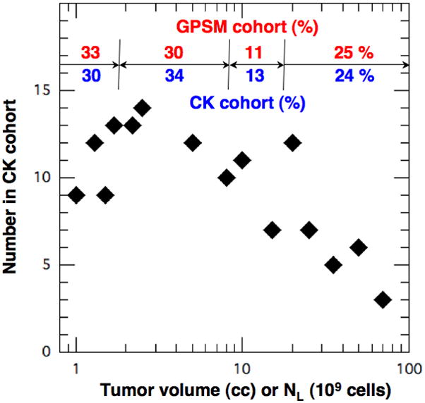
Number in patient population in Table 3 vs. the tumor volume (cc) or equivalent cell count N_L (10⁹). The percentages in the four tumor volume categories from Table 2 (red) agree with those in Table 3 (blue) within 10%.

We now construct a distribution for the second GPSM variable P by associating our TVs with PSA in a way that is consistent with Table 2 and clinical observations. In particular, Stamey et al [12] found that PSA increases with TV but with a wide variability among men (e.g. PSAD ~ 1–30μg/L-cc). As summarized in ref. [11], others found similar results for PC with a range of PSAD ~ 0.05–10 μg/L/cc. We use these observations to assign each point in Fig. 2 to one of the PSA ranges defined in the GPSM model, as shown in Fig. 3. The result is shown in Fig. 3 with an average PSAD ~ 1 μg/L/cc (dashed line) and a variability that are consistent with clinical observations. Our CK population has 15, 58, 21 and 6 % of the men in the GPSM categories P = 0, 1, 2 and 3, respectively. This is also consistent with the GPSM study, which reported only a median value of 〈PSA〉 ~ 6.4 μg/L and a range 0.2–144 μg/L.

Figure 3.

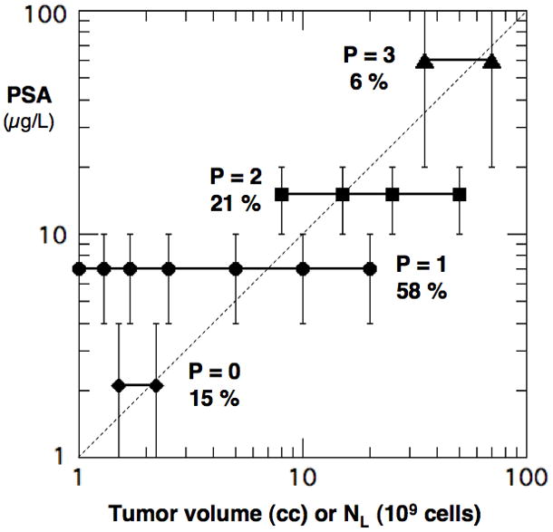
P value for each PSA group vs. the cell counts N_L (10⁹) in Table 3.

The GPSM report [1] did not include detailed distributions for regional involvement, but it did stratify for TNM and indicated that 30% had positive margins. Their tumor stage distribution was used to define our TVs according to the estimates of Dimonte [11]. Also, their margin data was used to assign 30% of the CK population to have S+M = 2. The variables S and M were not stratified separately in our CK population due to the lack of clinical data and because the GPSM model applies the same 2 points to positive margins (M) and the involvement of seminal vesicles or lymph nodes (S).

With the characteristics in Figs. 1–3, our CK population reproduces the clinical distribution of total GPSM score, as shown in Fig. 4. The diamonds represent the GPSM cohort and the histogram represents the CK population with the TVs in the legend. Both distributions are similar and exhibit a peak at GPSM = 7, which can be associated with peaks at GS ~ 6, PSA ~ 4–10 μg/L (P = 1), negative margins (M = 0), and no involvement of the seminal vesicles or lymph nodes (S = 0). The highest risk patients with GPSM ≥ 13 generally have GS = 9, P ≥ 2 and S+M ≥ 2.

Finally, to compare the CK calculations with clinical results, we must associate an individual’s sequential PSA data to his tumor volume and growth rate. The first is done by calibrating the patient’s PSA by his measured TV at biopsy or RP, namely, in terms of the cell specific PSA K (cell analog to PSAD). For example, Table 2 indicates a median 〈PSA〉 ~ 6.3 μg/L and 〈TV〉 ~ 2–7 cc for the GPSM cohort. Assuming that normal prostate cells produce an average offset of PSA_o ~ 2 μg/L, we obtain a median 〈PSAD〉 ~ (〈PSA〉− PSA_o)/〈TV〉 for PC in the range 1 μg/L/cc consistent with other observations [11, 12] and Fig. 3. Since the CK model is formulated in terms of PC cells, we use Eqs. 5–6 to convert the 〈PSAD〉 to a median cell specific PSA of

$$\langle K\rangle \sim \frac{\langle \mathit{PSA}\rangle -{\mathit{PSA}}_o}{\langle N_L\rangle }\sim {10}^{-9}\mu g/L\mathit{per}\mathit{cell}$$ (7)

with our assumed cell footprint of D³ ~ 10⁻⁹ cc. We use Eq. 7 to relate the GPSM recurrence at PSA = 0.4 μg/L to a cell count of 4 10⁸ in the CK model. It is true that TV estimates are uncertain, but a 2x uncertainty in TV corresponds to an error of one PSADT in a calculated survival time. Since the CK model yields PC survival times ~ 10–40 PSADT and the measured PSADT (=0.693 PSA/(dPSA/dt)) is independent of TV, the uncertainty in TV yields a small (≤10%) error in PC survival time (11).

3. RESULTS

Having established a CK cohort in Sec. 2.3 that reproduces the GPSM risk factor distributions in Table 2, we performed 143 CK calculations to generate BCR-free probabilities P_BCRF for comparison with the GPSM results [1]. Their multi-dimensional risk characteristics and CK results are detailed in Table 3. The first column in red lists the GS scores and the second in green lists the S+M scores. The row on top stratifies for TV and the second for the associated P values, all in blue. The individual entries in black and violet represent the values of scaled BCR time τ_rec from the CK model and will be clarified using sample CK calculations below. The scaled BCR times are converted to years using the median PSADT of the GPSM cohort and then compiled to construct P_BCRF(GPSM, t), as described below. We reproduce the GPSM probabilities by stratifying the CK model’s metastasis rate coefficient α for GS and S+M. We also compare BCR-free probabilities from five prominent nomograms [1–5] for a high-risk patient because he really needs an accurate prognosis.

To reproduce the GPSM results, we expanded our previous [11] functional dependence of α on GS to include regional involvement through M +S, as shown in Fig. 5. The dependence of α on GS was originally chosen [11] to describe the GS stratification in the PC survival studies of Freedland et al [7] and D’Amico et al [6]. However, over 90% of their patients had organ confined T1-2 tumors who were described with α ~ 3 10⁻⁵ for GS ≤ 7 and α ~ 1–6 10⁻³ for GS ≥ 8. Such values are used here for organ confined PC (M, S = 0), but larger values of α are required to describe the GPSM stratification for regional involvement (M, S ≠ 0), as shown in Fig. 5. Values of α for the intermediate risk group at GS = 7 are chosen as a geometric mean of low- and high-risk values consistent with the GPSM weighting for GS and M or S. In practice, these values of α represent averages for each risk group and may vary threefold up and down within each stratification.

Figure 5.

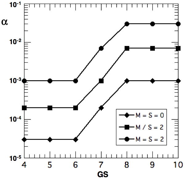
Value of CK metastasis rate coefficient α vs. GS stratified by M+S = 0, 2 and 4

Individual CK calculations are shown in Fig. 6 for a low- (A) and high-risk (B) patient in our population. Man A represents the most likely patient (peak) in our distributions in Figs. 1 and 4 with GS = 6 and GPSM = 7. Then from Eq. 1, this patient may have organ confined PC (S+M = 0) and a PSA ~ 4–10 μg/L (P = 1). The CK solution is shown in Fig. 6a for a mid-range tumor of N_L(0⁻) ~ 5 10⁹ cells just before RP (t = 0⁻). The cell populations N_L, N_HS and N_HR are plotted in black, red and blue versus the scaled time τ. RP is taken to remove the entire local population at τ = 0⁺ (i. e. N_L(0⁺) ⇒ 0). For metastasis, we use a critical population N_crit ~ 2 10⁹ cells and α = 3 10⁻⁵ for low-risk patients similar to Dimonte [11]. When N_L exceeds N_crit at τ = −1.3, the primary tumor causes N_HS and N_HR to grow explosively until N_L is removed by RP. Then, N_HS grows exponentially on its own to the recurrence value of ~ 4 10⁸ cells at τ_rec = 10.95. Figure 5b shows man B with the same size tumor but at higher risk with GS = 9, P = 1 and M+S = 4, so that GPSM = 14. This calculation uses α = 0.03 because Dimonte [11] found that patients with GS = 8–10 require large values to describe PC survival studies [6–8]. With the same values of N_crit and K, this man suffers recurrence at τ_rec = 0.98. In all cases, we require a measurement of the tumor doubling time in order to transform the scaled recurrence time τ_rec to calendar years, and this is done using PSADT.

Figure 6.

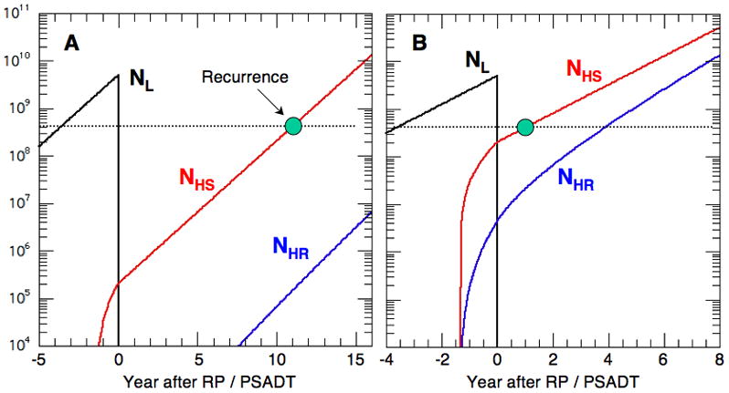
N_L, N_HS and N_HR vs. scaled time τ for N_L(0) = 5 10⁹ and (A) GS = 6, GPSM = 7, α = 3 10⁻⁵ and (B) GS = 9, GPSM = 14 and α = 0.03.

Using α(GS, M+S) from Fig. 5, we performed a CK calculation for each entry in Table 3 in order to obtain τ_rec and then construct P_BCRF(τ, GPSM) for each GPSM score. This is done by starting with P_BCRF = 1 at τ = 0 and decrementing P_BCRF at each successive τ_rec by an amount equal to the number of BCR’s divided by the total cases in that GPSM category. For example, there are 14 entries in Table 3 with GPSM = 10 (highlighted in bold and violet) using various combinations of GS, P and S+M. The first recurrence occurs at τ_rec = 2.47 for GS = 7, P = 3 (TV = 70 cc) and S+M = 0, which reduces P_BCRF to ~ 1 - 1/14 = 0.929. Then, two BCR’s occur at τ_rec = 2.58 for P = 1 (TV = 20 cc) with GS = 7 and S+M = 2 or GS = 9 and S+M = 0. These further reduce P_BCRF to ~ 0.929 - 2/14 = 0.756. Recurrence is delayed further as GS, P or S+M are reduced and a complete cure is currently taken in the CK model when TV ≤ 2 cc (i. e. N_L(0) ≤ N_crit = 2 10⁹ cells). Cures are entered as τ_rec = 100 in Table 3. Then, to compare with Fig. 1 of Thompson, et al [1], we transform τ to calendar time using the median PSADT = 1.26 yr of the GPSM cohort (t = 1.26*τ yr).

In Fig. 7, we compare values of P_BCRF from the CK model (+ with bold lines) with those from Fig. 1 of the GPSM study [1] (⋄ with thin lines) for selected values of GPSM. We consolidated the cases with GPSM = 5, 6 and 7 into one to improve statistics since their results are similar and also for GPSM = 8 and 9. The agreement is excellent and certainly within the statistical uncertainties. Those with GPSM ≤ 7 are dominated by GS ≤ 6 and their P_BCRF requires an α in the range of 10⁻⁵-10⁻⁴. Patients with GPSM ≥ 13 have GS ≥ 8 and require an α in the range of 10⁻³-10⁻². They tend to recur early and P_BCRF decreases to ~0.5 in one PSADT ~ 1.26 yr. The intermediate values of α for GS ~ 7 are chosen to simply geometrically bridge the low- and high-risk patients. The agreement in Fig. 7 is excellent but the comparison is not definitive because the assumed patient characteristics in Table 3 conform to those in the GPSM cohort only in a statistical sense, as shown in Figs. 1 and 4. Nevertheless, the inferred values of α in Fig. 5 are consistent with those required to fit clinical PC survival studies [6–8].

Figure 7.

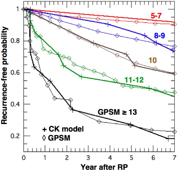
BCR-free probability vs. time after RP for various GPSM scores. Bold lines (+) are from the CK model and thin lines (◇) are from Fig. 1 of Thompson et al [1].

The excellent agreement in Fig. 7 and with PC survival studies requires not only a viable model but also a faithful reproduction of the patient population. For example, Lughezzani et al [9] found that BCR nomograms have a limited ability to describe independent cohorts, with concordance indices of 67–74% at 5 yrs. This is troubling to a high-risk individual who needs an accurate prognosis and whose risk factors may not project well to the distribution in a particular cohort. The dilemma is exemplified in Fig. 8 for a 62 year old patient who had RP in 1998 with PSA ~ 7 μg/L, GS = 9, TV = 5 cc with 50% positive biopsy cores, T3b stage, positive margins and seminal vesicle involvement. The GPSM model (red) with a score of 14 yields the P_BCRF that decreases dramatically in time. The CK result (black dash) is similar using the median PSADT = 1.26 yr of the GPSM cohort. The CAPRA model (magenta) with a score of 7 reproduces the initial rapid decline in P_BCRF but reaches the smallest value of P_BCRF ≤ 0.1 at 5 yrs. The D’Amico (high-risk, orange) and Han (green) models all decline more slowly initially and approach the GPSM result later in time. The MSKCC model (blue) decreases most slowly and remains high at 10 yr with P_BCRF ~ 0.33. This value would be even higher P_BCRF ~ 0.47 for RP performed in 2010.

Figure 8.

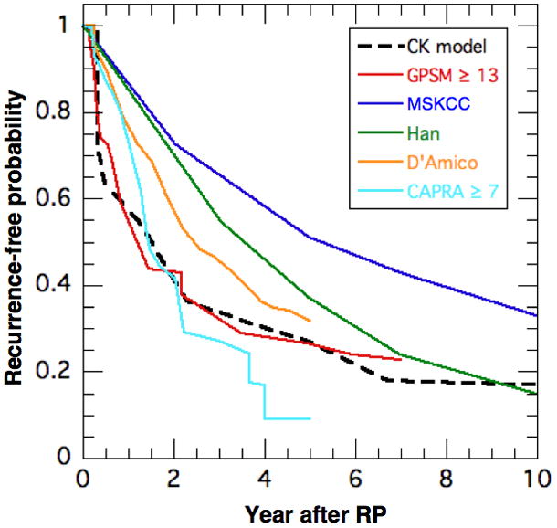
Biochemical recurrence-free probability vs. time for CK (black), GPSM (red), MSKCC (blue) and Han (green) models. The MSKCC values are for RP in 1998 since the GPSM values are for 1997–2001. (RP in 1998 at age = 62 yrs, PSA = 7 μg/L, GS = 9, T3b, positive margins and seminal vesicle involvement)

The differences among the nomograms are troubling for this most-vulnarable, high-risk patient and his attending physician. As seen in Table 4, P_BCRF varies almost six fold at 5 years, from 9% for the CAPRA model to 51% for the MSKCC model for RP in 1998. The time to median probability of BCR (P_BCRF = 0.5) also varies significantly from around 1.4 yr for the GPSM, CK and CAPRA models to 2.4, 3.6 and 5.1 yr for the D’Amico, Han and MSKCC models, respectively. Please note that some of this variation could be due to the differences in the BCR endpoint definitions summarized in Table 4. It is also noteworthy that most patient populations have relatively few high-risk patients. Needless to say, it would be helpful to reduce these uncertainties by developing a more universal and personalized model that includes tumor dynamics.

Table 4.

Probability of BCR survival (%) after RP from various nomograms for the high-risk patient in Fig. 8 (RP in 1998 at age = 62 yrs, PSA = 7 μg/L, GS = 9, T3b, positive margins and seminal vesicle involvement). The CK model transformed τ to calendar time using the median PSADT = 1.26 yr of the GPSM cohort. The time to median P_BCRF (= 50 %) is given in years after RP. The BCR condition is given in the last column for each model.

NOMOGRAM	Probability of BCR survival (%)				Years to 50% PBCRF	BCR PSA (μg/L)
	2 yr	5 yr	7 yr	10 yr
CK model	42	27	18	17	1.5	≥ 0.4
GPSM (≥ 13)	43	27	23	-	1.2	≥ 0.4
MSKCC (1998)	73	51	43	33	5.1	≥ 0.4 × 2
Han	70	37	24	15	3.6	≥ 0.2
D’Amico high-risk	58	32	-	-	2.4	3 rises
CAPRA (≥ 7)	42	9	-	-	1.4	2 consec. ≥ 0.2

4. CONCLUSIONS

Nomograms from leading medical institutions were found to yield very different BCR-free probabilities (P_BCRF) for a high-risk patient, as shown in Fig. 8 and Table 4. We consider three possible sources for these differences. First, each nomogram is optimized by regressions to a cohort with a particular distribution of risk factors, which may differ from those of other cohorts. For example, even though the MSKCC [2] and GPSM [1] studies both had median values of PSA ~ 6.5 μg/L and GS ~ 6, the former had 40–50% of their patients with T1 stage and ~1% requiring adjuvant therapy whereas the latter had none with T1 and ~12% requiring adjuvant therapy. The universality of a nomogram can best be clarified by choosing a validation cohort whose distribution of risk factors differs from that of the parent cohort. For example, the modeling and validation cohorts for the MSKCC model [2] had similar values of median PSA ~ 6–6.6 μg/L, GS ~ 6–7 and T1c-T2a stage; so it is not surprising that the concordance between the two cohorts is good. Second, the nomograms assign different scores to similar risk factors. For the high-risk patient in Fig. 8, GS accounts for 64% of the GPSM score and 27% of the MSKCC score whereas PSA contributes 7% and 49%, respectively. In addition, the GPSM and MSKCC models stratify for margins and seminal vesicles whereas the Han Table combines them into one regional category. Third, the risk factors in the current nomograms are stratified for the state of the tumor at diagnosis but not its growth rate. This is problematic because two patients with identical PSA, GS, tumor stage (volume) and regional involvement at the time of surgery would have identical BCR-free probabilities in each model (although P_BCRF would vary among models). Yet, PC recurrence [10] and survival [6–8] studies show that progression times depend on PSADT, which implies that the differences in Fig. 8 and Table 4 could be reduced if the nomograms stratify for PSADT (although hard to measure pre-operatively). This also important because the differences in BCR endpoints, as summarized in Table 4, translate to 1 PSDAT variation in the time to BCR for each twofold difference in the PSA endpoint for BCR.

The clinical implication of these results is that a newly diagnosed patient obtains different prognoses from the various nomograms because his PC risk factors are weighted differently, and without distinction between slow- and fast-growing tumors. To complement outcome probabilities from a particular cohort, the patient and his attending physician may want a personalized time-dependent PC model that utilizes the individual’s diagnosed tumor state and growth rate.

To this end, Dimonte [11] developed a CK model for an individual prognosis that was able to describe PC survival studies [6–8], which stratified for GS, PSADT and time to recurrence after RP. Since more clinical data exist on recurrence and BCR is a pre-cursor to PC specific mortality, we tested the CK model here against the GPSM model and its large, well-stratified cohort from the Mayo Clinic. In particular, Table 2 describes the GPSM cohort not only in terms of GS, PSA, and regional invasion, but also by tumor volume and PSADT. Since the GPSM model describes a patient cohort while the CK model applies to individuals, we first constructed a CK cohort of 143 men that has the same risk-factor distributions as the GPSM cohort (Sec. 2.3). We then used the calculated CK results to construct BCR-free probabilities, which agree with the observed P_BCRF(t, GPSM) for all GPSM scores, as shown in Fig. 7. This comparison expands the stratification of the CK model’s metastasis rate coefficient α beyond GS to include regional involvement (S+M), as shown in Fig. 5. Such a comparison could be performed with the other nomograms if they stratified their cohorts for TV and PSADT, as needed by the CK model.

The clinical goal is to complement nomograms with the CK model to quantify an individual’s PC progression from diagnosis through therapy, and possible BCR, confirmed metastatsis and PC specific death. To date, we used population-based studies on recurrence [1] and PC specific death [6–8] to develop and test the CK model, with excellent results in Fig. 7 and ref. [11]. However, before clinical use, the CK model must be tested more stringently by modeling a variety of individual patients with comprehensive diagnostic data and calibrated serial PSA measurements from diagnsosis to death. This is currently under study with high-risk patients from the Mayo Clinic.

Abbreviations and Acronyms

α

Model coefficient for cell metastasis rate relative to PSADT

F_x

Forcing functions in Eqs. 3 for cell population x = L, HS, HR

GS

Gleason score

HT

Hormone Therapy

K

Cell specific PSA = PSA/cell for cancer cells

N_crit

Critical number of LOCAL cells (N_L) required to start metastasis

N_HS

Number of PC cells in HORMONE SENSITIVE population

N_HR

Number of PC cells in HORMONE RESISTANT population

N_L

Number of PC cells in LOCAL population

N_Lmax

Maximum number of cells at which N_L saturates

N_PCD

Number of cells required to cause PC specific death

PC

Prostate cancer

PSA

Serum prostate specific antigen in μg/L = ng/mL

PSA_o

PSA offset associated with normal prostate cells

PSAD

PSA density = PSA per tumor volume in μg/L/cc

PSADT

PSA doubling time

P_BCRF

Probability of biochemical recurrence-free survival

RP

Radical prostatectomy

RT

Radiation therapy

T_rec

Time for PSA to recur after RP

τ

Time t scaled by PSADT

References

- 1.Thompson RH, Blute ML, Slezak JM, Bergstralh EJ, Leibovich BC. Is the GPSM scoring algorithm for patients with prostate cancer valid in the contemporary era ? J Urology. 2007;178:459–463. doi: 10.1016/j.juro.2007.03.124. [DOI] [PubMed] [Google Scholar]
- 2.Stephenson AJ, Scardino PT, Eastham JA, Bianco FJ, Dotan ZA, DiBlasio CJ, Reuther A, Klein EA, Kattan MW. Postoperative nomogram predicting the 10-year probability of prostate cancer recurrence after radical prostatectomy. J Clin Onc. 2005;23:7005–7012. doi: 10.1200/JCO.2005.01.867. (Nomogram can be found at www.mskcc.org/applications/nomograms/prostate/PostRadicalProstatectomy.aspx) [DOI] [PMC free article] [PubMed] [Google Scholar]
- 3.Cooperberg MR, Pasta DJ, Elkin EP, et al. The University of California San Francisco Cancer of the Prostate Risk Assessment score: a straightforward and reliable pre-operative predictor of disease recurrence after radical prostatectomy. J Urol. 2005;173:1938–42. doi: 10.1097/01.ju.0000158155.33890.e7. [DOI] [PMC free article] [PubMed] [Google Scholar]
- 4.Han M, Partin AW, Zahurak M, Piantadosi S, Epstein JI, Walsh PC. Biochemical (PSA) recurrence probability following radical prostatectomy for clinically localized prostate cancer. J Urology. 2003;169:517–523. doi: 10.1097/01.ju.0000045749.90353.c7. (Nomogram can be found at http:/urology.jhu.edu/prostate/hanTables.php) [DOI] [PubMed]
- 5.D’Amico AV, Whittington R, Malkowitz SB, et al. Biochemical outcome after radical prostatectomy, external beam radiation therapy, or interstitial radiation therapy for clinically localized prostate cancer. JAMA. 1998;280:969–74. doi: 10.1001/jama.280.11.969. [DOI] [PubMed] [Google Scholar]
- 6.D’Amico AV, Moul JW, Carroll PR, Sun L, Lubeck D, Chen MH. Surrogate end point for prostate-cancer specific mortality after radical prostatectomy or radiation therapy. J Nat Can Inst. 2003;95:1376–1383. doi: 10.1093/jnci/djg043. [DOI] [PubMed] [Google Scholar]
- 7.Freedland SJ, Humphreys EB, Mangold LA, Eisenberger MA, Dorey FJ, Walsh PC, Partin AW. Risk of Prostate Cancer-specific mortality following biochemical recurrence after radical prostatectomy. JAMA. 2005;294:433–439. doi: 10.1001/jama.294.4.433. [DOI] [PubMed] [Google Scholar]
- 8.Armstrong AJ, Garrett-Mayer ES, Yang YC, deWit R, Tannock IF, Eisenberger MA. A contemporary prognostic nomogram for men with hormone-refractory metastatic prostate cancer: a TAX327 study analysis. Clin Cancer Res. 2007;13:6396–6403. doi: 10.1158/1078-0432.CCR-07-1036. [DOI] [PubMed] [Google Scholar]
- 9.Lughezzani G, Budaus L, Isbarn H. Head-to-Head Comparison of the Three Most Commonly Used Preoperative Models for Prediction of Biochemical Recurrence After Radical Prostatectomy. Euro Urol. 2010;57:562–568. doi: 10.1016/j.eururo.2009.12.003. [DOI] [PubMed] [Google Scholar]
- 10.Freedland SJ, Humphreys EB, Mangold LA, Eisenberger M, Partin AW. Time to Prostate Specific Antigen Recurrence After Radical Prostatectomy and Risk of Prostate Cancer Specific Mortality. J Urology. 2006;176:1404–1408. doi: 10.1016/j.juro.2006.06.017. [DOI] [PubMed] [Google Scholar]
- 11.Dimonte Guy. A cell kinetics model for prostate cancer and its application to clinical data and individual patients. J Theoretical Biology. 2010;264:420–442. doi: 10.1016/j.jtbi.2010.02.023. [DOI] [PubMed] [Google Scholar]
- 12.Stamey TA, Yang N, Hay AR, et al. Prostate-Specific antigen as a serum marker for andenocarcinoma of the prostate. New Eng J Med. 1987;317:909–916. doi: 10.1056/NEJM198710083171501. [DOI] [PubMed] [Google Scholar]
- 13.Bostwick DG, et al. Staging of early prostate cancer: a proposed tumor volume-based prognostic index. Urology. 1993;41:403–411. doi: 10.1016/0090-4295(93)90497-x. [DOI] [PubMed] [Google Scholar]
- 14.Dattoli G, Guiot C, Delsanto PP, Ottaviani PL, Pagnutti S, Deisboeck TS. Cancer metabolism and the dynamics of metastasis. J Theoretical Biology. 2009;256:305–310. doi: 10.1016/j.jtbi.2008.10.008. [DOI] [PubMed] [Google Scholar]