Efficiently identifying genome-wide changes with next-generation sequencing data

Abstract

We propose a new and effective statistical framework for identifying genome-wide differential changes in epigenetic marks with ChIP-seq data or gene expression with mRNA-seq data, and we develop a new software tool EpiCenter that can efficiently perform data analysis. The key features of our framework are: (i) providing multiple normalization methods to achieve appropriate normalization under different scenarios, (ii) using a sequence of three statistical tests to eliminate background regions and to account for different sources of variation and (iii) allowing adjustment for multiple testing to control false discovery rate (FDR) or family-wise type I error. Our software EpiCenter can perform multiple analytic tasks including: (i) identifying genome-wide epigenetic changes or differentially expressed genes, (ii) finding transcription factor binding sites and (iii) converting multiple-sample sequencing data into a single read-count data matrix. By simulation, we show that our framework achieves a low FDR consistently over a broad range of read coverage and biological variation. Through two real examples, we demonstrate the effectiveness of our framework and the usages of our tool. In particular, we show that our novel and robust ‘parsimony’ normalization method is superior to the widely-used ‘tagRatio’ method. Our software EpiCenter is freely available to the public.

INTRODUCTION

High-throughput next-gen sequencing (NGS) technologies, while emerging only 5 years ago, have already been widely used for biomedical research and discovery. Cost-effective NGS has almost completely replaced the traditional Sanger sequencer in genome sequencing and re-sequencing for discovery of genetic variation. NGS has also extended sequencing applications to far broader fields: studying DNA–protein interactions and gene regulation, identifying novel transcripts or splice isoforms and detecting differentially expressed genes. Indeed, the most powerful and popular sequencing-based methods, ChIP-seq and mRNA-seq, are increasingly replacing microarray as the standard method in these applications. In comparison with microarray-based methods, these NGS-based methods offer not only digital readings, larger dynamic signal range and higher reproducibility but also capabilities such as discovering novel transcripts and studying mRNA polymerase II pausing (1).

The promising biomedical applications of NGS have spurred the development of computational tools for analyzing NGS data. Tools already available for analyzing ChIP-seq data from genome-wide studies of transcription factor binding sites (TFBS), a popular early application of NGS, include: QuEST (2), MACS (3), FindPeaks (4), CisGenome (5), SISSRs (6), PeakSeq (7) and PICS (8). These tools identify small genomic regions (e.g. 50–300 bp) with significant enrichment of sequencing read tags and predict the location of binding sites as the peak of read tags. A recent review by Mortazavi et al. (9) and a comparison study by Laajala et al. (10) provide a more complete list of tools and summarize their capabilities and performance. Other main applications of ChIP-seq include genome-wide surveys of histone acetylation or methylation patterns, and identification of differential epigenetic modifications of histones between different cell types. Unlike transcription factors, histone proteins are core components of DNA chromatin. Epigenetic modifications of histones typically happen over much larger genomic regions and often lack the characteristic peak distribution of TFBS. While histone ChIP-seq is becoming an important and popular method for epigenetic studies, only a few tools [e.g. ChIPDiff (11) and ChromaSig (12)] are currently available for analyzing such data.

Another widely used NGS application, mRNA-seq, can detect novel transcripts, identify differentially expressed genes, locate full length of transcripts and even map out the whole transcriptome (13,14). In addition, mRNA-seq is being used to interrogate post-transcriptional gene regulation including the control of alternative splicing (15) and polyadenylation (16), RNA editing (17) and degradation and translation of mRNA. Recent reviews (1,9) highlight the importance and advantages of mRNA-seq for these applications. Several tools have been developed for mRNA-seq data analysis: TopHAT (18), RNA-Mate (19) and QPALMA (20) are specialized for aligning reads of mRNA sequences to their genome reference; ABySS (21) and Velvet (22) are for de novo assembly of mRNA sequences when a genome reference is either not available or of low quality; ERANGE (23), RSAT (24), BASIS (25) and Cufflinks (26) assess abundance of mRNA transcripts; edgeR (27), DESeq (28) and DEGseq (29) detect differentially expressed genes. Despite this progress, the development of data analytic methods lags behind the recent increase in mRNA-seq applications (30).

We propose a new statistical framework of hypothesis testing for the comparative analysis of both ChIP-seq and mRNA-seq data. Our framework is designed to detect genomic regions that differ between cell types or experimental conditions (denoted as samples) in the density of epigenetic markers (ChIP-seq applications) or in the abundance level of gene transcripts (mRNA-seq applications). In addition, we introduce several normalization methods, including our novel ‘parsimony’ method, for adjusting differences in read coverage depth between samples. Our ‘parsimony’ method, unlike any traditional method, can automate data normalization and shows performance superior to other methods in our examples. To achieve a low false discovery rate (FDR), our framework employs a sequence of three tests: the first filters outs background regions, and the second and third tests act together complementarily in identifying significant changes. The second test, the exact rate ratio test, uses ‘un-normalized’ read counts to determine whether differences between samples exceed the expected Poisson variation, assumed to arise mainly from random experimental processes. The third test, the z-test, uses log2 ratio data of normalized read counts to decide whether such differences exceed the combination of Poisson and other extra variation, assuming the extra variation is mainly derived from random biological processes (see Supplementary Figure S1 for illustration). In addition, we introduce a new software tool EpiCenter that implements our statistical framework and is freely available to public at http://www.niehs.nih.gov/research/resources/software/epicenter. This tool has also been successfully used to analyze several histone ChIP-seq and mRNA-seq data from multiple studies (31).

METHODS

Read filtering and noise reduction

To filter poorly aligned reads and those mapped to multiple positions, EpiCenter takes advantage of the read alignment quality scores reported by mapping tools such as MAQ, or ELAND. These alignment tools assign low scores to reads that have multiple mismatches (poorly aligned reads) or that can be aligned to multiple positions in a genome. By default, EpiCenter filters out any reads with alignment quality scores lower than 10, to exclude reads mapped to repetitive regions and reads aligned poorly. Users can set the quality-score cutoff to tailor the read alignment filter for their specific applications.

Another main source of noise in sequence reads arises from non-specific binding sequences from ChIP experiments or other random sequences from DNA sample preparation. These noise reads are likely to be randomly distributed across the genome in the sense that their locations follow a Poisson process. Let_. be the expected rate of random hits of read tags across the entire genome in sample k, where . Under the assumption that all reads are random noise, can be estimated as

where L is the length of genome reference sequence, and C_k is the total number of mapped reads in the k-th sample. EpiCenter uses this estimate by default but allows the user the option of specifying directly. For a two-sample comparison, if users specify only , EpiCenter will automatically estimate as , and vice versa.

Besides this noise-rate-based filtering method, EpiCenter also offers a way to filter out background regions by a user-defined cutoff of an absolute number of read tags. For example, users can filter out all regions with fewer than 10 tags.

Procedures for estimating the read rate ratio and for data normalization

Background

Variability is introduced in all steps of a sequencing experiment and leads to variation in read counts or coverage depth between different samples, variation that is unrelated to the biological questions under investigation. The sources of experimental variation include the amount of input DNA in sample preparation and data quality from different sequencing lanes and machines. In addition, one experimental condition can have higher overall read counts than another simply because it was sequenced more. To make comparisons fair, a test statistic must account for such experimental variation that can change expected read counts. Our exact rate ratio test does so by adjusting the expected read rate ratio under the null hypothesis instead of by normalizing the raw read count data themselves. Our z-test, however, uses normalized read counts to account for such experimental variation and biological variation. We developed several methods, appropriate in different scenarios, for estimating the expected read rate ratio or for normalizing data. All these methods are essentially data normalization procedures.

For all procedures, we divide a genome of length L into non-overlapping windows (e.g. 1 kb windows). Assume that we have n non-overlapping windows, and let and be the random variables associated with the raw counts of read tags in window i from Samples 1 and 2, respectively. Also, let and be the corresponding normalized counts. Let E be the expectation function, and be the ratio of expected rates for read counts in Sample 2 over that in Sample 1. We assume that is constant across different windows indexed by i and that read-tag counts in the window i follow a Poisson distribution with parameters λ_ki in sample k. Since we assume that and are all independent for , and , also follows a Poisson distribution with parameters . The null hypothesis is that the Poisson rates are the same for both samples after appropriate normalization, that is, . Consequently, using these facts we can write:

From the rightmost equality, we have that

The above equation can be extended to scenarios with more than two samples, say . In such cases, we use R_k/1 to represent the ratio of expected rates of reads in sample k over Sample 1. Therefore, under these assumptions, the only unknown for read count normalization is R_k/1. We have developed several approaches to estimate it.

TagRatio method

The first approach, called the tagRatio method, is the most commonly used in published work and is appropriate when the sequencing noise level is similar across samples. The estimate of R_k/1 is simply the ratio of total number of mapped read tags from the two samples, namely:

This estimator works best when any biological difference between the samples has negligible effect on the overall number read tags as, for example, when an increase in read tags in some regions is approximately balanced by a decrease in others.

Parsimony method

We also developed a novel and unconventional data normalization method that we call the ‘parsimony’ approach; the term was borrowed from the parsimony method for phylogenetic tree reconstruction in evolutionary biology. The parsimony method of tree building reconstructs a phylogenetic tree by minimizing the number of DNA base changes of related species. Following that idea, our ‘parsimony’ normalization method finds the best estimate of R_k/1 as the one that minimizes the number regions/genes that the exact rate ratio test declares statistically significant between two samples. The key assumption is that biological organisms always minimize changes of genome or overall gene expression pattern when adjusting to new genetic/environmental changes. This assumption implies that majority of regions/genes should not change between samples. Different from the other methods mentioned above, the ‘parsimony’ method does not estimate the expected ratio of Poisson rates before statistical testing; instead, it uses the exact rate ratio test recursively to find the optimum ratio.

Methods based on selection of unchanged regions

A third general approach is, instead of using all mapped read tags, to select genomic regions that are believed to have no biological differences and to use only read counts from these putative ‘unchanged’ regions for normalization. Ideally, one uses regions that are known from previous work to be the same between samples. Without such a priori knowledge, one could select genomic regions where both samples have substantial read counts. The idea is to avoid any region with low counts where a small change in count for either sample can dramatically alter sample-specific ranks and their ratio of read counts between the two samples. Alternatively, EpiCenter employs a rank-based approach to select putatively unchanged regions. After ranking genomic regions separately by their observed counts for each sample, EpiCenter selects, as ‘unchanged’, any regions that fall into a particular range of ranks. The choice of an appropriate range of ranks can still be tricky though: if the range is too small, there may be too few regions included to get a good estimate; if the range is too large, regions declared ‘unchanged’ may be contaminated with some harboring real changes. We suggest leaving out the top-ranked 5% of regions as they are more likely to be repetitive regions with extremely high depth of read coverage. For example, one might select regions that, when ranked separately in each sample, fall between the 90 and 95 percentiles of read counts in both samples. By selecting top-ranked non-repetitive regions, we reduce the impact of both the Poisson variability in read counts, and the uncertainty in mapping read tags to repetitive regions on the estimation of R_k/1.

Using these ‘unchanged’, therefore presumed null, genomic regions, we estimate the expected rate ratio as the slope of a linear least-squares regression line through the origin (i.e. intercept set to 0) fitted to pairs of read counts . In addition, EpiCenter reports both the mean and median of as alternative estimates. The median estimate is more robust to extreme ratios in a few genomic regions than either the mean or linear least-squares estimate of .

Choice among methods deciding which procedure might be the best for estimation of R_k/1 or for data normalization may be difficult. Methods based on selection of unchanged regions require either prior knowledge of such regions (rarely available in practice) or a trial-and-error approach where performance could suffer. Consequently, we focus on the ‘tagRatio’ and ‘parsimony’ methods here. Based on our observations from real and simulated data, if we filter out low read count regions, the log2 ratios of normalized read counts from those regions declared to be non-significant by the exact rate ratio test has approximately a Gaussian distribution. We use this observation to motivate our proposed z-test. So, one way to compare data normalization procedures is just to assess how well the distribution of log2 ratios from non-significant regions approximates a Gaussian distribution.

Significance tests

Background filtering test

EpiCenter carries out a sequence of three significance tests. The first test is applied to all genomic regions to filter out any regions where read tags do not have significantly more counts than expected from random Poisson background noise in all experimental conditions. This test is done region by region separately for each condition, and the data are the total raw read counts in each region. Under the assumption that read counts across the whole genome follow a Poisson distribution, the P-value for region i in sample k, , is given by:

where Q is the cumulative distribution of function of the Poisson distribution, alternatively known as a regularized gamma function, is the raw read count in a genomic region i of length in sample k. The P-value is the probability of observing or more reads in a genomic region given the sample-specific noise rate . A genomic region is retained for further consideration if this filter indicates that the observed counts in the region are enriched above the background noise for at least one sample, that is, < 0.05 for at least one sample. Note that the test will not apply if users choose the noise filter that is based on a user-defined cutoff of an absolute number of read tags.

The exact rate ratio test

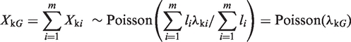
The second statistical test in our sequence is applied only to those genomic regions that pass the initial background filter. EpiCenter uses the exact rate ratio test to determine whether observed difference in read counts between samples can be explained by experimental variation. This test statistic assumes that read counts in a genomic region follow the Poisson distribution, and Poisson rates of different regions within a sample can be different. Additionally, it assumes that read counts from different samples are independent. Let G be a genomic region or gene that consists of m (biologically) uniform regions. A uniform region is defined as a contiguous region that is expected to be uniform in read coverage. So Poisson rates of read tags are the same at all positions within each uniform region but can be different between regions.

Now let X_ki represent a uniform genomic region covering l_i bases. According to the two assumptions above, , which means that is distributed as a Poisson random variable with per base rate . We also have

where . For example, in the two-sample case, we have , , and and are independent. To see whether the genomic region G is differentially changed between the two samples, we would usually test the null hypothesis that or, equivalently (given ). However, different samples may vary in read coverage simply because they differ in number of sequencing lanes, quality of sequences or sequencing machines. Consequently, instead of normalizing read counts, we test the null hypothesis , where R_2/1 is estimated as described above. Because and are two independent Poisson random variables, the distribution of given is a binomial distribution, i.e., , or, under our null hypothesis, . Based on this theory, we construct the exact binomial test statistic for testing the null hypothesis that . We call this test the exact rate ratio test. This approach can be extended to cases with more than two samples by making pairwise comparisons.

z-test of log2 ratios

The third statistical test in our sequence is designed to find those genomic regions or genes whose rate ratio (or fold change) between samples is extreme in comparison to the expected distribution of rate ratios across the genome. The second test determined which regions have different Poisson rates between two samples, but its adjustment for different overall rates between samples via does not fully allow for biological variation or other extra variation. Simply comparing P-values from that test across genomic regions has drawbacks because genomic regions with high depth of coverage will have smaller P-values than regions of low depth of coverage even if ratio of Poisson rates is the same for both regions. To take fuller account of extra variability in estimated rate ratios, we take as data the log2 ratios of read counts in the two samples and construct a z-test by assuming a Gaussian distribution for the log2 ratio. We present the z-test here for two samples, but it can be applied to any pairwise comparison if there are more than two samples. The log2ratio of read tags between two samples j and k in genome region i, denoted , is defined as:

where and denotes the normalized read counts in the same region i from sample j and sample k, respectively. The test is motivated by the key observation from real ChIP-seq and mRNA-seq data that the distribution of the log2 ratios between two samples closely approximates a Gaussian distribution, after filtering out genomic regions of low read count (<10) and regions changed significantly (as declared by the exact rate ratio test), which is illustrated in two real-data examples. We also supported this observation using simulations generated under a broad range of Poisson rates of read tags and the degree of extra biological variation (see ‘Materials and Methods’ for simulation procedures). The simulation showed that in both scenarios with or without biological variation, the log2ratio distributions of read counts between two samples, after filtering our low read count regions, closely approximate a Gaussian distribution (see Figure 1 for examples). Since the expected value of of unchanged regions is 1, the distribution of under our null hypothesis has mean zero. Our z-test takes, as its null distribution, a Gaussian distribution with mean zero and an estimated standard deviation. Depending on available data, we suggest different methods for estimating the standard deviation (see Supplementary Figure S2). When biological replicates are not available, EpiCenter estimates by default the standard deviation of this null distribution, after filtering out regions with <10 read tags, from regions declared to be non-significant by the exact rate ratio test. The null standard deviation can also be specified by users as an option.

Figure 1.

The null distribution of log2ratio of simulation data. The plot shows histograms of log2 ratio of read counts between two independent samples. The red dotted line in each histogram is the Gaussian approximation to the histogram. The simulation data were generated under different Poisson rates with/without imposing biological variation: (A) read simulated under one Poisson rate (0.01) and no biological variation; (B) read simulated under the Poisson rate 0.1 and no biological variation; (C) read simulated under the Poisson rate 1 and no biological variation; (D) read simulated under different Poisson rates (rates ranging from 0.01 to 10) and different levels of biological variation (SD ranging from 0 to 0.3). The simulation results show that the log2ratio of read counts can be well approximated by the Gaussian distribution when the average number of read tag per regions is >10.

Determining significance of change

The exact rate ratio test and the z-test are different, and thus one test can indicate that a region is significantly changed between samples whereas the other may not. The exact rate ratio test tends to have a high false positive rate when biological or other variation contributes substantially to read count difference between samples. The exact rate ratio test is especially sensitive when read counts are large. The z-test is more robust against extra variation, but does not work well when read counts are low. In this sense, the two tests are complementary. Consequently, we combine results from both tests by taking the maximum P-value, denoted as Max-P, from the two tests for each region, and use its value to determine whether the region is significant.

Simulation analysis of log2ratio null distribution

We used simulation to investigate whether the null distribution of the log2ratio approximates a Gaussian distribution. We simulated read counts of mRNA-seq data for two independent samples. Each simulated data set included 10 000 independent genes, each of length 1000 bp, and read counts were simulated for two independent samples under two scenarios: (i) read count data having only Poisson variation by mimicking only experimental variation, and (ii) read count data containing both Poisson variation and additional variation by mimicking both experimental variation and biological variation. For the first scenario, read counts of two samples were generated from an identical Poisson distribution, and we simulated 20 data sets, each with different Poisson rates: 0.01, 0.03, 0.05, 0.07, 0.09, 0.1, 0.3, 0.5, 0.7, 0.9, 1, 2, 3, 4, 5, 6, 7, 8, 9 and 10. For the second scenario, we simulated a total of 200 data sets, each under a combination of the same 20 Poisson rates and 10 levels of extra variation (mimicking biological variation) in log2ratio as governed by Gaussian distributions with mean 0 and 10 levels of standard deviation: 0.01, 0.03, 0.05, 0.07, 0.09, 0.1, 0.2, 0.3, 0.4, 0.5. For each data set in the second scenario, we simulated read counts through the following three main steps: first, we generated gene-specific 10 000 log2ratios at random from a Gaussian distribution of mean 0 and a given standard deviation; second, for each gene for the first sample, we generated a random Poisson read count using a given Poisson rate and third, for each gene in the second sample, we used its gene-specific log2ratio and the given Poisson rate to calculate the adjusted Poisson rate applicable to the gene. We then used the adjusted Poisson rate to generate an independent Poisson read count for the gene. In both simulation scenarios, all genes whose maximum read count in both samples was less than 10 were removed from each simulated data set before estimating the null distribution of log2ratio.

Data simulation for performance assessment

We assessed the performance of our method in a simulation study involving 9500 unchanged and 500 differentially expressed genes, each of length 1000 bp. The fold changes of the 500 differentially expressed genes were uniformly distributed between 1.5 and 10. We modeled different depths of read coverage with 15 different Poisson rates: 0.1, 0.3, 0.5, 0.7, 0.9, 1, 2, 3, 4, 5, 6, 7, 8, 9 and 10 tags per genomic position. We modeled nine levels of extra variation as biological variation in log2ratio with nine zero-mean Gaussian distributions of different standard deviations: 0 (no extra variation), 0.01, 0.03, 0.04, 0.05, 0.07, 0.09, 0.1 and 0.2. We simulated read counts independently for two samples, each with two independent ‘biological’ replicates. In total, we generated 135 data sets, each under one of the possible combinations of 15 levels of read coverage and 9 levels of extra variation. We analyzed each data set independently. Using the Bonferroni correction for multiple testing, we set the cutoff P-value for statistical significance for our Max-P statistic to 5 × 10⁻⁶. For each combination of read coverage and extra variation, we calculated the false positive rate (FPR) as the proportion of the 9500 unchanged genes rejected by the test, the false negative rate (FNR) as the proportion of the 500 differentially expressed genes not rejected by the test, and the FDR as the ratio of the number of genes rejected among the 9500 unchanged genes to the total number of genes rejected. We repeated each simulation eight times, and reported the average of each measure.

RESULTS

We developed a new statistical framework as detailed in the ‘Methods’ section for the analysis of NGS data analysis. We also built a versatile new software tool, EpiCenter, to allow researchers to customize their analyses of both ChIP-seq and mRNA-seq data (Figure 2). EpiCenter can identify epigenetic changes in the whole genome or in selected genomic regions (e.g. promoters), detect differentially expressed genes using either genomic sequences or cDNA sequences and locate TFBS. EpiCenter can also convert ChIP-seq or mRNA-seq data into a simple data matrix of read counts, allowing direct use of some existing tools for data analysis. For example, users can convert multiple-sample mRNA-seq data into a single matrix of read counts and use Cluster (32) and TreeView (33) for clustering analysis and visualization. In addition, EpiCenter can generate compressed or uncompressed WIG data files for visualization in the UCSC genome browser and supports multiple major read alignment formats such as MAQ (34), ELAND, SAM and BAM. EpiCenter is computationally efficient, with typical running time <10 min and peak memory usage <4 GB. The running times for both examples of real-data applications below were <5 min on 64-bit Linux with 2.93 GHz Intel Xeon CPU. The test data and codes are available at http://bioinformatics.joyhz.com/epicenter.

Figure 2.

Illustration of EpiCenter’s approach for two-sample mRNA-seq or ChIP-seq data analysis.

Performance on simulated data

We used simulations to assess EpiCenter’s performance based on the Max-P statistic (see ‘Materials and Methods’ for details of simulation). The simulation generated 135 independent data sets of 10 000 independent genes, among which 500 were differentially expressed between the two treatment samples. Each data set, having two replicates for each of two samples, involved different depths of read coverage (overall Poisson rates) or degrees of extra variation in log2ratio between conditions. For each data set, we performed two separate analyses: one using only a single replicate (i.e. without replicates), and the other using both replicates (i.e. with replicates). Without replicates, EpiCenter first selected ‘unchanged genes’ by the exact rate ratio test, then estimated the standard deviation of the log2ratios from these ‘unchanged genes’. The P-value cutoff for the exact rate ratio test was 0.01, adjusted by the Bonferroni’s correction. With replicates, EpiCenter took, as the estimated standard deviation of log2ratios, the average of the standard deviations of two replicates of each sample. We calculated FPRs, and FNRs and FDRs from each analysis, and reported the mean of each measure under each simulation combination.

Replicates improved the performance of the Max-P statistics compared to analyses without replicates (Figure 3A versus B). This improvement arises, in part, because the estimation of the standard deviation of log2ratios becomes more precise with replicates present and, in part, because the second replicate increases overall number of read counts for each gene.

Figure 3.

Performance comparison of the Max-P statistic with and without replicates. (A) without replicates, the standard deviation of z-test was estimated from ‘unchanged genes’ selected by the exact rate ratio test, and (B) with replicates, the standard deviation of z-test was estimated from two replicates. X-axis is Poisson rate of simulated read tags per genomic position, and the colors of lines represent different standard deviations of gene expression ratios.

Using the same simulated data and the same P-value cutoff for significance, we compared the performance of EpiCenter with the latest versions edgeR (version 2.2.5) and DEGseq (version 1.0.0). We ran both edgeR and DEGseq under their default settings in scenarios with and without replicates. Without replicates, edgeR had high FPR and FDR when read coverage was high and extra variation was substantial (see Supplementary Figure S4); with replicates, edgeR had very high FNR, possibly resulting from overestimation of the dispersion parameter of the negative binomial distribution (data not shown). DEGseq showed similar performance whether using replicates or not (Supplementary Figure S5). When read coverage was high and extra variation was substantial, DEGseq had high FPR and FDR. In comparison, EpiCenter achieved much lower FPR and FDR in most scenarios (Figure 3) and its performance improved when replicates were used.

Examples of real data analysis

Example 1: Analysis of histone ChIP-seq data

Data set

We used a histone ChIP-seq data set from a study of the epigenetic profiling of the X chromosome during X inactivation (GEO access number GSE15814) (35). To identify epigenetic changes associated with X inactivation, the study generated the epigenetic ChIP-seq profile of H3K27me3 for mouse male (E14) and female (LF2) embryonic stem (ES) cells, together with their differentiated derivative 10-day embryoid bodies (10dEB). Our analysis was to detect changes in H3K27me3 epigenetic marks between the ES cells and 10dEB cells in males, and separately, in females, and then to identify epigenetic changes associated with X inactivation in females by comparing ES versus 10dEB changes between males and females.

The data set contains a total of 19 lanes of H3K27me3 sequencing data: 4 for male ES cells (E14-undiff), 6 for male 10dEB cells (E14-10dEB), 4 for female ES cells (LF2-undiff) and 5 for female 10dEB cells (LF2-10dEB). We used MAQ to align reads to the whole mouse genome (UCSC mm9). The numbers of uniquely mapped reads in millions for the four cell types are: 5.92 for E14-undiff, 8.62 for E14-10dEB, 6.51 for LF2-undiff and 7.50 for LF-10dEB.

Choice of genomic regions and read normalization method

For comparative analysis of the abundance of H3K27me3 epigenetic marks, we selected a genomic region for each gene that included the entire gene region (exons and introns) and a 1000 bp upstream promoter region. H3K27me3 epigenetic marks within this region presumably have major effects on control of in gene transcription (35). We applied EpiCenter’s type ‘31’ analysis (see EpiCenter Manual at http://www.niehs.nih.gov/research/resources/software/epicenter/docs/epicenter-manual.pdf), which allows users to easily select a gene and its flanking regions for comparative analysis.

We chose, via an option in EpiCenter, not to normalize read counts by the length of gene region for two reasons: (i) mouse genes vary substantially in length, from over 2 million bp (e.g. Dmd, Cntnap2) to just over a few hundred bp (e.g. Hist1h2ba, Prm3); (ii) the abundance of H3K27me3 is expected to change across different regions of a gene. A consequence of a non-uniform distribution of reads is that an initial filter based on an estimated global noise rate tends to be problematic. Instead, we filtered out genes with the maximum read counts <60 of two samples in each comparative analysis. After filtering, we had over 10 000 genes remaining in both male and female samples.

We compared the ‘tagRatio’ and ‘parsimony’ methods for estimating the expected rate ratio between E14-undiff and E14-10dEB (denoted R_E14), and between LF2-undiff and LF2-10dEB (denoted R_LF2). The estimates given by ‘tagRatio’ are 0.69 for R_E14, and 0.87 for R_LF2, while the ones given by ‘parsimony’ are 0.72 for R_E14, and 0.91 for R_LF2. Both Gaussian-fit plots and Lilliefors’s test for normality indicated that ‘parsimony’ achieved normality better than did ‘tagRatio’ for the distribution of log2ratios among genes declared non-significant by the exact rate ratio test (Figure 4). Overall, using the Max-P statistic, the ‘parsimony’ method resulted in fewer genes being declared as having significantly differential enrichment of H3K27me3 in the LF2-10dEB versus LF2-undiff comparison than did ‘tagRatio’ method; however, ‘parsimony’ declared a larger number of genes to be significantly more abundant H3K27me3 in LF2-10dEB than in LF2-undiff cells, than ‘tagRatio’ did (Figure 5).

Figure 4.

Comparison of the distributions of log2ratios for non-significant regions between LF2-undiff and LF2-10dEB cells based on the ‘tagRatio’ and ‘parsimony’. (A) log2ratio histogram from ‘tagRatio’ method, and (B) the one from ‘parsimony’ method. In each histogram, the red dotted line is a Gaussian distribution fit to histogram data. The figure shows that the log2ratio histogram of ‘parsimony’ method is closer to a Gaussian distribution than that of ‘tagRatio’. This conclusion was supported by the Lilliefors’s normality test results. The P-value given by the normality test to the ‘tagRatio’ log2ratio histogram is 6.62 × 10⁻⁴, while the P-value given to the ‘parsimony’ histogram is 0.0124.

Figure 5.

Scatter plots of raw read counts of LF2-undiff and LF2-10dEB samples. (A) results based on ‘tagRatio’ method. (B) results based on ‘parsimony’ method. Genes in red and green are significant in both the tests of H3K27me3 enrichment between LF2-undiff and LF2-10dEB cells. Genes in pink and cyan are significant by the exact rate ratio test alone, but not significant by the z-test of log2ratio. Genes in gray are not significant by both tests. The bar plot on top left of each plot shows the number of genes in each category. The blue dotted line in each plot is the reference line of estimated read rate ratio.

Identification of genes associated with X inactivation

In female cells, we identified 173 genes in the chromosome X (chrX) that had significantly higher enrichment of H3K27me3 in LF2-10dEB than in LF2-undiff. In contrast, we found only 11 genes in chrX that had higher enrichment in E14-10dEB than E14-undiff in male cells (Figure 6). Among 173 differentially marked genes in the LF2 comparison, 165 were female-specific (the remaining 8 genes were differentially marked in the E14 comparison also). The large number of female-specific differentially marked genes confirms that that X inactivation occurs in differentiating LF2 cells. Our analysis also confirms that the Tsix gene had higher abundance of H3K27me3 in 10dEB cells than in stem cells in both male and female, and that the gene Pgk1, a classical example of a gene that inactivates during X inactivation, had significantly more abundance of H3K27me3 in female LF2-10dEB cells than LF2-undiff cells, as reported in the original article of the data set (35).

Figure 6.

Comparison of number of significant Chromosome X genes in male (E14) and female (LF2) cells. (A) genes of E14 Chromosome X, (B) genes of LF2 Chromosome X. In both plots, genes in red have significantly higher enrichment of H3K27me3 in un-differential cells, while genes in green have more abundance of H3K27me3 in 10EB cells. X inactivation led to a significant increase in H3K27me3 epigenetic marks for 173 genes in LF2-10dEB, while without X inactivation, only 11 genes showed a significant increase of H3K27me3 in E14-10dEB.

Example 2: detecting differentially expressed genes with mRNA-seq data

Data set

We used an mRNA-seq data set of head tissue from Drosophila melanogaster, which was generated by the Encyclopedia of DNA Elements (ENCODE) and model organism ENCODE (modENCODE) Projects funded by NHGRI. The goal of our analysis was to identify genes differentially expressed in head tissue between females and males. The mRNA data consisted of six lanes of sequencing reads (three each for male and female head tissue) generated by Illumina Genome Analyzer II. This data set is publically available at NCBI genomics data repository GEO with access number GSE20348.

Choice of DNA references for read mapping

EpiCenter’s procedure for mRNA-seq data analysis differs depending on whether reads are mapped to the whole genome reference or to gene cDNA sequences directly. If reads are mapped to the whole genome reference, reads from exon junctions are likely to be tossed out because of multiple mismatches from aligning part of a read to introns between exons. For the same reason, fewer reads can be aligned to short exons, especially those of length less than the length of the read. This problem is avoided when mapping reads directly to cDNA sequences of genes. One caveat, however, involves genes with two or more isoforms due to alternative splicing: some reads can be equally well aligned to multiple isoforms even if they arise mainly from one isoform. How to best align reads to multiple isoforms remains a nontrivial issue. To sidestep it, one can align reads to a set of unique cDNA sequences from which the cDNA sequences of alternative isoforms are removed; alternatively, one can put cDNA isoforms into different sets of cDNA sequences, each containing only one isoform, then map reads separately for each set. For simplicity, we here chose to map reads to a set of unique cDNA sequences.

We downloaded the full set of cDNA sequences of D. melanogaster (r5.31) from Flybase at http://flybase.org, and extracted a set of unique cDNA sequences by retaining only the ‘RA’ isoforms of each gene. We used MAQ with its default settings to map reads to this unique cDNA set. In total, 8.61 and 9.63 million reads were mapped in male and female samples, respectively.

Since sequencing reads were mapped to cDNA sequences directly, we applied EpiCenter’s ‘type 32’ analysis to identify differentially expressed genes between male and female tissue. Since reads from mRNA-seq can be typically assumed to uniformly cover the full length of mRNA, we normalized read counts of each gene by its mRNA sequence length. An advantage of using such length-normalized read counts is that we can use them to compare relative gene expression levels across genes of different lengths. We used Max-P to determine the statistical significance of differences in expression levels because it accommodates substantial biological and/or other extra variation in gene expression. We first used the ‘tagRatio’ read-normalization method, the one widely used for mRNA-seq studies, to estimate the expected rate ratio R_2/1 between male and female samples. We did the same analysis with our ‘parsimony’ method and compared results to assess performance of the two methods. The estimate of R_2/1 is 0.89 by ‘tagRatio’ and is 0.97 by ‘parsimony’ method, where sample 1 and 2 were from male and female, respectively. The difference in the two R_2/1 estimates led to substantially different results. At the 5% FDR (Benjamini-Hochberg) cutoff threshold, the ‘tagRatio’ method reported a total of 883 differentially expressed genes, with 518 more highly expressed in male tissue and 365 in female tissue; whereas the ‘parsimony’ method reported 892 differentially expressed genes, with 339 more highly expressed in male tissue and 553 in female tissue. To examine why the two normalization procedures gave different results, we looked closely at scatter plots of raw read counts (Figure 7). We found that three yolk protein genes (Yp1, Yp2 and Yp3) were highly expressed in female tissue and ninaE was extremely highly expressed in both male and female tissue. These four genes were highly influential on the ‘tagRatio’ estimate of the rate ratio but not on the ‘parsimony’ estimate. For example, by removing Yp1 alone, the ‘tagRatio’ method estimated the rate ratio as 0.91 and reported 473 genes of significantly higher expression in male tissue and 401 in female tissue; by removing all four genes, the ‘tagRatio’ method estimated the rate ratio as 0.93 and reported 427 genes of significantly higher expression in male tissue and 438 in female tissue. In contrast, the ‘parsimony’ method gave the same rate ratio estimate and consistent numbers of differentially expressed genes in male or female tissue despite omission of these influential genes. We further compared the two normalization methods by assessing how well the log2ratios for those genes selected by each method to estimate the null distribution approximated the Gaussian distribution. Measures of distribution fit, both Q–Q plots and normality tests, indicated that the log2ratios of genes selected by the ‘parsimony’ method were closer to a Gaussian distribution than those of genes selected by the ‘tagRatio’ (Figure 8). These results suggest that the ‘parsimony’ method provided better normalization for our testing procedure than did the ‘tagRatio’ method. Among all significantly differentially expressed genes, besides the three yolk protein genes that were highly over-expressed in female tissue compared to male tissue, the gene Odorant-binding protein 99b (Obp99b) was highly underexpressed (Figure 9).

Figure 7.

Scatter plots of raw read counts of male and female mRNA-seq data. In all three plots, dots in red are genes of significantly higher expression in male while dots in green are genes of significantly higher expression in female. (A) ‘tarRatio’ normalization method, (B and C) ‘parsimony’ normalization method. A and B show genes that have read counts ≤3000, while C shows all genes. The blue dotted lines in each plot are the reference lines of estimated read rate ratio between male and female by the corresponding normalization method.

Figure 8.

Comparison of log2ratio null-distributions estimated from ‘tagRatio’ and ‘parsimony’ normalization methods. Upper panel are plots of data selected by the ‘tagRatio’ method for estimating log2ratio null-distribution: (A) the log2ratio histogram and (B) the normality Q–Q plot. Bottom panel are plots of data selected by the ‘parsimony’ method for estimating log2ratio null distribution: (C) the log2ratio histogram and (D) the normal Q–Q plot. The red line in either plot (A or C) is a Gaussian distribution fit plot of histogram data. Both histogram and QQ normality plots show ‘parsimony’ data are fitted better with a Gaussian distribution than ‘tagRatio’ data. This result was confirmed by the Lilliefors’s normality test results. The test rejected normality of ‘tagRatio’ data with P-value 4.906 × 10⁻⁵, while accepted normality of ‘parsimony’ with P-value 0.25.

Figure 9.

Normalized read coverage plots of some top differentially expressed genes between male and female drosophila head tissue. The left side shows genes from the male sample, and the right side shows genes from the female sample. X-axis is position relative to the gene transcription start site, and Y-axis is normalized read coverage depth. Red dotted lines are boundaries of neighboring exons. The figure shows that reads were equally well mapped to exon boundary regions and non-boundary regions, as expected from mapping reads directly to cDNA sequences.

DISCUSSION

Despite great progress to date in developing statistical methods and tools for analyzing NGS data, data analysis remains a bottleneck to the use of NGS in biomedical research. The bottleneck is due in part to three issues: (i) the challenge of dealing with the huge volume of NGS data, (ii) the rapid evolution of NGS technologies and emergence of new ones and (iii) new applications of NGS. We presented a novel statistical framework and a new software tool, EpiCenter, for analysis of both ChIP-seq and mRNA-seq data, and we demonstrated by simulation and real examples the effectiveness of our approach. Unlike existing methods that mostly rely on a single test, our method uses a combination of two main tests for determining which regions or genes are changed between samples. Our simulation study showed that our Max-P statistic was robust in controlling the FDR against multiple sources of variation. Our method is mainly designed for analyzing histone ChIP-seq data and mRNA-seq data for identifying epigenetically changed genomic regions or differentially expressed genes, but it can be also used for peak-finding analysis of transcription factor ChIP-seq data when sequencing both control and ChIP samples. In fact, our comparative approach would be particularly useful at detecting differential binding if two ChIP-seq studies for the same transcription factor were run on samples from different tissues or samples generated under different exposure conditions. For peak-finding analysis, users are encouraged to use EpiCenter together with other tools (e.g. QuEST, MACS) specialized for this purpose.

Our method has several underlying assumptions. Our tests for detecting significant differences between samples explicitly allow different regions to have different depths of coverage. Our exact rate ratio test assumes a Poisson distribution of read tags but allows the Poisson rates change across regions. This assumption is more realistic than the single Poisson rate assumption. When data meet the Poisson assumption, the exact rate ratio test is powerful for detecting changes in genomic regions with moderate/large read counts. On the other hand, the exact test itself does not account for biological or other extra variation between samples. Consequently, statistical significance based on the exact rate ratio test alone should be regarded cautiously because differences in read counts declared statistically significant may simply reflect such additional sources of variation, especially when read counts are high. For that reason, our framework includes the z-test on log2ratios of normalized read count data in an effort to account for the extra-Poisson variation, and thereby, to reduce the FDR. One additional assumption underlying the z-test is that the log2ratio of read counts has approximately a Gaussian distribution. As suggested by our simulations, this approximation holds when: (i) the number of read tags in individual genomic regions is over 10—a requirement that is often satisfied in real data or that can be met by using larger regions and (ii) biological or other extra variation accounts in part for differences in read counts between samples. Data we have seen appear to meet, at least approximately, the assumption that the log2ratio in non-differentially expressed genes follow a Gaussian distribution. Under all these assumptions, our method is robust in controlling FDR against both the read coverage variation across different genomic regions and biological variation between samples.

Another distinct feature of our method is that our exact rate ratio test statistic operates directly on the original data, instead of on the normalized data, but takes account of the need for normalization by adjusting the null hypothesis. The choice of an appropriate normalization method is, nevertheless, critical to successful data analysis. As seen in our real application involving tissue from D. melanogaster, our ‘parsimony’ method and the widely-used ‘tagRatio’ method led to different conclusions about how many genes were over- versus under-expressed in male compared to female tissue. We found that the ‘tagRatio’ method was sensitive to outliers compared to the ‘parsimony’ method. In addition, in both the real examples presented here, our novel ‘parsimony’ method selected genes whose log2ratios exhibited a more nearly Gaussian distribution than those genes selected by the ‘tagRatio’ method. Consequently, the ‘parsimony’ method seemed the more appropriate normalization approach for use with our testing procedures. Of course, users should be aware that no single normalization method will be appropriate for all data or with all testing approaches. Because the conclusions drawn from a ChIP-seq or mRNA-seq analysis can be sensitive to an analyst’s choice of normalization method, the choice must be made with care. Additional research is needed to provide guidance to investigators about how to choose a normalization method that is best suited to the particular problem at hand.

Data replicates, especially, biological replicates can increase the power for identifying significant genes. This is true to our statistical method too. For example, with increase in the number of replicates, and hence the depth of read coverage across the genome reference, we can increase statistical power of our exact rate ratio test. As shown in our simulation experiment, we can get a more accurate estimate of biological variation (the null standard deviation of log2ratio) by increasing data replicates. Especially, we can get a more confident estimate of biological variation if we estimate it directly from biological replicates. We also typically see substantially larger variation between biological replicates than between technical replicates for ChIP-seq and mRNA-seq data. In this sense, technical and biological replicates are not equivalent. We often get, however, fewer biological replicates than technical replicates in available ChIP-seq or mRNA-seq data from published studies, partly due to still expensive NGS. Therefore, we would like to emphasize that biological replicates are important in identifying differential changes, and cannot be substituted by technical replicates though technical replicates are helpful when a single run does not provide sufficient read coverage. Without biological replicates, no method can eliminate a fluke pattern attributable to some idiosyncrasy of a particular biological sample.

In summary, we proposed a new statistical framework and developed an efficient software tool to comparatively analyze NGS data for detecting changes in epigenetic marks or gene expression. We showed that our method was robust in controlling the FDR by simulation, and we demonstrated that our software tool was practically efficient through two real examples of data analysis. Our software EpiCenter is freely available to the public at http://www.niehs.nih.gov/research/resources/software/epicenter.

SUPPLEMENTARY DATA

Supplementary data are available at NAR Online.

FUNDING

Intramural Research Program of the NIH, National Institute of Environmental Health Sciences (ES101765-05); National Institutes of Health (GM30324, DK37871 to G.L.J., GM007040 to N.V.J.); UNC Cancer Research Fund (to G.L.J.). Funding for open access charge: Intramural Research Program of the National Institutes of Health, the National Institute of Environmental Health Sciences.

Conflict of interest statement. None declared.

REFERENCES

- 1.Wang Z, Gerstein M, Snyder M. RNA-Seq: a revolutionary tool for transcriptomics. Nat. Rev. Genet. 2009;10:57–63. doi: 10.1038/nrg2484. [DOI] [PMC free article] [PubMed] [Google Scholar]
- 2.Valouev A, Johnson DS, Sundquist A, Medina C, Anton E, Batzoglou S, Myers RM, Sidow A. Genome-wide analysis of transcription factor binding sites based on ChIP-Seq data. Nat. Methods. 2008;5:829–834. doi: 10.1038/nmeth.1246. [DOI] [PMC free article] [PubMed] [Google Scholar]
- 3.Zhang Y, Liu T, Meyer CA, Eeckhoute J, Johnson DS, Bernstein BE, Nussbaum C, Myers RM, Brown M, Li W, et al. Model-based analysis of ChIP-Seq (MACS) Gen. Biol. 2008;9:R137. doi: 10.1186/gb-2008-9-9-r137. [DOI] [PMC free article] [PubMed] [Google Scholar]
- 4.Fejes AP, Robertson G, Bilenky M, Varhol R, Bainbridge M, Jones SJ. FindPeaks 3.1: a tool for identifying areas of enrichment from massively parallel short-read sequencing technology. Bioinformatics. 2008;24:1729–1730. doi: 10.1093/bioinformatics/btn305. [DOI] [PMC free article] [PubMed] [Google Scholar]
- 5.Ji H, Jiang H, Ma W, Johnson DS, Myers RM, Wong WH. An integrated software system for analyzing ChIP-chip and ChIP-seq data. Nat. Biotechnol. 2008;26:1293–1300. doi: 10.1038/nbt.1505. [DOI] [PMC free article] [PubMed] [Google Scholar]
- 6.Jothi R, Cuddapah S, Barski A, Cui K, Zhao K. Genome-wide identification of in vivo protein-DNA binding sites from ChIP-Seq data. Nucleic Acids Res. 2008;36:5221–5231. doi: 10.1093/nar/gkn488. [DOI] [PMC free article] [PubMed] [Google Scholar]
- 7.Rozowsky J, Euskirchen G, Auerbach RK, Zhang ZD, Gibson T, Bjornson R, Carriero N, Snyder M, Gerstein MB. PeakSeq enables systematic scoring of ChIP-seq experiments relative to controls. Nat. Biotechnol. 2009;27:66–75. doi: 10.1038/nbt.1518. [DOI] [PMC free article] [PubMed] [Google Scholar]
- 8.Zhang X, Robertson G, Krzywinski M, Ning K, Droit A, Jones S, Gottardo R. PICS: Probabilistic Inference for ChIP-seq. Biometrics. 2011;67:151–163. doi: 10.1111/j.1541-0420.2010.01441.x. [DOI] [PubMed] [Google Scholar]
- 9.Pepke S, Wold B, Mortazavi A. Computation for ChIP-seq and RNA-seq studies. Nat. Methods. 2009;6:S22–S32. doi: 10.1038/nmeth.1371. [DOI] [PMC free article] [PubMed] [Google Scholar]
- 10.Laajala TD, Raghav S, Tuomela S, Lahesmaa R, Aittokallio T, Elo LL. A practical comparison of methods for detecting transcription factor binding sites in ChIP-seq experiments. BMC Genomics. 2009;10:618. doi: 10.1186/1471-2164-10-618. [DOI] [PMC free article] [PubMed] [Google Scholar]
- 11.Xu H, Wei CL, Lin F, Sung WK. An HMM approach to genome-wide identification of differential histone modification sites from ChIP-seq data. Bioinformatics. 2008;24:2344–2349. doi: 10.1093/bioinformatics/btn402. [DOI] [PubMed] [Google Scholar]
- 12.Hon G, Ren B, Wang W. ChromaSig: a probabilistic approach to finding common chromatin signatures in the human genome. PLoS Comput. Biol. 2008;4:e1000201. doi: 10.1371/journal.pcbi.1000201. [DOI] [PMC free article] [PubMed] [Google Scholar]
- 13.Nagalakshmi U, Wang Z, Waern K, Shou C, Raha D, Gerstein M, Snyder M. The transcriptional landscape of the yeast genome defined by RNA sequencing. Science. 2008;320:1344–1349. doi: 10.1126/science.1158441. [DOI] [PMC free article] [PubMed] [Google Scholar]
- 14.Tang F, Barbacioru C, Wang Y, Nordman E, Lee C, Xu N, Wang X, Bodeau J, Tuch BB, Siddiqui A, et al. mRNA-Seq whole-transcriptome analysis of a single cell. Nat. Methods. 2009;6:377–382. doi: 10.1038/nmeth.1315. [DOI] [PubMed] [Google Scholar]
- 15.Wang ET, Sandberg R, Luo S, Khrebtukova I, Zhang L, Mayr C, Kingsmore SF, Schroth GP, Burge CB. Alternative isoform regulation in human tissue transcriptomes. Nature. 2008;456:470–476. doi: 10.1038/nature07509. [DOI] [PMC free article] [PubMed] [Google Scholar]
- 16.Licatalosi DD, Mele A, Fak JJ, Ule J, Kayikci M, Chi SW, Clark TA, Schweitzer AC, Blume JE, Wang X, et al. HITS-CLIP yields genome-wide insights into brain alternative RNA processing. Nature. 2008;456:464–469. doi: 10.1038/nature07488. [DOI] [PMC free article] [PubMed] [Google Scholar]
- 17.Abbas AI, Urban DJ, Jensen NH, Farrell MS, Kroeze WK, Mieczkowski P, Wang Z, Roth BL. Assessing serotonin receptor mRNA editing frequency by a novel ultra high-throughput sequencing method. Nucleic Acids Res. 2010;38:e118. doi: 10.1093/nar/gkq107. [DOI] [PMC free article] [PubMed] [Google Scholar]
- 18.Trapnell C, Pachter L, Salzberg SL. TopHat: discovering splice junctions with RNA-Seq. Bioinformatics. 2009;25:1105–1111. doi: 10.1093/bioinformatics/btp120. [DOI] [PMC free article] [PubMed] [Google Scholar]
- 19.Cloonan N, Xu Q, Faulkner GJ, Taylor DF, Tang DT, Kolle G, Grimmond SM. RNA-MATE: a recursive mapping strategy for high-throughput RNA-sequencing data. Bioinformatics. 2009;25:2615–2616. doi: 10.1093/bioinformatics/btp459. [DOI] [PMC free article] [PubMed] [Google Scholar]
- 20.De Bona F, Ossowski S, Schneeberger K, Ratsch G. Optimal spliced alignments of short sequence reads. Bioinformatics. 2008;24:i174–i180. doi: 10.1093/bioinformatics/btn300. [DOI] [PubMed] [Google Scholar]
- 21.Birol I, Jackman SD, Nielsen CB, Qian JQ, Varhol R, Stazyk G, Morin RD, Zhao Y, Hirst M, Schein JE, et al. De novo transcriptome assembly with ABySS. Bioinformatics. 2009;25:2872–2877. doi: 10.1093/bioinformatics/btp367. [DOI] [PubMed] [Google Scholar]
- 22.Zerbino DR, Birney E. Velvet: algorithms for de novo short read assembly using de Bruijn graphs. Genome Res. 2008;18:821–829. doi: 10.1101/gr.074492.107. [DOI] [PMC free article] [PubMed] [Google Scholar]
- 23.Mortazavi A, Williams BA, McCue K, Schaeffer L, Wold B. Mapping and quantifying mammalian transcriptomes by RNA-Seq. Nat. Methods. 2008;5:621–628. doi: 10.1038/nmeth.1226. [DOI] [PubMed] [Google Scholar]
- 24.Jiang H, Wong WH. Statistical inferences for isoform expression in RNA-Seq. Bioinformatics. 2009;25:1026–1032. doi: 10.1093/bioinformatics/btp113. [DOI] [PMC free article] [PubMed] [Google Scholar]
- 25.Zheng S, Chen L. A hierarchical Bayesian model for comparing transcriptomes at the individual transcript isoform level. Nucleic Acids Res. 2009;37:e75. doi: 10.1093/nar/gkp282. [DOI] [PMC free article] [PubMed] [Google Scholar]
- 26.Trapnell C, Williams BA, Pertea G, Mortazavi A, Kwan G, van Baren MJ, Salzberg SL, Wold BJ, Pachter L. Transcript assembly and quantification by RNA-Seq reveals unannotated transcripts and isoform switching during cell differentiation. Nat. Biotechnol. 2010;28:511–515. doi: 10.1038/nbt.1621. [DOI] [PMC free article] [PubMed] [Google Scholar]
- 27.Robinson MD, McCarthy DJ, Smyth GK. edgeR: a Bioconductor package for differential expression analysis of digital gene expression data. Bioinformatics. 2010;26:139–140. doi: 10.1093/bioinformatics/btp616. [DOI] [PMC free article] [PubMed] [Google Scholar]
- 28.Anders S, Huber W. Differential expression analysis for sequence count data. Genome Biol. 2010;11:R106. doi: 10.1186/gb-2010-11-10-r106. [DOI] [PMC free article] [PubMed] [Google Scholar]
- 29.Wang L, Feng Z, Wang X, Zhang X. DEGseq: an R package for identifying differentially expressed genes from RNA-seq data. Bioinformatics. 2010;26:136–138. doi: 10.1093/bioinformatics/btp612. [DOI] [PubMed] [Google Scholar]
- 30.McPherson JD. Next-generation gap. Nat. Methods. 2009;6:S2–S5. doi: 10.1038/nmeth.f.268. [DOI] [PubMed] [Google Scholar]
- 31.Abell AN, Jordan NV, Huang W, Prat A, Midland AA, Johnson NL, Granger DA, Mieczkowski PA, Perou CM, Gomez SM, et al. MAP3K4/CBP-regulated H2B acetylation controls epithelial-mesenchymal transition in trophoblast stem cells. Cell Stem Cell. 2011;8:525–537. doi: 10.1016/j.stem.2011.03.008. [DOI] [PMC free article] [PubMed] [Google Scholar]
- 32.Eisen MB, Spellman PT, Brown PO, Botstein D. Cluster analysis and display of genome-wide expression patterns. Proc. Natl Acad. Sci USA. 1998;95:14863–14868. doi: 10.1073/pnas.95.25.14863. [DOI] [PMC free article] [PubMed] [Google Scholar]
- 33.Page RD. TreeView: an application to display phylogenetic trees on personal computers. Comput. Appl. Biosci. 1996;12:357–358. doi: 10.1093/bioinformatics/12.4.357. [DOI] [PubMed] [Google Scholar]
- 34.Li H, Ruan J, Durbin R. Mapping short DNA sequencing reads and calling variants using mapping quality scores. Genome Res. 2008;18:1851–1858. doi: 10.1101/gr.078212.108. [DOI] [PMC free article] [PubMed] [Google Scholar]
- 35.Marks H, Chow JC, Denissov S, Francoijs KJ, Brockdorff N, Heard E, Stunnenberg HG. High-resolution analysis of epigenetic changes associated with X inactivation. Genome Res. 2009;19:1361–1373. doi: 10.1101/gr.092643.109. [DOI] [PMC free article] [PubMed] [Google Scholar]
Associated Data
This section collects any data citations, data availability statements, or supplementary materials included in this article.