A novel application of pattern recognition for accurate SNP and indel discovery from high-throughput data: targeted resequencing of the glucocorticoid receptor co-chaperone FKBP5 in a Caucasian population

Abstract

The detection of single nucleotide polymorphisms (SNPs) and insertion/deletions (indels) with precision from high-throughput data remains a significant bioinformatics challenge. Accurate detection is necessary before next-generation sequencing can routinely be used in the clinic. In research, scientific advances are inhibited by gaps in data, exemplified by the underrepresented discovery of rare variants, variants in non-coding regions and indels. The continued presence of false positives and false negatives prevents full automation and requires additional manual verification steps. Our methodology presents applications of both pattern recognition and sensitivity analysis to eliminate false positives and aid in the detection of SNP/indel loci and genotypes from high-throughput data. We chose FK506-binding protein 51(FKBP5) (6p21.31) for our clinical target because of its role in modulating pharmacological responses to physiological and synthetic glucocorticoids and because of the complexity of the genomic region. We detected genetic variation across a160 kb region encompassing FKBP5. 613 SNPs and 57 indels, including a 3.3 kb deletion were discovered. We validated our method using three independent data sets and, with Sanger sequencing and Affymetrix and Illumina microarrays, achieved 99% concordance. Furthermore we were able to detect 267 novel rare variants and assess linkage disequilibrium. Our results showed both a sensitivity and specificity of 98%, indicating near perfect classification between true and false variants. The process is scalable and amenable to automation, with the downstream filters taking only 1.5 hours to analyze 96 individuals simultaneously. We provide examples of how our level of precision uncovered the interactions of multiple loci, their predicted influences on mRNA stability, perturbations of the hsp90 binding site, and individual variation in FKBP5 expression. Finally we show how our discovery of rare variants may change current conceptions of evolution at this locus.

1. INTRODUCTION

Next-generation sequencing (NGS) presents a powerful technique for sequencing whole genomes and targeted regions. Its potential for use in personalized medical treatment and to identify disease causing mutations in patients with hereditary disorders is unprecedented. The abundance of sequence variation data generated by NGS could provide insight into our evolution as a species, aid in the discovery of disease related regions and provide knowledge of currently unexplored areas of the genome [1–5]. An accurate and complete set of genetic variants is needed however before such advances can become reality.

A 160 kb region on chromosome 6, neighboring the HLA loci [6], has been shown to play a role in glucocorticoid resistance. The region encompasses FK506 binding protein 51 (FKBP5) (6p21.31); a glucocorticoid receptor (GR)-regulating co-chaperone of heat shock protein 90 (hsp90). FKBP5 is a member of the immunophilin protein family and contains an N-terminal peptidyl-prolyl cis-trans isomerase domain and a C-terminal 3 unit tetratricopeptide repeat (TPR) domain which serves as the binding site for hsp90 [7]. In humans single nucleotide polymorphisms (SNPs) in FKBP5 have been associated with altered FKBP5 protein expression and with differences in GR sensitivity and glucocorticoid signaling [6, 8, 9]. A complete set of genetic variants derived by NGS would be valuable to further evaluate FKBP5 gene transcription and translation, and to ascertain their role in individual differences in glucocorticoid resistance.

Current methods however, for variation detection from NGS data, have significant limitations. First, they can be technically complicated, requiring format changes and additional scripts to accommodate various aligners, SNP callers and to perform gapped alignments for insertion/deletion (indel) detection. Output files generated by NGS software mostly produce lists of potential variants with probability scores and coverage values where the exact level of accuracy is unknown. Unlike Sanger sequencing, manual inspection of trace reads for verification is not possible. The NGS viewers of alignments are not equivalent to the level of accuracy obtained by visual inspection of trace reads produced by Sanger sequencing [10–13]. Second, in contrast to SNPs which have been studied extensively, indels have received little attention; consequently few indels have been identified and validated, despite their importance in human disease [14, 15]. Indels are challenging to detect and validate, and current methods do not provide adequate solutions [16, 17]. Third, many genome-wide association studies (GWAS) have shown a large number of disease susceptibility regions to map to non-coding regions, implying important functional properties are embedded in these areas. Indeed, some intronic sites in FKBP5 have been identified as binding sites for the GR and as GR-regulated enhancers [18]. In many NGS studies however, intronic regions are excluded because of the difficulty in obtaining reliable data in repetitive areas. Our 160 kb region, encompassing FKBP5, contained repeat elements, including three CpG islands and a 1kb region with 77% GC content; a percentage substantially higher than the chromosomal average [19, 20] of 43.95% [21]. This factor made it problematic for current methods. Fourth, efforts to accurately distinguish false positives (FP) from true positives (TP) are hindered by a lack of definitive parameter settings [22, 23] which can be applied equally and consistently to highly variable input data. Even for an expert, choosing parameter settings is a challenge and once the parameters are set, they present a major challenge. The parameters require user specified threshold cut-offs and the threshold cutoffs, which provide an “either/or” option, dictate the answers which are obtained [24]. For example, if alignment thresholds are too stringent, variants are missed. If the thresholds are set too low numerous false variants result, leaving the analyst with either an incomplete dataset or large amounts of information for manual inspection. In a recent study, if only one set of parameters had been used, the threshold cut-offs may have led to a false clinical interpretation [23]. All these limitations require time consuming and costly verification using other methods which can involve multiple personnel, expertise and resources [25]. In the end, results are still not complete and accurate, exemplified by the underrepresented discovery of rare variants, indels, variants in non-coding regions and the continued presence of FP and false negatives (FN).

Because current NGS analysis methods were inadequate, we set out to explore an alternate and novel approach using applications of both sensitivity analysis and pattern recognition (PR). We selected FKBP5 as the target for our methodology because of its important role in modulating hormone response and because of the complexity of the genomic region, which made it ideal for evaluating our method in repetitive areas such as introns. The goals of our study were 1) to apply our method using PR to the entire 160 kb and assess the accuracy of our calls with the current gold standard, Sanger sequencing, and with Affymetrix/Illumina genotyping arrays 2) to ascertain the robustness of our algorithm which uses multiple parameters simultaneously, and evaluate its overall generality by cross-validating with test sets 3) to compare our methodology with existing methods and our results with current databases such as dbSNP130, HapMap CEU and the 1000 genomes project (1KG) 4) to discover for the first time a complete set of genetic variants in our Caucasian (CA) population within the 160 kb region on chromosome 6 and, with access to the large amount of novel data 5) to give examples where our complete dataset adds new information and provides direction for future research regarding FKBP5.

2. RESULTS

2.1. Generation of sequence reads using the Illumina platform

The 160 kb targeted sequence was amplified in each of 96 CA samples using long-range PCR (LR-PCR). Paired-end indexed libraries were prepared. Four indexed libraries per lane were combined in equimolar amounts and sequenced on Illumina’s Genome Analyzer (GA) and GAIIx (Supplementary Table 1). The number of raw reads generated per individual was highly variable, ranging from 1.4 – 4.5 million, (Supplementary Table 2) each 49 bp in length.

2.2. Feature selection for classification

Two primary features which affect downstream results were selected to distinguish true from false variants; 1) input read quality and 2) alignment variables (mutation percentage, coverage, alignment method, matching base percentage) for the selected reads. These features have been observed to significantly impact accuracy of the alignment, and are most likely to reflect “real world” variability among samples due to sample processing errors and the inherent ambiguity and repetitiveness of genomic sequence (http://www.genomeweb.com/node/919228).

2.3. The multi-parameter model: five in silico experiments

The features were manipulated by varying their cut-off thresholds one at a time for five in silico experiments (parameter settings) (Table 1). Experiments 1–2 monitored coverage (3 reads versus 10 reads minimum), experiments 2–3 monitored the stringency of alignment (50% versus 92% matching bases), experiments 3–4 monitored responses to changes in the alignment method (BLAT versus BLAST) and experiment 5 monitored effects of paired ends versus single ends. Running the paired ends together is computationally more difficult and can result in alignment and assembly errors but also has the advantage of greater depth of coverage. Experiments 1–4 also monitored effects of “consolidation”, whereas experiment 5 monitored effects of “elongation”. The consolidation mode corrects errors in the original reads and increases the lengths of the reads. It also reduces the number of reads by eliminating redundancy. In the elongation mode, the paired ends of the two reads are elongated, merged and the gaps filled. Therefore the raw read count is maintained as a separated count. All experiments used a median quality score threshold ≤ 20 and any reads containing more than 3 uncalled bases were removed. Multiple parameters were necessary because of the multi-factorial nature of how software predicts whether a variant is true or false. The multi-parameter model allowed us to hypothesize if all parameters detected the same variant, and at the same locus, the variant could be classified as true and we could ascertain the robustness (insensitivity to changes in parameters increases confidence) of our model. The multiple parameters also helped identify recurring unstable areas within the alignment caused by low quality read data and repetitive regions of DNA. In these instances, if only some parameters detected a variant, specific combinations of settings or “patterns” would be observed. This allowed for the discovery of variants in low coverage areas from which a consensus zygosity determination could be inferred from the replicate genotypes.

Table 1.

	Condensation	Alignment
	Use Coverage to Set Index	Mutation Percentage	Coverage	Alignment Method	Matching Base Percentage
Paired Ends run separately
Experiment 1	no	20	3	1	50
Experiment 2	500	20	10	1	50
Experiment 3	500	20	10	1	92
Experiment 4	500	20	10	2	92
Paired Ends run together
Experiment 5	800	10	30	1	92

Additional settings added to experiment 5 only include:

Forward and Reverse Balance: (0.1)

Groups by the Flexible Number of Extend bases: (10,8,6)

Load Pair End Data Gap Range: From 100 to 600

2.4. Output files from in silico experiments establish 2-D patterns

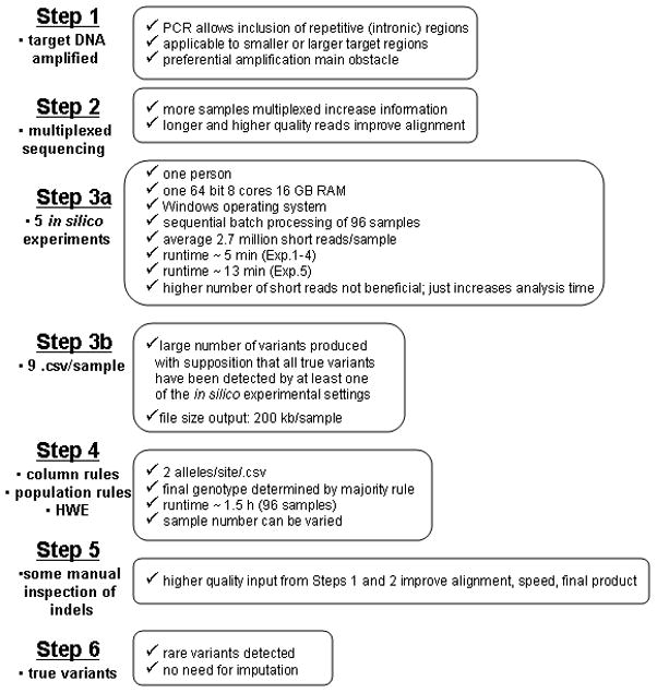
After steps 1 and 2; (Fig. 1) each individual’s reads generated on the Illumina GA and GAIIx were converted to FASTA and run through the five in silico experiments using NextGENe software. Nine output files were produced by the software for each individual because we separated the paired ends for the first four experimental settings and placed the paired ends together for the fifth. Each output file (.csv) consisted of a column listing all sites within the input reference identified as a putative variant for each specific parameter setting. The columns from the nine output files were then merged, ordered from left to right, and aligned horizontally, according to the site index number. The merging of the nine columns per individual resulted in recognizable 2-D patterns (Supplementary Fig. 1). The next step was to discriminate the TP from FP 2-D patterns (Supplementary Fig. 2).

Figure 1. General Workflow.

2.5. Classification of patterns and column rules

Because we wanted to analyze a group of individuals all at one time, we had to contend with the inherent variability encountered with a real vs. simulated dataset as well as the variability of 96 samples vs. 1 sample. We hypothesized if the constant variable; (the five parameters) were applied to each individuals reads, two sets of patterns would emerge differentiating TP from false and ambiguous ones. If all parameters called a variant, a 2-D pattern from the sequential merging of all nine columns would result. The identical variant locations would indicate adequate coverage and unambiguous alignments. On the other hand, if only some parameters detected a variant, it would indicate difficulty in the alignment or a lack of quality reads, and low coverage. Since the paired ends were run separately for experiments 1–4, a setting may not have detected a variant at a site because sequencing did not reach through the insert. All of these issues would manifest themselves as distinct 2-D patterns.

To verify this hypothesis we had prior data verified by the Sanger method from 9.6 kb of non-contiguous sequence of the genomic region under study for all 96 samples. This data served as our training set. The most frequent pattern (75%) for a TP was pattern 1T (Fig. 2), where all parameter settings detected the variant. Interestingly, the second most frequent pattern (9%) for a TP was pattern 3T where experiment 5 alone did not call the variant. Experiment 5 had the paired ends run together and much higher raw read count; thus intimating that a higher number of raw reads does not necessarily correlate with better alignments and more accurate variant calls. Overall there were 16 TP patterns and 12 FP patterns from our training set. The FP patterns were of interest because they consistently displayed perfect classification (i.e. a variant predicted by the software to be true, but which was actually false, displayed one of the 12 patterns). The TP patterns, on the other hand, were variable and the number of them expanded and contracted depending on the quality of the input reads. We therefore designated the FP patterns the “column rules” and removed from our merged dataset of variants any rows which contained one of the FP patterns. This served as an initial elimination of FP.

Figure 2. Categorization of patterns.

The patterns fell into two main groups. Group 1 patterns were those found for true variants. Only five patterns (1T-5T), where “T” stands for true, are shown here. Group 2 patterns were those found for false variants. Only five patterns (1F-5F), where “F” stands for false, are shown here. There were some patterns shared by both groups. This is represented by the shaded oval. Beneath the pattern discovery is an example of one sample where four variants were detected. The variants were detected at sites 3660, 4623, 5220 and 114409. These numbers represent chromosomal locations within the reference sequence of the genomic region of interest. Site 3660 is representative of pattern 1T and site 114409 is representative of pattern 2T. These patterns were found in group1 and were therefore retained. Sites 4623 and 5220 are representative of patterns 1F and 5F, respectively. They were found in group 2 and therefore eliminated. The final output for this sample shows true variants at chromosomal locations 3660 and 114409.

2.6. Population rules preserve genotype accuracy and enable identification of rare variants

After the “column rules” were applied to each individual’s datasets, all datasets across the population were combined for each potential polymorphic locus. This resulted in output files of 96 rows (96 samples), 9 columns each; one for each of the called SNPs/indels. For each of the polymorphic loci, the number of samples which had the variant (n) was calculated; for instance, was the variant a singleton (called in one sample), or was it found in two, three or more samples? For each of the loci and for each sample which carried the SNP/indel, the number of parameter settings which did not call the variant (i.e. failed) was calculated. A potential SNP/indel was then excluded from the final list of variants if too many experiments failed. These filters, designated the “population rules” was designed to assure genotype accuracy across the population; a vital prerequisite for subsequent clinical and research usage. High percentages of failed experiments were indicative of systematic alignment difficulties within a region, which would compromise correct zygosity determinations per sample. Our acceptable percentages of failed experiments were determined by a Sanger verified subset where (Supplementary Figs. 3 and 4c) a SNP was considered a FP if the total failed experiments (TFE) ≥ 9n(.25) [n = 1 or 2]; TFE ≥ 9n(.30) [n = 3]; TFE ≥ 9n(.31) [n = 4–96] and an indel was considered a FP if TFE ≥ 9n(.50). Correct indels were detected with more failed experiments because of their inherent alignment difficulties. The application of the “population rules” also enabled the identification of singletons since sequence data from one individual does not allow for the distinction between common or rare variants.

2.7. Cross-validation and overall classifier performance

To validate whether we could correctly classify TP from FP, we tested and validated three additional test sets whose classes were unknown to the algorithm. The first test set consisted of the same 96 CA samples, but over 66 randomly selected unique sites per individual; none of which overlapped with the initial 9.6 kb. These sites were in introns, 3′UTR and 3′FR. The second test set consisted of 43 tumor samples over 9.6 kb per individual, totaling 412,800 loci from which to assess false positives and false negatives. The third test set consisted of 4 anonymous pooled samples over 5.5 kb per individual, totaling 22,000 loci from which to assess false positives and false negatives. The 5.5 kb region was on chromosome 4. In all three test sets, the same patterns emerged. We quantified the sensitivity TP/(TP+FN), specificity TN/(TN+FP) and (PPV) positive predictive value TP/(TP+FP) of our multi parameter algorithm. Our results showed a sensitivity of 97.8%, specificity of 98.4% and a PPV of 98%. These results reflect almost perfect classification between true and false variants.

2.8. Additional downstream filters required for accurate automated indel detection

Indels and SNPs called by the NextGENe software for each of the five-parameter settings were separated into two bins. Deletions were further categorized into three types: (1) Simple (multi) deletions were defined as a ≥ 2 bp deletion of the same nucleotide (CGTTTTTTACTG). (2) Single (non-multi) deletions were defined as a 1 bp deletion (ATCGTCAAT) or (TGCCCCCCCTACG). (3) Complex (multi) deletions were defined as unique, non repetitive, nucleotide sequences of any size, which consistently appeared as a unit in each experiment (Supplementary Table 3) (CAGTGAGCCGAGAT) (Fig. 3). Output files from the software showing ≥ 10 consecutive deletions of the same nucleotide were considered unreliable and consequently removed. On the other hand, < 10 predicted consecutive deletions of the same nucleotide were retained and probed by our “poly-X” program. The “poly-X” program calculated the lengths and locations of homopolymers within our 160 kb target region. In the examples above, the simple (multi) sequence shows a 2 bp deletion within a homopolymer tract of six T’s and the single (non-multi) shows a 1 bp deletion within a homopolymer tract of seven C’s. Both would be retained for further inspection. The 2 bp deletion (TT) would be designated true if the fraction of reads corresponding to the reference allele had frequencies ≤ 2% of each other [Ref allele = T (75%); Alternate allele = Del (25%) and Ref allele = T (74%); Alternate allele = Del (26%)]. If both were deleted, they should be appearing as a unit since both are on the reference allele. Complex (multi) deletions also appeared as units and this concept took precedence over frequency. For example if the fraction of reads corresponding to all nine reference nucleotides TGAGCCGAG had allele frequencies ≤ 2% of each other for experiments 1 and 2, it was retained as a 9 bp deletion for those parameters. If the reference nucleotides TGAG (Supplementary Table 3) each had read allele frequencies of 52.17%, CCCG each had frequencies of 60%, A had a frequency of 42.11% and G had a frequency of 41.38% for experiment 3, all nine bp were retained even though they did not meet the 2% criteria. This is because beginnings and ends of reads vary within the alignment, and the chances of observing inconsistent frequencies increased with larger units. The fact that the 9 bp unit appeared together consistently across multiple parameter settings took precedence over the percentage requirement. We verified both the homozygous and heterozygous forms of this deletion with Sanger sequencing (Fig. 3). After the application of the “column” and “population” rules, the remaining putative indels were manually inspected. It should be mentioned that because larger HPs (>11 bp) were concentrated in two genomic regions: chr6:35,764,693–35,796,082 and chr6:35,718,599–35,764,558, this method loses indel data in these two areas only.

Figure 3. 9bp deletion (a–c).

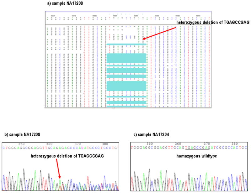
a) NextGENe output of heterozygote deletion of TGAGCCGAG for sample NA17208. This was our largest complex indel. b) Sanger chromatogram of the same deletion for sample NA17208. c) Sample NA17204 did not show a deletion at this site as verified by Sanger chromatogram.

2.9. Indels and SNPs discovered

Overall, a total of 57,929 SNPs and 17,258 indels were detected over the 160 kb region by the five in silico experimental settings for all 96 individuals. The assumption was that all true variants had been identified by at least one of the in silico experimental settings and the remainder were false variants. By applying our selective filters, we were able to reduce the number to 613 SNPs and 57 indels (Supplementary Table 4). Of the 57 indels 16 were insertions, 41 were deletions, 21 were singletons and 35 had frequencies over 1%. 34 of the indels were within genomic regions of repetitive elements and 22 were within or immediately next to a homopolymer. Our largest complex microdeletion was 9 bp in length and our largest structural variant was 3.3 kb in size. Both of these were verified with Sanger (Fig. 3a–c). Of the SNPs, 313 were singletons and 300 were common polymorphisms.

2.10. Subtle changes in parameter settings produce different results

For the first four in silico experiments, the initial read length of 49 bp increased on average to 66 bp after consolidation, and the percent of alignable reads decreased from 94% to 84%. Interestingly the correlation between read count and percent of alignable reads were not as expected; for example NA17222 with a lower read count had 95% alignable reads before consolidation and 91% after. NA17290, with a higher read count had 95% alignable reads before consolidation and 74% after, thus intimating that although original read count is important and a certain minimum threshold is necessary, the quality of those reads, as well as the insert size [26], is of equivalent importance. The percent alignable reads diminished on average from 68% to 44% after elongation for experiment 5. When comparing the five in silico experiments for numbers of called variants, parameter 4 produced the largest number (1113 calls) and parameter 3 the lowest (97 calls). The sensitivity and specificity of individual parameters was also assessed before application of the PR methodology. While parameter 1 displayed the highest sensitivity (90%)-meaning 90% of the called variants were correctly classified as true, it also showed 65% specificity - an indicator of too many FP. Parameter 3 displayed the highest specificity (86%). Parameter 5 introduced reads with sequencing errors into the alignment, resulting in numerous tri-allelic calls and consequent FP. After application of our PR methodology, a significant improvement was observed with both specificity and sensitivity increased to 98%.

2.11. Variability in coverage can be biological or due to technical issues

Sequence coverage depth is highly variable with NGS technology. For one individual, the number of reads mapped to a base within the reference can fluctuate dramatically from <1x to ≫200x, dependent on variables such as the number of raw reads, quality and length of the reads, complexity of the genomic region, sequencing technology used, preparation techniques and human error. This variability is amplified when analyzing 96 unique individuals simultaneously (Fig. 4). We defined read depth as the number of times a base within the reference in the region of interest, was covered by a mapped read. We defined coverage as the number of bases within the target region which were covered by reads. Experiments 1–4 showed the effects of “consolidation”, where the number of reads was reduced and the coverage was more uniform. The mean read depth was 52x and the mode 56. Many polymorphic sites were detected below 20x read depth with the lowest in a single sample after consolidation at 4x. Experiment 5 had the paired ends run together and the raw read count maintained resulting in a much higher mean read depth of 1533x. FP however were still found, which was consistent with previous reports [23].

Figure 4. Variability of Coverage.

Variants were discovered at variable read depths. The x-axis shows the location of each variant discovered, from 5′(left) to 3′(right). The y-axis is the average read depth across all 96 individuals. SNPs at the highest read depth, (above 100x) and the lowest (below 20x) are circled.

Since the quality of DNA, the library preparations, and the number of raw reads were inconsistent for each individual, “gaps” or zero coverage locations were also highly variable. To study this, we produced a so-called population reliability index based on experiment 5 (Supplementary Table 2). The population reliability index ascertained the number of gaps per individual. Experiment 5, unlike the other experiments maintained the original read counts and therefore assured us the gaps were not caused by lower read depth because of consolidation of the reads. Gaps ≥ 100 bp were designated “major” and any gaps < 100 bp were designated “minor”. Major/minor values were assigned to each of the 96 Caucasians. For instance NA17292 had values of 21/120, showing that this subject, in experiment 5, had 21 coverage gaps of size ≥ 100 bp and 120 smaller gaps < 100 bp. Overall, NA17292 had an average coverage of 95.3% across the entire gene. Since the major/minor and average coverage values did not represent the precise chromosomal locations where zero or low coverage areas were occurring, a visual representation was made of the reliability index called the “gap map” (Supplementary Fig. 5). When viewing the population gap map, it is easy to see where there are consistent coverage problems that most likely are due to technical issues, or could be biological, such as structural variation. Eight of these areas are bracketed (Supplementary Table 5), and when inspected, contain repetitive elements. The chromosomal region also shows possible structural variation and two areas particularly stand out as being consistent across the samples; regions 4 and 5. At first it was thought these gaps were true deletions, but region 4 had already been successfully sequenced using Sanger technology on all of our samples, and no sample showed a deletion. Region 5 was the largest gap and was also perceived to possibly be a deleted area. We therefore sequenced, using Sanger technology, through the area on some of our samples, and the results showed a 3.3 kb deletion.

2.12. Verification of results with other methods

Several measures were taken to validate results. The Sanger method of sequencing, long considered the “gold standard” for accuracy, was used for the establishment of, and to verify our NGS training set. Overall, 922 kb were interrogated for FP and TP. Our results showed all positions in the population correctly identified with the exception of “gap 4”, where there was zero coverage, and 5 sites which were discordant (Supplementary Fig. 5). This resulted in a 99% concordance of genotypes between Sanger and NGS.

For verification of the first test set, each of the 96 samples were genotyped using the Illumina 550Kv3 and 510S SNP chips, as well as Affymetrix 6.0. Of the 5071 genotypes, 81 were discordant between Illumina/Affymetrix and NGS, resulting in 98.4% concordance. It should be mentioned that two of the SNPs, one from Illumina (rs7749607:C>T) and one from Affymetrix (rs9470065:G>A) we did not find in any of our samples with NGS. To validate this further, we used Sanger sequencing and found the NGS results in agreement for rs9470065 but not for rs7749607. The single sample in which rs7749607 was found had a reliability index of 3/31, indicating numerous gaps and consequent alignment ambiguities (Supplementary Table 2).

Two additional sample test sets were verified with Sanger sequencing. The first consisted of 43 anonymized tumor samples over the same 160 kb region on chromosome 6. 9.6 kb for each sample was verified. All polymorphic and monomorphic sites were correctly identified except where there was zero coverage in one of the CpG islands and two sites where the Sanger results were inconclusive and therefore a comparison could not be made. The second set consisted of 4 anonymized and pooled DNA samples over a 5.5 kb region on chromosome 4. All variant sites were detected with no missed sites. Additional regions, totaling 1 kb were sequenced to verify indels.

On a broader scale, heterozygosity, (π) was calculated for the entire 160 kb region, as well as regions within the gene structure (Table 2). These values were striking, showing a 40-fold difference (π = 0.00002 – 0.0008) between flanking regions, introns and UTRs, intimating unique genetic histories at these loci. Higher heterozygosity in GC-rich areas agreed with previous reports of similar findings [27].

Table 2.

Nucleotide Diversity.

Region	Tajima’s D	Heterozygosity (π) ± SE	Length (bp)	GC Content	AT Content	Number of SNPs Within Each Region	Number of Singletons in this Region
5′FR	0.512	0.0008 ± 0.0006	1045	59%	41%	4	2
5′UTR according to mRNA BC042605.1	−0.96	0.00003 ± 0.00003	297	60%	40%	2	1
Intron 1A	−0.58	0.0006 ± 0.0003	7959	52%	48%	40	16
Intron 2A	−0.28	0.0006 ± 0.0003	31390	46%	54%	133	63
5′UTR according to mRNA NM_004117.2	ND	ND	153	73%	27%	0	0
Coding region	−1.09	0.00005 ± 0.0001	1374	45%	55%	2	1
Intron 1	−1.44	0.0003 ± 0.0001	45960	39%	61%	159	82
Intron 2	−1.37	0.0004 ± 0.0002	5561	39%	61%	27	13
Intron 3	−1.87	0.0002 ± 0.0001	16739	40%	60%	70	33
Intron 4	−1.29	0.00002 ± 0.00009	921	37%	63%	2	2
Intron 5	−1.81	0.0003 ± 0.0001	21691	40%	60%	97	50
Intron 6	−1.85	0.0002 ± 0.0001	6027	41%	59%	27	17
Intron 7	−1.65	0.0001 ± 0.0001	4012	43%	57%	13	8
Intron 8	−2.25	0.0002 ± 0.0001	6812	41%	59%	39	25
Intron 9	−2.04	0.00008 ± 0.0001	2802	39%	61%	10	7
Intron 10	−1.44	0.0001 ± 0.0002	1051	48%	52%	4	2
3′UTR	−1.64	0.0003 ± 0.0003	2245	40%	60%	14	10
3′FR	−0.13	0.0006 ± 0.0005	938	42%	58%	4	2

N.D. stands for “not-determined” Loci which did not conform to HWE were not included in the calculations.

As another form of validation, we looked at dbSNP130. 258 of the SNPs/Indels we found were also in dbSNP, although the genotypes for our 96 CA individuals, utilizing this database, were not available to compare. In several cases, the dbSNP variant, although at the same chromosomal location, did not agree with ours. For instance; at rs35311317 dbSNP has a C>T SNP while NGS found a C insertion. We validated this and the Sanger results agreed with our methodology results (Supplementary Fig. 6 a–c).

Our final means of validation was assessing whether our genotypes conformed to Hardy-Weinberg equilibrium (HWE) expectations. Deviations from HWE can be due to inbreeding or population stratification, but also can be due to problems with genotyping [28]. Using (P > 0.001), 22 loci were found to be out of HWE and none of them were in linkage disequilibrium with each other [29, 30], indicating that the reason they deviated from HWE most likely was due to genotyping errors among one or more samples. Of the 22 loci, 10 were discovered to be within areas of poor coverage and adjacent to large gaps in sequencing. The remaining 12 were indels, indicating our zygosity threshold determinations for indels may not be optimal.

2.13. Comparison with HapMap and 1000 Genomes Project Data

Realizing the genetic variation in the CEU samples may not be identical to that found in ours, and that the sample sizes are different, we set out to see if the common polymorphisms detected by our method for this genomic region on chromosome 6 were also present in the HapMap and the 1000 genomes (1KG) project data deposited in dbSNP130. All the HapMap CEU common polymorphic sites were in agreement with our findings with the exception of (rs3734257:G>A) which in the CEU population had a 1.7% frequency in 120 alleles and was monomorphic in our 192 alleles.

168 common polymorphisms, of which 36% are supported by other platforms such as dbSNP, Sanger, Illumina and Affymetrix, were detected by our method. These were not found in the low or deep coverage 1KG pilots as noted in dbSNP130. 83 of these markers had frequencies greater than 3%. Furthermore, two large gap areas, one of which we had prior Sanger data on, contained high frequency SNPs. These correspond to gaps 4 and 5 on the reliability gap map. Gap 4 is a GC-rich area and our method was able to detect 3 out of the 3 high frequency SNPs within this region; (rs9462103:C>T), (rs13215797:C>T) and (rs10947564:T>C), although because of very low coverage across the entire population and therefore unreliable genotypes we excluded all three from our final data set. 1KG detected rs13215797 alone. Gap 5 contained an Alu and although we were able to verify a 3.3 kb deletion in some of our samples using Sanger, 1KG also did not detect anything in this area.

2.14. Methodology outperforms existing software

MAQ (http://maq.sourceforge.net/) is an open source and easy-to-use software which has been used extensively for variation discovery [31–34]. It maps short reads and calls genotypes. We ran MAQ, version 0.7.1 on 20 of our 96 samples over the 120 kb region on chr6: 35,768,636–35,648,407. Using the default parameters, the SNP filter and loading both paired ends, we compared the SNP and indel calls from MAQ to our results. Overall MAQ detected a total of 435 SNPs and 13953 indels in our 20 samples. Our method identified a total of 292 SNPs and 24 indels. A variant was considered validated if it was seen in our Sanger traces, Illumina/Affymetrix data or dbSNP. From our set of 887 validated sites, we were able to compare the number of FP and FN between the two methods. Our method showed 0% FP for both SNPs and indels. MAQ showed 9% FP for SNPs, with only 1.1% of the indels verified as true. As for false negatives, our method showed 0.75% and 0.13% for SNPs and indels, respectively. MAQ showed 11% FN for SNPs and 0.26% for indels. To further evaluate our method, we compared our SNP and indel calls on the same 20 samples, and over the same 120 kb region with SAMtools, version 0.1.16 [35], and GATK, version 1.1–10 [36], respectively. Using BWA, version 0.5.9 as the aligner and the “mpileup”, “varfilter” and “Unified Genotyper” tools, we obtained FP and FN. Our results, using SAMtools, showed 7% FP and 55% FN for SNPs. GATK showed 18% FP and 7% FN for indels. The high FN rate is likely due to this software’s very stringent default parameters for calling a SNP or indel.

2.15. SNP in hormone response element in LD with silent (synonymous) SNP

Our method identified a SNP (rs73746499:T>C) at a critical position within a HRE [8, 18]. We found rs73746499 to be at relatively high frequency in our study, with 3.1% of our 96 Caucasian subjects carrying the variant. Further inspection showed 22 additional SNPs and one 5 bp deletion in LD (r²=1) with rs73746499 (Fig. 5, Supplementary Table 6). 22 of the variants were in introns, one was a synonymous SNP in Exon 10 (rs34866878:C>T), and one was in the 3′UTR (rs41270080:G>T). Eleven of these variants discovered by our method, including the deletion, were novel and not reported elsewhere. The LD between them had also not been discovered or examined.

Figure 5. Variants in LD.

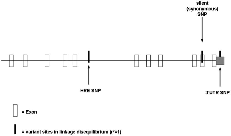
Schematic diagram illustrating FKBP5 genomic organization (NM_004117.2) and the location of 3 of the 24 variants in linkage disequilibrium (r²=1).

Since the Exon10 and 3′UTR variants were part of the mRNA and both synonymous SNPs and 3′UTR variants have been shown to have functional consequences such as inducing structural changes which could affect protein binding [37–40], drug interactions or alter mRNA stability, we used Mfold 3.1 [41] to predict the secondary structures for the full-length wild-type, Exon 10, 3′UTR, and (Exon 10-3′UTR) haplotype mRNA transcripts. The Exon 10 synonymous SNP showed a change in calculated free energy and secondary structure, whereas the wild-type, 3′UTR and (Exon 10-3′UTR) haplotype SNPs showed no changes (Fig. 6).

Figure 6. Effects of silent and 3′UTR SNPs on predicted mRNA secondary structures (a–h).

a through h are the mRNA folding structures predicted by Mfold. a) and b) are the wild-type structure with snapshots of the Exon 10 (a) and 3′UTR (b) local stem-loop structures; ΔG =−995.33 kcal/mol. c) and d) are the Exon 10 variant (c) and 3′UTR wild-type (d) structures; ΔG =−986.64 kcal/mol. The c and d haplotype codes for the least stable structure. e) and f) are the Exon 10 wild-type (e) and 3′UTR variant (f) structures; Δ G =−995.22 kcal/mol. g) and h) are the Exon 10 variant (g) and 3′UTR variant (h) structures; Δ G = −991.97 kcal/mol. The boxes in the left-hand corners of c, e and g are from SNPfold and represent the c–d, e–f, and g–h haplotypes. The x-axis is the nucleotide position of the mRNA and the y-axis is the average change in partition function. This is determining the extent to which the wild-type and SNP matrices differ, as well as where the base-pairing probabilities are most different.

Since RNAs generally adopt multiple conformations, we used SNPfold [42] to determine whether our SNPs had a large effect on the RNAs structural ensemble. SNPfold computes all the possible suboptimal conformations of the RNA strand and determines the probability of base-pairing for each nucleotide. By evaluating all possible mRNA structures, we predicted if the SNPs had an affect on the probability of base-pairing (accessibility) of critical interaction sites on the mRNA when compared to the wild-type. According to SNPfold, the Exon 10, 3′UTR, and haplotype (Exon 10-3′UTR) variants significantly disrupted the RNA structural ensemble in specific regions of the mRNA (Figs. 6 and 7). Notably, the Exon 10 variant, which is part of TPR3, also disturbed an adjacent region corresponding to TPR1; an effect not observed with the 3′UTR variant alone. The interaction of immunophilins like FKBP5 with hsp90 occurs through the TPR domain and is conserved in plants as well as the animal kingdom [43]. We found this area conserved, and not polymorphic, with the exception of the single synonymous SNP in Exon 10.

Figure 7. The “silent” SNP affects base-pairing probabilities within TPR domains.

SNPfold graph is a zoomed-in view of the “silent” SNP (green vertical line) and its affects on the mRNA. Nucleotides 960–1059 of the mRNA correspond to TPR1 when translated (first pink shaded area). Second pink shaded area corresponds to TPR2 when translated. Third pink shaded area corresponds to TPR3 when translated. Note the absence of perturbations within TPR2 and areas preceding the TPR domain.

2.16. Variants in RBP and RNP binding sites may affect posttranscriptional gene regulation

Because RNA-binding proteins (RBPs) and ribonucleoprotein complexes (RNPs) partly control gene expression by regulating RNA transcript translation and stability, we used data obtained by the PAR-CLIP (Photoactivable-Ribonucleoside-Enhanced Crosslinking and Immunoprecipitation) [44] method to explore whether the FKBP5 mRNA was bound by RBPs and RNPs. Data showed Argonaute (AGO) and trinucleotide repeat-containing (TNRC6) proteins, both part of the miRNA induced silencing complexes [45], binding to segments of RNA within the 3′UTR of FKBP5. AGO and miR-124, one of the most conserved and abundantly expressed miRNAs in the adult brain [46], were bound to the same site in Exon 9. Insulin-like growth factor 2 mRNA-binding proteins (IGF2BFs) was the most abundant RBP, binding to sites predominantly in the 3′UTR. Our methodology uncovered genetic variants within seven of these binding sites; 5 of which were novel (Supplementary Table 7a–b).

2.17. Discovery of rare variants impacts evolutionary conclusions

Our method detected 267 novel rare variants (<1%) within the chromosomal region encompassing FKBP5. The negative Tajima’s D value of −1.44 conflicted with previous reports of this region on chromosome 6 as being under balancing selection and upon inspection, the dissimilar reports were based on small datasets which disregarded low frequency variants [47, 48]. Our complete NGS data showed a dramatic increase in low frequency polymorphisms, thus changing the landscape of evolutionary conclusions.

3. DISCUSSION

Current methods for the analysis of next-generation sequencing data mostly involve a one-size-fits-all solution, where either default settings or one set of parameters are used. This would be adequate if there was no variability in the DNA quality, LR-PCR primer design and conditions, fragmentation, library preparation, cluster differentiation determination, insert size and platform used. All these factors contribute to the integrity of the reads which eventually are assembled and aligned to the reference. A one-size-fits-all strategy can lead to incorrect genotypes and the detection of false variants as well as missed de novo variants.

Our method, using pattern recognition 1) reduced the number of false variants resulting in near perfect classification between true and false positives 2) detected 313 singletons, 267 of which were novel, 3) detected variants in variable read depth coverage regions ranging from 4x to over 100x, 4) determined genotypes with 99% concordance with other platforms, 5) detected 57 indels, 36 of which were novel, 6) analyzed multiple individuals simultaneously which allowed us to calculate LD without the need for imputation 7) was amenable to automation, which is a prerequisite for clinical usage and 8) was amenable to individual labs without the need for extra personnel or resources.

While this study represents a novel approach to analysis, it also serves as an example of the biological insights that can be gained by a comprehensive dataset as exemplified by our method using PR. The level of detail and accuracy we achieved could not have been obtained using current methods for analysis of high-throughput data, by using imputation, or by selecting SNPs from databases such as dbSNP, HapMap or 1KG where rare variants, indels and variants in non-coding regions are severely underrepresented and restricted to the available populations.

Our method enabled the discovery of genetic variants within FKBP5 mRNA binding sites. SNPs can alter mRNA secondary structure and expose regions of RNA to binding of proteins, which could inhibit translation, thereby affecting individual posttranscriptional gene regulation. Although the PAR-CLIP siRNA knockdown experiments designed to assess whether IGF2BP proteins stabilized their target mRNAs were not performed on FKBP5, the clustered selective binding of IGF2BP to the 3′UTR of FKBP5 mRNA suggests it may be regulating the gene. IGF2BP has been associated clinically with altered glucose levels [49].

Our method enabled the discovery of an intronic SNP within a HRE. The HRE SNP was in perfect LD with 22 noncoding variants, and one coding SNP. Because conservation of LD may be a marker of functionally important allelic combinations [50], and evidence of selection, we aligned the nucleotide sequences of 9 mammals, including 4 non-human primates. Both the Exon 10 and 3′UTR loci showed the same consensus nucleotides as the human wild-type. Two exceptions were the mouse and guinea-pig (hystricomorph rodent), which showed the human variant at both loci (Supplementary Table 8). Interestingly both the Exon 10 and 3′UTR loci, across 9 mammals, had the same consensus nucleotides (when the wild-type nucleotide was present in Exon 10, it was also present in the 3′UTR; when the variant nucleotide was present in Exon 10, it was also present in the 3′UTR), implying some association between the two loci.

In addition, when examining the partition function for the Exon 10 SNP, it predicted that the variant perturbs more than one of the 3 unit repeats within the TPR domain of FKBP5. This suggests the synonymous Exon 10 SNP may be affecting a critical region necessary for function. Differences in conformation at sites where drugs and modulators interact may appear subtle at the molecular level, but can produce significant biological results [51]. Since RNA interactions are identified by both computational and biochemical approaches, and similar results were obtained using two different algorithms (Mfold and SNPfold); biochemical assays (in vitro or in vivo) will be needed to determine the phenotype of this haplotype and which of the 24 variants, if any, is dominant in exerting an effect.

A comprehensive dataset, as achieved by our methodology, could enable the identification of rare disease causing variants. It could also change the way future assays are designed. The microscopic view, where a single variant is investigated in isolation could be replaced by a more global view, where variants are investigated in the context of their genetic environment, for their interactions with each other and for their combined impact on function and influence on disease risk. The use of LD as a purely statistical tool in imputation and GWAS could evolve into the investigation of the biological effects of LD and the examination of the underlying reasons behind it; one of which is selection. This has special significance since complex diseases are most likely influenced by the interactions of multiple loci. Our findings may be clinically relevant. We report for the first time, a synonymous SNP within FKBP5 which is predicted to alter mRNA stability, to be in perfect LD with a regulatory region determined to impact GR sensitivity and bioavailability. Since FKBP5 serves as a modulator of steroid receptor function, and the expression of the gene is a key determinant in that regard, we hypothesize our findings may in part explain regulation through interactions with hsp90, or by impacting protein translation efficiency. For example, synonymous SNPs, such as in the P-glycoprotein, have been shown to alter the translation kinetics of mRNA and produce a conformationally changed protein [52]. It should also be noted we did not find any carriers of the homozygous variant in our population. In addition, there are reported ethnic differences between CA and African Americans (AA) regarding their sensitivity to glucocorticoids [53]. Interestingly, in a study of 96 AA (unpublished data), the AA had a significantly higher Exon 10 variant allele frequency (20%) than CA (3%), and carried the homozygous variant.

3.1. Improvements and limitations

There are a number of potential improvements and limitations to our methodology in its present state. Our study focused on a 160 kb targeted region. The overall PR concept could be adapted to a whole genome, but faster aligners which use Burrows-Wheeler transform (BWT) would need to be evaluated for their performance, since alignment was a crucial feature in our design.

Our detection of indels involved some manual inspection for verification. Although we did not automate this part for the present study, it could be done. Our detection of indel loci was accurate, with 47% of our indels verified, but the percentage cut-offs for zygosity determination, whether heterozygous or homozygous, were not optimal and need to be improved. Unlike most methods, which designate lower and upper allele frequency boundaries, we omitted a lower boundary for the nucleotide(s) that are deleted or inserted. Our upper boundary for simple (multi) and single (non-multi) deletions and insertions is <80% for heterozygotes and ≥ 80% for homozygotes. More samples with indels need to be tested for further optimization.

We were able to analyze 96 individuals over a 160 kb region in only 1.5 hours and with one computer. Our output included chromosomal locations, frequencies, genotypes, HWE calculations and RefSNP ID from dbSNP. If adding the run-time for the 5 experimental settings using NextGENe’s batch processing option, it would take ~2 days to complete 96 individuals. This is significantly faster and less expensive than using methods which require additional verification [25]. The total run-time could even be reduced to 2 hours if the experiments were run in parallel rather than sequentially on one computer.

Two major technical issues in this study which caused a loss of information and inaccurate results, were the presence of “gaps” or no coverage regions and preferential allelic imbalance; both issues of DNA quality, PCR and sequencing. While shorter and overlapping LR-PCR amplicons as well as careful PCR primer design can offset the allelic imbalance, the gaps were puzzling and seemed to consistently occur in repetitive regions. To investigate possible causes, we increased the number of raw reads, reasoning that a higher read count may reduce the number of gaps and increase coverage, but in some cases, the exact opposite occurred. It should be noted that we were able to achieve saturation levels of reads per individual whether multiplexing or loading a single sample on a flow cell (unpublished observations). We did not find a higher read count correlating with more uniform and complete coverage across the region of interest. This reinforces the principle that coverage is associated with both quality of reads and sequence context rather than just raw read count. Therefore the high cost which is often cited as a prerequisite for high read counts and consequent greater coverage may be avoidable.

4. CONCLUSION

Our PR method is novel in that it introduces for the first time an alternative way to detect SNPs and indels from high-throughput data. Other methods use a “top-down” approach, which produce either too many FP or too many FN, depending on the threshold values chosen. The thresholds, which are unavoidable when using software, provide an “either/or” solution, and the final outcome is dictated by those choices (parameter settings) [54]. The genetic variants detected by other methods are a result of one set of conditions. With one set of conditions it is impossible to select the right combinations to accommodate the many unknowns (input read quality), complexities (genomic sequence) and variables (sample preparations and human error) encountered and expect to achieve a precise and accurate set of variants. In contrast, the genetic variants obtained by our method result from multiple sets of parameters which are designed to mimic “real world” unknowns and inconsistencies; unknowns which most likely will always be present in DNA, because of its inherent repetitiveness and ambiguity, and sample preparation techniques.

With longer and more accurate reads as well as improved target enrichment methods [55–57], we believe the data input will become of higher quality and sequencing through repetitive regions, thereby eliminating gaps, will be solved. Therefore this method of analysis will produce consistent, fast and reliable results for research and clinical purposes [58]. It is our hope that the general pattern recognition concept presented here represents one small step towards bridging the gap between sequencing and analysis [59] and the dataset in this study provides information for future research.

5. MATERIALS AND METHODS

5.1. Human DNA samples

DNA samples from 96 Caucasian-Americans were obtained from the Coriell Cell Repository (Camden, NJ), Human Variation Panel – Caucasian Panel of 100 (www.coriell.org/). In addition, 43 tumor samples and 4 anonymized clinical samples were used. Written and informed consent was obtained from all subjects on their use. Our studies were reviewed and approved by the Mayo Clinic Institutional Review Board.

5.2. Public databases and software

The human reference genome was obtained from NCBI, Build 36 v3. NT_007592.14; subsequence 26,398,617–26,558,272 and NT_016354.19; subsequence 89,146,844–89,218,953. The cDNA reference sequences were NM_004117.2, NM_004117.3, BC042605.1 and NM_000297.2. HapMap data for the CEPH (Utah residents with ancestry from northern and western Europe) was downloaded from http://hapmap.org. The 1000 Genomes project data was obtained from http://browser.1000genomes.org/, and dbSNP Build 130. Software used for analysis was NextGENe v1.04 and 1.10 (SoftGenetics, LLC, State College, PA).

5.3. Short-range PCR for Sanger sequencing

Eleven amplicons, totaling 9.6 kb which targeted 1 kb of the 5′FR, all exons and 152 bp of the 3′UTR of the FKBP5 gene were produced in each of the 96 Caucasian Coriell samples and 43 tumor samples. Four additional amplicons which targeted 1 kb of intronic regions were also produced in the Coriell samples. Each of the 15 reactions was performed in 20 μl containing 10~15 ng genomic DNA, 5 pmol each of forward and reverse primers (Supplementary Table 1) and FastStart Taq DNA polymerase (Roche, Indianapolis, IN). PCR cycling parameters included 95ºC for 5 min, 30 cycles at 95ºC for 30 s, 55~59ºC for 30 s, 72ºC for 30~120 s, and a final extension at 72ºC for 7 min. PCR products were subsequently purified with ExoSAP-IT (USB Corporation, Cleveland, OH). Amplicons were sequenced on both strands with an ABI 3730 DNA sequencer using ABI BigDye Terminator sequencing chemistry. All chromatograms were analyzed using Mutation Surveyor v 2.2 (SoftGenetics, LLC, State College, PA). Both the forward and reverse strands were manually inspected. The PCR primers and conditions for the 4 anonymized clinical samples were as previously described [60].

5.4. Statistical analysis

An exact test was used to test Hardy-Weinberg equilibrium. Linkage disequilibrium was calculated as the D’ and r² measures. π (average difference between nucleotide pairs) and Tajima’s D measures were estimated as in [61]. Agreement of next-generation sequencing and other genotyping techniques was calculated as the number of sites in agreement between the platforms over total number of sites considered. A confidence interval for this agreement measure was constructed using a sandwich estimator assuming compound symmetric covariance, where clusters were individual samples.

5.5. Threshold determinations

When building a model with real and uncertain datasets, it is impossible to accurately define optimal parameter thresholds; therefore logical estimates must be chosen. Using concepts from SA and knowledge of performance metrics of the Illumina platform, we selected thresholds for three features; mutation percentage, coverage and matching base percentage. The mutation percentage remained constant, at 20%, while the coverage included parameter settings with levels >3x and >10x. The coverage values were derived from the 1KG deep coverage trio pilot (pilot 2); with an average coverage of 10x for Solexa/Illumina platform centers, and low coverage (pilot 1); with an average coverage of 3x. The mutation percentage, calculated after duplicates were removed, was set at >20% to remove random and systematic sequencing errors. Both the mutation percentage and coverage thresholds had to be exceeded for a variant to be called real at that position. The matching base percentage minimum and maximum levels were selected so that the probability of an actual value being outside that range was ~10%. The range (50%–92%) was representative of the variability encountered in real-world datasets. Thus, the 50%, less stringent alignment setting in experiments 1 and 2, acted as a “catch-all” threshold, detecting false positives as well as true positives. Concurrently, it served as an eliminator of false negatives.

5.6. Method implementation

The “poly-X” and downstream filter programs are available upon request. A Java program; designated “poly-X”, calculated the chromosomal location(s) and lengths of each homopolymer tract [poly (dA), poly (dT), poly (dG), poly (dC)] within the reference of a specified target region. A HP was defined as a single nucleotide repeat ≥5 bp [62]. Information from the “poly-X” program was then integrated into the detection of deletions. Only simple (multi)and single (non-multi) deletions detected in homopolymer regions ≤ 11 bp were considered putative true variants. A Perl program parsed the nine NextGENe reports produced by the five experiments for each sample, merged them and applied “column-based” rules to filter out false polymorphic sites. A preliminary summary report of the polymorphisms that met the thresholds was produced for each sample. A Java program then collected all of the sample summary reports and applied “population-based” rules to further determine the true polymorphic sites across the population. For a structured flowchart (Nassi-Schneiderman diagram) of the overall algorithm, column and population rules see (Supplementary Fig. 4a–c). The “poly-X” and downstream filter programs required input files in FASTA and .csv, respectively.

Highlights.

• Pattern recognition approach produces higher accuracy than current methods

• We are able to detect rare variants and indels

• We show perturbations in a critical binding site of FKBP5 mRNA

• We provide possible explanation for individual differences in GR sensitivity

Appendix A. Supplementary data

Supplementary data associated with this article can be found, in the online version at doi:…………………..

References

- 1.Chakravarti A. Population genetics--making sense out of sequence. Nat Genet. 1999;21:56–60. doi: 10.1038/4482. [DOI] [PubMed] [Google Scholar]
- 2.Sabeti PC, Schaffner SF, Fry B, Lohmueller J, Varilly P, Shamovsky O, Palma A, Mikkelsen TS, Altshuler D, Lander ES. Positive natural selection in the human lineage. Science. 2006;312:1614–1620. doi: 10.1126/science.1124309. [DOI] [PubMed] [Google Scholar]
- 3.Lieberman-Aiden E, van Berkum NL, Williams L, Imakaev M, Ragoczy T, Telling A, Amit I, Lajoie BR, Sabo PJ, Dorschner MO, Sandstrom R, Bernstein B, Bender MA, Groudine M, Gnirke A, Stamatoyannopoulos J, Mirny LA, Lander ES, Dekker J. Comprehensive mapping of long-range interactions reveals folding principles of the human genome. Science. 2009;326:289–293. doi: 10.1126/science.1181369. [DOI] [PMC free article] [PubMed] [Google Scholar]
- 4.Marguerat S, Wilhelm BT, Bähler J. Next-generation sequencing: applications beyond genomes. Biochem Soc Trans. 2008;36(Pt5):1091–1096. doi: 10.1042/BST0361091. [DOI] [PMC free article] [PubMed] [Google Scholar]
- 5.Kidd JM, Sampas N, Antonacci F, Graves T, Fulton R, Hayden HS, Alkan C, Malig M, Ventura M, Giannuzzi G, Kallicki J, Anderson P, Tsalenko A, Yamada NA, Tsang P, Kaul R, Wilson RK, Bruhn L, Eichler EE. Characterization of missing human genome sequences and copy-number polymorphic insertions. Nat Methods. 2010;7:365–371. doi: 10.1038/nmeth.1451. [DOI] [PMC free article] [PubMed] [Google Scholar]
- 6.Chen Y, Cicciarelli J, Pravica V, Hutchinson IV. Long-range linkage on chromosome 6p of VEGF, FKBP5, HLA and TNF alleles associated with transplant rejection. Mol Immunol. 2009;47:96–100. doi: 10.1016/j.molimm.2009.01.006. [DOI] [PubMed] [Google Scholar]
- 7.Pratt WB, Toft DO. Steroid receptor interactions with heat shock protein and immunophilin chaperones. Endocr Rev. 1997;18:306–360. doi: 10.1210/edrv.18.3.0303. [DOI] [PubMed] [Google Scholar]
- 8.Hubler TR, Scammell JG. Intronic hormone response elements mediate regulation of FKBP5 by progestins and glucocorticoids. Cell Stress Chaperones. 2004;9:243–252. doi: 10.1379/CSC-32R.1. [DOI] [PMC free article] [PubMed] [Google Scholar]
- 9.Binder EB. The role of FKBP5, a co-chaperone of the glucocorticoid receptor in the pathogenesis and therapy of affective and anxiety disorders. Psychoneuroendocrinology. 2009;34:S186–S195. doi: 10.1016/j.psyneuen.2009.05.021. [DOI] [PubMed] [Google Scholar]
- 10.Bao H, Guo H, Wang J, Zhou R, Lu X, Shi S. MapView: visualization of short reads alignment on a desktop computer. Bioinformatics. 2009;25:1554–1555. doi: 10.1093/bioinformatics/btp255. [DOI] [PubMed] [Google Scholar]
- 11.Bell CJ, Dinwiddie DL, Miller NA, Hateley SL, Ganusova EE, Mudge J, Langley RJ, Zhang L, Lee CC, Schilkey FD, Sheth V, Woodward JE, Peckham HE, Schroth GP, Kim RW, Kingsmore SF. Carrier testing for severe childhood recessive diseases by next-generation sequencing. Sci Translat Med. 2011;3:65ra64. doi: 10.1126/scitranslmed.3001756. [DOI] [PMC free article] [PubMed] [Google Scholar]
- 12.Carver T, Böhme U, Otto TD, Parkhill J, Berriman M. BamView: viewing mapped read alignment data in the context of the reference sequence. Bioinformatics. 2010;26:676–677. doi: 10.1093/bioinformatics/btq010. [DOI] [PMC free article] [PubMed] [Google Scholar]
- 13.Robinson JT, Thorvaldsdóttir H, Winckler W, Guttman M, Lander ES, Getz G, Mesirov JP. Integrative genomics viewer. Nat Biotechnol. 2011;29:24–26. doi: 10.1038/nbt.1754. [DOI] [PMC free article] [PubMed] [Google Scholar]
- 14.Mills RE, Luttig CT, Larkins CE, Beauchamp A, Tsui C, Pittard WS, Devine SE. An initial map of insertion and deletion (INDEL) variation in the human genome. Genome Res. 2006;16:1182–1190. doi: 10.1101/gr.4565806. [DOI] [PMC free article] [PubMed] [Google Scholar]
- 15.Chuzhanova NA, Anassis EJ, Ball EV, Krawczak M, Cooper DN. Meta-analysis of indels causing human genetic disease: mechanisms of mutagenesis and the role of local DNA sequence complexity. Hum Mutat. 2003;21:28–44. doi: 10.1002/humu.10146. [DOI] [PubMed] [Google Scholar]
- 16.Li H, Ruan J, Durbin R. Mapping short DNA sequencing reads and calling variants using mapping quality scores. Genome Res. 2008;18:1851–1858. doi: 10.1101/gr.078212.108. [DOI] [PMC free article] [PubMed] [Google Scholar]
- 17.Mullaney JM, Mills RE, Pittard WS, Devine SE. Small insertions and deletions (INDELs) in human genomes. Human Molecular Genetics. 2010;19:R131–R136. doi: 10.1093/hmg/ddq400. [DOI] [PMC free article] [PubMed] [Google Scholar]
- 18.Paakinaho V, Makkonen H, Jaaskelainen T, Palvimo JJ. Glucocorticoid receptor activates poised FKBP51 locus through long-distance interactions. Mol Endocrinol. 2010;24:511–525. doi: 10.1210/me.2009-0443. [DOI] [PMC free article] [PubMed] [Google Scholar]
- 19.Kent WJ, Sugnet CW, Furey TS, Roskin KM, Pringle TH, Zahler AM, Haussler D. The human genome browser at UCSC. Genome Res. 2002;12:996–1006. doi: 10.1101/gr.229102. [DOI] [PMC free article] [PubMed] [Google Scholar]
- 20.Zhao Z, Boerwinkle E. Neighboring-nucleotide effects on single nucleotide polymorphisms: a study of 2.6 million polymorphisms across the human genome. Genome Res. 2002;12:1679–1686. doi: 10.1101/gr.287302. [DOI] [PMC free article] [PubMed] [Google Scholar]
- 21.Mungall AJ, Palmer SA, Sims SK, Edwards CA, Ashurst JL, Wilming L, Jones MC, Horton R, Hunt SE, Scott CE, Gilbert JG, Clamp ME, Bethel G, Milne S, ARAJP, AKD, ATD, Ashwell RIBA, Bagguley CL, Bailey J, Banerjee R, Barker DJ, Barlow KF, Bates K, Beare DM, Beasley H, Beasley O, Bird CP, Blakey S, Bray-Allen S, Brook J, Brown AJ, Brown JY, Burford DC, Burrill W, Burton J, Carder C, Carter NP, Chapman JC, Clark SY, Clark G, Clee CM, Clegg S, Cobley V, Collier RE, Collins JE, Colman LK, Corby NR, Coville GJ, Culley KM, Dhami P, Davies J, Dunn M, Earthrowl ME, Ellington AE, Evans KA, Faulkner L, Francis MD, Frankish A, Frankland J, French L, Garner P, Garnett J, Ghori MJ, Gilby LM, Gillson CJ, Glithero RJ, Grafham DV, Grant M, Gribble S, Griffiths C, Griffiths M, Hall R, Halls KS, Hammond S, Harley JL, Hart EA, Heath PD, Heathcott R, Holmes SJ, Howden PJ, Howe KL, Howell GR, Huckle E, Humphray SJ, Humphries MD, Hunt AR, Johnson CM, Joy AA, Kay M, Keenan SJ, Kimberley AM, King A, Laird GK, Langford C, Lawlor S, Leongamornlert DA, Leversha M, Lloyd CR, Lloyd DM, Loveland JE, Lovell J, Martin S, Mashreghi-Mohammadi M, Maslen GL, Matthews L, McCann OT, McLaren SJ, McLay K, McMurray A, Moore MJ, Mullikin JC, Niblett D, Nickerson T, Novik KL, Oliver K, Overton-Larty EK, Parker A, Patel R, Pearce AV, Peck AI, Phillimore B, Phillips S, Plumb RW, Porter KM, Ramsey Y, Ranby SA, Rice CM, Ross MT, Searle SM, Sehra HK, Sheridan E, Skuce CD, Smith S, Smith M, Spraggon L, Squares SL, Steward CA, Sycamore N, Tamlyn-Hall G, Tester J, Theaker AJ, Thomas DW, Thorpe A, Tracey A, Tromans A, Tubby B, Wall M, Wallis JM, West AP, White SS, Whitehead SL, Whittaker H, Wild A, Willey DJ, Wilmer TE, Wood JM, Wray PW, Wyatt JC, Young L, Younger RM, Bentley DR, Coulson A, Durbin R, Hubbard T, Sulston JE, Dunham I, Rogers J, Beck S. The DNA sequence and analysis of human chromosome 6. Nature. 2003;425:805–811. doi: 10.1038/nature02055. [DOI] [PubMed] [Google Scholar]
- 22.Raca G, Jackson C, Warman B, Bair T, Schimmenti LA. Next generation sequencing in research and diagnostics of ocular birth defects. Mol Genet Metab. 2010;100:194–192. doi: 10.1016/j.ymgme.2010.03.004. [DOI] [PMC free article] [PubMed] [Google Scholar]
- 23.Chou LS, Liu CS, Boese B, Zhang X, Mao R. DNA sequence capture and enrichment by microarray followed by next-generation sequencing for targeted resequencing: neurofibromatosis type 1 gene as a model. Clin Chem. 2010;56:62–72. doi: 10.1373/clinchem.2009.132639. [DOI] [PubMed] [Google Scholar]
- 24.Mitchell AA, Zwick ME, Chakravarti A, Cutler DJ. Discrepancies in dbSNP confirmation rates and allele frequency distributions from varying genotyping error rates and patterns. Bioinformatics. 2004;20:1022–1032. doi: 10.1093/bioinformatics/bth034. [DOI] [PubMed] [Google Scholar]
- 25.Cirulli ET, Goldstein DB. Uncovering the roles of rare variants in common disease through whole-genome sequencing. Nat Rev Genet. 2010;11:415–425. doi: 10.1038/nrg2779. [DOI] [PubMed] [Google Scholar]
- 26.Harismendy O, Frazer K. Method for improving sequence coverage uniformity of targeted genomic intervals amplified by LR-PCR using Illumina GA sequencing-by-synthesis technology. Biotechniques. 2009;46:229–231. doi: 10.2144/000113082. [DOI] [PubMed] [Google Scholar]
- 27.Sachidanandam R, Weissman D, Schmidt SC, Kakol JM, Stein LD, Marth G, Sherry S, Mullikin JC, Mortimore BJ, Willey DL, Hunt SE, Cole CG, Coggill PC, Rice CM, Ning Z, Rogers J, Bentley DR, Kwok PY, Mardis ER, Yeh RT, Schultz B, Cook L, Davenport R, Dante M, Fulton L, Hillier L, Waterston RH, McPherson JD, Gilman B, Schaffner S, Van Etten WJ, Reich D, Higgins J, Daly MJ, Blumenstiel B, Baldwin J, Stange-Thomann N, Zody MC, Linton L, Lander ES, Altshuler D, Group ISMW. A map of human genome sequence variation containing 1.42 million single nucleotide polymorphisms. Nature. 2001;409:928–933. doi: 10.1038/35057149. [DOI] [PubMed] [Google Scholar]
- 28.Weinberg CR, Morris RW. Invited commentary: Testing for Hardy-Weinberg disequilibrium using a genome single-nucleotide polymorphism scan based on cases only. Am J Epidemiol. 2003;158:401–403. doi: 10.1093/aje/kwg151. discussion 404–405. [DOI] [PubMed] [Google Scholar]
- 29.Wigginton JE, Cutler DJ, Abecasis GR. A note on exact tests of Hardy-Weinberg equilibrium. Am J Hum Genet. 2005;76:887–893. doi: 10.1086/429864. [DOI] [PMC free article] [PubMed] [Google Scholar]
- 30.Consortium TIH. A haplotype map of the human genome. Nature. 2005;437:1299–1320. doi: 10.1038/nature04226. [DOI] [PMC free article] [PubMed] [Google Scholar]
- 31.Clement NL, Snell Q, Clement MJ, Hollenhorst PC, Purwar J, Graves BJ, Cairns BR, Johnson WE. The GNUMAP algorithm: unbiased probabilistic mapping of oligonucleotides from next-generation sequencing. Bioinformatics. 2010;26:38–45. doi: 10.1093/bioinformatics/btp614. [DOI] [PMC free article] [PubMed] [Google Scholar]
- 32.Bansal V, Harismendy O, Tewhey R, Murray SS, Schork NJ, Topol EJ, Frazer KA. Accurate detection and genotyping of SNPs utilizing population sequencing data. Genome Res. 2010;20:537–545. doi: 10.1101/gr.100040.109. [DOI] [PMC free article] [PubMed] [Google Scholar]
- 33.Ahn SM, Kim TH, Lee S, Kim D, Ghang H, Kim DS, Kim BC, Kim SY, Kim WY, Kim C, Park D, Lee YS, Kim S, Reja R, Jho S, Kim CG, Cha JY, Kim KH, Lee B, Bhak J, Kim SJ. The first Korean genome sequence and analysis: full genome sequencing for a socio-ethnic group. Genome Res. 2009;19:1622–1629. doi: 10.1101/gr.092197.109. [DOI] [PMC free article] [PubMed] [Google Scholar]
- 34.The 1000 Genomes Project Consortium, A map of human genome variation from population-scale sequencing. Nature. 2010;467:1061–1073. doi: 10.1038/nature09534. [DOI] [PMC free article] [PubMed] [Google Scholar]
- 35.Li H, Handsaker B, Wysoker A, Fennell T, Ruan J, Homer N, Marth G, Abecasis G, Durbin R, Subgroup GPDP. The sequence alignment/map format and SAMtools. Bioinformatics. 2009;25:2078–2079. doi: 10.1093/bioinformatics/btp352. [DOI] [PMC free article] [PubMed] [Google Scholar]
- 36.McKenna A, Hanna M, Banks E, Sivachenko A, Cibulskis K, Kernytsky A, Garimella K, Altshuler D, Gabriel S, Daly M, DePristo MA. The Genome Analysis Toolkit: a MapReduce framework for analyzing next-generation DNA sequencing data. Genome Res. 2010;20:1297–1303. doi: 10.1101/gr.107524.110. [DOI] [PMC free article] [PubMed] [Google Scholar]
- 37.Nackley AG, Shabalina SA, Tchivileva IE, Satterfield K, Korchynskyi O, Makarov SS, Maixner W, Diatchenko L. Human catechol-O-methyltransferase haplotypes modulate protein expression by altering mRNA secondary structure. Science. 2006;314:1930–1933. doi: 10.1126/science.1131262. [DOI] [PubMed] [Google Scholar]
- 38.Duan J, Wainwright MS, Comeron JM, Saitou N, Sanders AR, Gelernter J, Gejman PV. Synonymous mutations in the human dopamine receptor D2 (DRD2) affect mRNA stability and synthesis of the receptor. Hum Mol Genet. 2003;12:205–216. doi: 10.1093/hmg/ddg055. [DOI] [PubMed] [Google Scholar]
- 39.Hunt R, Sauna ZE, Ambudkar SV, Gottesman MM, Kimchi-Sarfaty C. Silent (synonymous) SNPs: should we care about them? Methods. Mol Biol. 2009;578:23–39. doi: 10.1007/978-1-60327-411-1_2. [DOI] [PubMed] [Google Scholar]
- 40.Sauna ZE, Kimchi-Sarfaty C, Ambudkar SV, Gottesman MM. Silent polymorphisms speak: how they affect pharmacogenomics and the treatment of cancer. Cancer Res. 2007;67:9609–9612. doi: 10.1158/0008-5472.CAN-07-2377. [DOI] [PubMed] [Google Scholar]
- 41.Zuker M. Mfold web server for nucleic acid folding and hybridization prediction. Nucleic Acids Research. 2003;31:3406–3415. doi: 10.1093/nar/gkg595. [DOI] [PMC free article] [PubMed] [Google Scholar]
- 42.Halvorsen M, Martin JS, Broadaway S, Laederach A. Disease-associated mutations that alter the RNA structural ensemble. PLoS Genet. 2010;6:e1001074. doi: 10.1371/journal.pgen.1001074. [DOI] [PMC free article] [PubMed] [Google Scholar]
- 43.Owens-Grillo JK, Stancato LF, Hoffmann K, Pratt WB, Krishna P. Binding of immunophilins to the 90 kDa heat shock protein (hsp90) via a tetratricopeptide repeat domain is a conserved protein interaction in plants†. Biochemistry. 1996;35:15249–15255. doi: 10.1021/bi9615349. [DOI] [PubMed] [Google Scholar]
- 44.Hafner M, Landthaler M, Burger L, Khorshid M, Hausser J, Berninger P, Rothballer A, Ascano M, Jr, Jungkamp A-C, Munschauer M, Ulrich A, Wardle GS, Dewell S, Zavolan M, Tuschl T. Transcriptome-wide identification of RNA-binding protein and MicroRNA target sites by PAR-CLIP. Cell. 2010;141:129–141. doi: 10.1016/j.cell.2010.03.009. [DOI] [PMC free article] [PubMed] [Google Scholar]
- 45.Chen C-YA, Zheng D, Xia Z, Shyu A-B. Ago-TNRC6 triggers microRNA-mediated decay by promoting two deadenylation steps. Nat Struct Mol Biol. 2009;16:1160–1166. doi: 10.1038/nsmb.1709. [DOI] [PMC free article] [PubMed] [Google Scholar]
- 46.Lagos-Quintana M, Rauhut R, Yalcin A, Meyer J, Lendeckel W, Tuschl T. Identification of tissue-specific MicroRNAs from mouse. Curr Biol. 2002;12:735–739. doi: 10.1016/s0960-9822(02)00809-6. [DOI] [PubMed] [Google Scholar]
- 47.Kreitman M, Di Rienzo A. Balancing claims for balancing selection. TRENDS in Genetics. 2004;20:300–304. doi: 10.1016/j.tig.2004.05.002. [DOI] [PubMed] [Google Scholar]
- 48.Zan Q, Wen B, He Y, Wang Y, Xu S, Qian J, Lu D, Jin L. Complete sequence data support lack of balancing selection on PRNP in a natural Chinese population. J Hum Genet. 2006;51:451–454. doi: 10.1007/s10038-006-0383-8. [DOI] [PubMed] [Google Scholar]
- 49.Lee Y-H, Kang ES, Kim SH, Han SJ, Kim CH, Kim HJ, Ahn CW, Cha BS, Nam M, Nam CM, Lee HC. Association between polymorphisms in SLC30A8, HHEX, CDKN2A/B, IGF2BP2, FTO, WFS1, CDKAL1, KCNQ1 and type 2 diabetes in the Korean population. J Hum Genet. 2008;53:991–998. doi: 10.1007/s10038-008-0341-8. [DOI] [PubMed] [Google Scholar]
- 50.Guryev V, Smits BMG, de Belt Jv, Verheul M, Hubner N, Cuppen E. Haplotype block structure is conserved across mammals. PLoS Genet. 2006;2:e121. doi: 10.1371/journal.pgen.0020121. [DOI] [PMC free article] [PubMed] [Google Scholar]
- 51.Kimchi-Sarfaty C, Oh JM, Kim I-W, Sauna ZE, Calcagno AM, Ambudkar SV, Gottesman MM. A “silent” polymorphism in the MDR1 gene changes substrate specificity. Science. 2007;315:525–528. doi: 10.1126/science.1135308. [DOI] [PubMed] [Google Scholar]
- 52.Fung KL, Gottesman MM. A synonymous polymorphism in a common MDR1 (ABCB1) haplotype shapes protein function. Biochim et Biophys Acta. 2009;1794:860–871. doi: 10.1016/j.bbapap.2009.02.014. [DOI] [PMC free article] [PubMed] [Google Scholar]
- 53.Frazier B, Hsiao CW, Deuster P, Poth M. African Americans and Caucasian Americans: differences in glucocorticoid-induced insulin resistance. Horm Metab Res. 2010;42:887–891. doi: 10.1055/s-0030-1265131. [DOI] [PubMed] [Google Scholar]
- 54.Devil in the details. Nature. 2011;470:305–306. doi: 10.1038/470305b. [DOI] [PubMed] [Google Scholar]
- 55.Mamanova L, Coffey AJ, Scott CE, Kozarewa I, Turner EH, Kumar A, Howard E, Shendure J, Turner DJ. Target-enrichment strategies for next-generation sequencing. Nat Methods. 2010;7:111–118. doi: 10.1038/nmeth.1419. [DOI] [PubMed] [Google Scholar]
- 56.Chaisson MJ, Brinza D, Pevzner PA. De novo fragment assembly with short mate-paired reads: Does the read length matter? Genome Res. 2009;19:336–346. doi: 10.1101/gr.079053.108. [DOI] [PMC free article] [PubMed] [Google Scholar]
- 57.Quail MA, Kozarewa I, Smith F, Scally A, Stephens PJ, Durbin R, Swerdlow H, Turner DJ. A large genome center’s improvements to the Illumina sequencing system. Nat Methods. 2008;5:1005–1010. doi: 10.1038/nmeth.1270. [DOI] [PMC free article] [PubMed] [Google Scholar]
- 58.Morgan JE, Carr IM, Sheridan E, Chu CE, Hayward B, Camm N, Lindsay HA, Mattocks CJ, Markham AF, Bonthron DT, Taylor GR. Genetic diagnosis of familial breast cancer using clonal sequencing. Hum Mutat. 2010;31:484–491. doi: 10.1002/humu.21216. [DOI] [PubMed] [Google Scholar]
- 59.McPherson JD. Next-generation gap. Nat Methods. 2009;6:2–5. doi: 10.1038/nmeth.f.268. [DOI] [PubMed] [Google Scholar]
- 60.Rossetti S, Chauveau D, Walker D, Saggar-Malik A, Winearls CG, Torres VE, Harris PC. A complete mutation screen of the ADPKD genes by DHPLC. Kidney Int. 2002;61:1588–1599. doi: 10.1046/j.1523-1755.2002.00326.x. [DOI] [PubMed] [Google Scholar]
- 61.Tajima F. Statistical method for testing the neutral mutation hypothesis by DNA polymorphism. Genetics. 1989;123:585–595. doi: 10.1093/genetics/123.3.585. [DOI] [PMC free article] [PubMed] [Google Scholar]
- 62.Ball EV, Stenson PD, Abeysinghe SS, Krawczak M, Cooper DN, Chuzhanova NA. Microdeletions and microinsertions causing human genetic disease: common mechanisms of mutagenesis and the role of local DNA sequence complexity. Hum Mutat. 2005;26:205–213. doi: 10.1002/humu.20212. [DOI] [PubMed] [Google Scholar]
Associated Data
This section collects any data citations, data availability statements, or supplementary materials included in this article.