Abstract
We report the modification and parameterization of the united-residue (UNRES) force field for energy-based protein-structure prediction and protein-folding simulations. We tested the approach on three training proteins separately: 1E0L (β), 1GAB (α), and 1E0G (α + β). Heretofore, the UNRES force field had been designed and parameterized to locate native-like structures of proteins as global minima of their effective potential-energy surfaces, which largely neglected the conformational entropy because decoys composed of only lowest-energy conformations were used to optimize the force field. Recently, we developed a mesoscopic dynamics procedure for UNRES, and applied it with success to simulate protein folding pathways. How ever, the force field turned out to be largely biased towards α-helical structures in canonical simulations because the conformational entropy had been neglected in the parameterization. We applied the hierarchical optimization method developed in our earlier work to optimize the force field, in which the conformational space of a training protein is divided into levels each corresponding to a certain degree of native-likeness. The levels are ordered according to increasing native-likeness; level 0 corresponds to structures with no native-like elements and the highest level corresponds to the fully native-like structures. The aim of optimization is to achieve the order of the free energies of levels, decreasing as their native-likeness increases. The procedure is iterative, and decoys of the training protein(s) generated with the energy-function parameters of the preceding iteration are used to optimize the force field in a current iteration. We applied the multiplexing replica exchange molecular dynamics (MREMD) method, recently implemented in UNRES, to generate decoys; with this modification, conformational entropy is taken into account. Moreover, we optimized the free-energy gaps between levels at temperatures corresponding to a predominance of folded or unfolded structures, as well as to structures at the putative folding-transition temperature, changing the sign of the gaps at the transition temperature. This enabled us to obtain force fields characterized by a single peak in the heat capacity at the transition temperature. Furthermore, we introduced temperature dependence to the UNRES force field; this is consistent with the fact that it is a free-energy and not a potential-energy function.
Keywords: ab initio protein folding, folding transition, thermodynamic hypothesis, potential-function optimization, hierarchical energy landscapes, foldability
1 Introduction
Prediction of protein structure and protein-folding pathways from first principles is one of the greatest challenges of contemporary computational biology and biophysics.1–10 In the case of protein structure prediction, methods that implement direct information from structural data bases (e.g., homology modeling and threading) are, to date, more successful compared to physics-based methods; however, only the latter will enable us to extend the application to simulate protein folding and to understand the folding and structure-formation process. The underlying principle of physics-based methods is the thermodynamic hypothesis formulated by Anfinsen,11 according to which the ensemble called the “native structure” of a protein constitutes the basin with the lowest free energy under given conditions. Thus, energy-based protein structure prediction is formulated in terms of a search for the basin with the lowest free energy, and the prediction of the folding pathways can be formulated as a search for the family of minimum-action pathways leading to this basin from the unfolded (denaturated) state. In neither procedure do we want to make use of ancillary data from protein structural databases.
The complexity of a system composed of a protein and the surrounding solvent generally prevents us from seeking the solution to the protein-structure and folding-pathway prediction problems at atomic detail, although examples of successfully finding the global-energy minimum12–14 and folding with molecular dynamics of small proteins15,16 are known. Therefore, in the last decade, we have been developing a physics-based united-residue force field, here after referred to as UNRES,17–25 for off-lattice protein-structure simulation for physics-based protein-structure prediction. Reduction of the complexity of the problem (ie., of the numbers of interaction sites and variables) with UNRES is necessary in order to carry out simulations in real time. However, in contrast to most united-residue force fields which are largely knowledge-based potentials, UNRES was carefully derived, based on the physics of interactions, as a cluster-cumulant26 expansion of the effective free energy of a protein plus the surrounding solvent, in which the secondary degrees of freedom had been averaged out.21,22,27
We have also developed a very efficient genetic-type algorithm, the Conformational Space Annealing (CSA) method,28,29 to locate the global minimum. To optimize the parameters of the force field, we developed a novel method25,30–32 which makes use of the hierarchical structure of the protein energy landscape. The structure of each training protein is described in terms of levels. Level 0 contains conformations with no native-structure elements, level 1 contains conformations with a single element of native secondary structure. The subsequent levels contain conformations with more elements of native secondary structure gradually packed and arranged as in the native structure. The composition and arrangement of the levels is termed a structural hierarchy. It is important to note that not only do more native-like elements appear with increasing level number, but the elements also appear in a pre-determined order. With simple 12 bead cubic-lattice protein models, we demonstrated30 that good folders are obtained only when the energy levels are ordered according to native-likeness, the best ordering following the pathway of simulated folding. Violation of the correspondence between energy and native-likeness always resulted in poor folders with long folding times and low stability of the native structure. A wrongly designed hierarchy (ie., one that does not follow the sequence of folding events, although it follows the increase in the degree of native likeness with decreasing energy) can also result in poor folders. These conclusions were extended in our further work27,31 to an off-lattice protein representation. Application of the hierarchical procedure using four training proteins [the LysM domain from E. coli (an α + β protein; PDB code: 1E0G33), the Fbp28Ww domain from Mus musculus (a β protein; PDB code: 1E0L34), the albumin-binding GA module (an α protein; PDB code: 1GAB35), and the IgG-binding domain from streptococcal protein G (an α + β protein; PDB code: 1IGD36)] resulted in a force field capable of ab initio prediction of proteins of different structural classes with good accuracy,32 as demonstrated further37 in the CASP6 experiment in which we predicted complete structures of five proteins and large portions of structure of other targets.
Encouraged by the success of the UNRES force field, we have aimed at extending its application to predicting protein-folding pathways by mesoscopic molecular dynamics (MD).38–40 We found that UNRES, in connection with MD (hereafter referred to as UNRES/MD), is capable of simulating the folding pathways of proteins with 75 and more amino-acid residues. Earlier applications of mesoscopic dynamics to folding simulations were based on crude protein-like models41 or models biased towards native secondary structures of particular proteins41–43 or native contacts (the Gō-like models).44 Subsequently,45 by simulating 400 parallel trajectories, we applied UNRES/MD to study the kinetics of folding of the 4-residue N-terminal fragment of the B-domain of staphylococcal protein A. We found two folding routes: a fast one going directly to the native state and a slow one going through an intermediate. We also derived macroscopic kinetic equations for the change of native-likeness with time. To date, this is the first study in which reasonable folding statistics were derived from folding simulations with a physics-based protein model, although such studies were carried out in the past using models biased towards native secondary structure of particular proteins.41–43
Despite the success of the UNRES/MD protocol in real-time folding simulations of some proteins, we found that the UNRES force field must be reparameterized for this purpose. The current parameterization31,32 is based on decoys composed of lowest-energy conformations and is good for energy-based protein-structure prediction formulated as a search for conformations with the lowest potential energy, ie., the most probable conformations at temperatures close to 0 K. However, canonical ensembles corresponding to room temperature effectively do not include lowest-energy conformations; in our work on UNRES/MD39,40 we demonstrated that the lowest UNRES potential energy reached, even for the Ala10 polypeptide at 300 K, was 50 kcal/mol higher than that of the global energy minimum for this polypeptide. This means that the conformational entropy plays a major role in determining the conformational ensemble at room temperature. As a result of this omission of entropic effects in the parameterization of the force field, UNRES/MD could not locate the native-like structures of the 28-residue fragment of 1E0L (a three-stranded antiparallel β-sheet protein) and 1IG (a 59-residue α + β protein) even though these two proteins were in the training set used to parameterize the UNRES force field,32 and their native-like structures were clearly global-energy minima. Conversely, UNRES/MD converged to non-native α-helical structures;40 such structures are simply more probable because of greater conformational entropy compared to those of the native-like structures. To include the conformational entropy in parameterization, the decoy sets must correspond to canonical ensembles at finite temperatures and not restricted just to low-energy conformations.
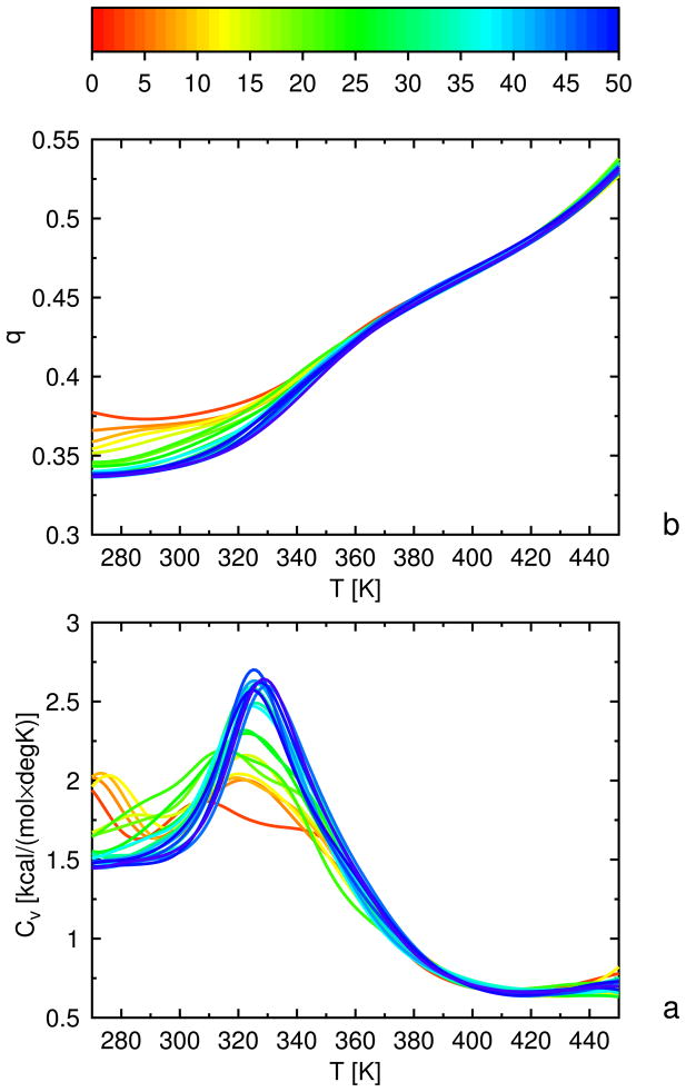
Using canonical ensembles at various temperatures also gives us the advantage of calculating the thermodynamic characteristics of folding and, consequently, of parameterizing the force field to give folding thermodynamics resembling those found experimentally. The process of protein folding is a first-order phase transition and, consequently, the plot of heat capacity vs. temperature should have one clear peak at the folding-transition temperature; this peak should coincide with the jump in native-likeness.46,47 To determine the thermodynamic characteristics of the current UNRES force field,32 for efficient sampling at various temperatures, we recently48,49 included five techniques of multicanonical simulations50 in UNRES/MD, namely replica-exchange molecular dynamics (REMD), multiplexing replica exchange molecular dynamics (MREMD) multicanonical molecular dynamics (MUCAMD), as well as replica-exchange multicanonical (REMUCA) and multicanonical replica-exchange (MUCAREM) molecular dynamics. Of those, the MREMD method turned out to be the most efficient. We found48 that the present UNRES force field32 produces multiple peaks in heat capacity curves; the peaks at the highest temperatures correspond to formation of individual α-helices and are followed at lower temperatures by very broad peaks corresponding to the transition to the native structure. The reason for this is the neglect of the conformational-entropy factor in parameterizing the force field by using the CSA method to generate decoys.
As in our hierarchical protocol of energy-based prediction of protein structure,18,51 UN RES/MD is the first stage of our hierarchy scheme in which all-atom protein-folding trajectories will ultimately be calculated. For protein-structure prediction, we convert united-residue backbones to all-atom backbones first by optimizing the electrostatic and local interactions of the peptide groups,17,52 making use of their simplified representation as point dipoles and, subsequently, we optimize the internal degrees of freedom of the side chains by using a simplified potential53 and a Monte Carlo method. Although this approach is fully energy-based and does not make use of fragment or side-chain libraries or any statistics derived from the PDB, the reconstructed all-atom structures are of the same quality as those obtained using knowledge-based methods.53 In view of this, implementation of the approach developed by Elber and coworkers54,55 to obtain a trajectory, appears to be the most appropriate method to convert the UNRES trajectories to all-atom trajectories. In this procedure,54,55 the action is minimized with appropriate constraints which can be identified with the united-residue conformations at consecutive points of UNRES trajectories.
In this paper, we describe our revised hierarchical-optimization procedure designed to optimize a force field for canonical simulations. To generate the decoy sets, we use the multiplexing replica exchange molecular dynamics (MREMD) method which we recently49 implemented in the UNRES force field. In section 2.1, we recall the UNRES model and force field that was used prior to this work. In section 2.2, we introduce the temperature dependence of UNRES. In section 2.3, we describe the implementation of the MREMD method with temperature-dependent UNRES and the processing of the results to compute thermodynamic quantities. In section 2.4, we describe the implementation of the hierarchical optimization method, developed in our earlier work,25,30–32 in canonical simulations. In section 4, we describe the performance of the new procedure in optimizing the UNRES force field with three test proteins: 1E0L, 1GAB, and 1E0G and, finally, in section 5, we test the predictive power of the force fields parameterized on 1GAB and 1E0G.
2 Methods
2.1 The UNRES force field for global optimization
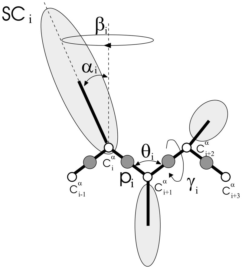
In the UNRES model,17–23,25,27,31,32,37,38,56–58 a polypeptide chain is represented by a sequence of α-carbon (Cα) atoms linked by virtual bonds with attached united side chains (SC) and united peptide groups (p). Each united peptide group is located in the middle between two consecutive α-carbons. Only these united peptide groups and the united side chains serve as interaction sites, the α-carbons serving only to define the chain geometry, as shown in Figure 1. The UNRES force field has been derived as a Restricted Free Energy (RFE) function of an all-atom polypeptide chain plus the surrounding solvent, where the all-atom energy function is averaged over the degrees of freedom that are lost when passing from the all-atom to the simplified system (viz. the degrees of freedom of the solvent, the dihedral angles χ for rotation about the bonds in the side chains, and the torsional angles λ for rotation of the peptide groups about the Cα ··· Cα virtual bonds).21,22 The RFE is further decomposed into factors coming from interactions within and between a given number of united interaction sites.22 Expansion of the factors into generalized Kubo cumulants26 enabled us to derive approximate analytical expressions for the respective terms,21,22 including the multibody or correlation terms, which are derived in other force fields from structural databases or on a heuristic basis.59 The theoretical basis of the force field is described in detail in our earlier paper.22
Fig. 1.
The UNRES model of the polypeptide chain. Dark circles represent united peptide groups (p), open circles represent the Cα atoms, which serve as geometric points. Ellipsoids represent side chains, with their centers of mass at the SC’s. The p’s are located half-way between two consecutive Cα atoms. The virtual-bond angles θ, the virtual-bond dihedral angles γ, and the angles αSC and βSC that define the location of a side chain with respect to the backbone are also indicated.
The energy of the virtual-bond chain is expressed by eq. (1).
| (1) |
Each term is multiplied by an appropriate weight, wx. The term USCiSCj represents the mean free energy of the hydrophobic (hydrophilic) interactions between the side chains, which implicitly contains the contributions from the interactions of the side chain with the solvent. In our earlier work,20,22,31,32 this term was assigned the weight of 1 because the force field was not meant to reproduce any energy scale. This is not the case in our present work in which we want the folding transitions to occur at physiological temperatures and we, therefore, also assign a weight to the USCiSCj terms. The term USCipj denotes the excluded-volume potential of the side-chain – peptide-group interactions. The peptide-group interaction potential is split into two parts: the Lennard-Jones interaction energy between peptide-group centers ( ) and the average electrostatic energy between peptide-group dipoles ( ); the second of these terms accounts for the tendency to form backbone hydrogen bonds between peptide groups pi and pj. In previous versions of the UNRES force field,20,22,25,27,31 we grouped and together and assigned a common weight to them; however, this is not possible after introducing temperature dependence, which is described in the next section. Utor, Utord, Ub, and Urot are the virtual-bond-dihedral angle torsional terms, virtual-bond dihedral angle double-torsional terms, virtual-bond angle bending terms, and side-chain rotamer terms; these terms account for the local propensities of the polypeptide chain. The terms represent correlation or multibody contributions from the coupling between backbone-local and backbone-electrostatic interactions, and the terms are correlation contributions involving m consecutive peptide groups; they are, therefore, termed turn contributions. The correlation contributions were derived21,22 from a generalized-cumulant expansion26 of the restricted free energy (RFE) of the system consisting of the polypeptide chain and the surrounding solvent. The multibody terms are indispensable for reproduction of regular α-helical and β-sheet structures. In the latest version of UNRES,32,37 we use only the multibody terms up to order 4; we found that neglecting higher-order terms does not impair the performance of the force field, while reducing the cost energy evaluation by at least 30 %. The terms Ubond(di), where di is the length of ith virtual bond and nbond is the number of virtual bonds, are simple harmonic potentials of virtual-bond distortions;38 they have been introduced recently for molecular-dynamics implementation.
The internal parameters of , Utor, Utord, , and were recently derived by fitting the analytical expressions to the RFE surfaces of model systems computed at the MP2/6-31G** ab initio level27,57 while the parameters of USCiSCj, USCipj, Ub, and Urot were derived by fitting the calculated distribution functions to those determined from the PDB;20 work is currently in progress to obtain these parameters from quantum mechanical ab initio calculations of the potentials of mean force of appropriate model systems. The w’s are the weights of the energy terms, and they can be determined only by optimization of the potential-energy function, which is the subject of the present paper.
2.2 Introducing temperature dependence of the UNRES force field
The UNRES force field has the sense of a restricted free energy and, as such, should depend on temperature. Thus far, we have ignored this issue, because we defined the solution of the protein-folding problem as that of finding the global minimum the effective energy function, and were not considering temperature-induced unfolding or aggregation. As mentioned earlier, this corresponds to sampling at temperature 0 K. However, UNRES was parameterized to locate native-like structures which, in reality, are stable at physiological temperatures as global potential-energy minima; therefore, we can regard the bottom of the earlier-UNRES energy surface as corresponding to structures at physiological temperature which makes this force field good for protein-structure prediction without having to take temperature dependence into consideration. When thermodynamics of folding is to be reproduced, the temperature dependence of the UNRES force field (as well as of any other coarse-grained force field which is, in principle, defined as a free-energy function) must be considered. To realize this, we recall the definition of the UNRES force field as a free energy of a given coarse-grain conformation defined by the primary degrees of freedom collected in the vector X with integration over the secondary degrees of freedom y (eq 2).22
| (2) |
where E (X; y) is the energy of the system described by the primary degrees of freedom X and the secondary degrees of freedom y calculated at the all-atom level, T is the absolute temperature, R is the universal gas constant, Ωy is the subspace corresponding to the secondary degrees of freedom y, Vy is the volume of this space, and dVy is the volume element.
To derive the UNRES force field, eq 2 was expanded22 into factors involving a gradually increasing number of components of the all-atom energy E(X; y), and each factor was expanded into the Kubo cumulant26 series [i.e., in powers of (RT)−1]. Details of the approach are provided in ref 22. The first non-zero cumulant term of a factor of order n (i.e., containing n component energies) starts from (RT)−(n−1). Thus, in general, the UNRES force field can be written as eq 3.
| (3) |
where N is the maximum order of the factors considered, i labels the factors of the same order, mn is the number of energy terms corresponding to factors of order n, is the highest-order cumulant considered in the expansion of a given factor, and is the jth term in the cumulant expansion of the ith factor of order n. In the UNRES force field, we use only the lowest non-zero cumulants,22 and is equal to n except in the expansion for the average energy of the peptide-group interaction ( ) where the first-order cumulant vanishes22,27 and, consequently, . It should also be noted that the terms are simply average energies of interaction, as demonstrated in ref 22. Table 1 summarizes the orders of the factors and the orders of the lowest non-zero cumulants corresponding to all terms of eq 1. Based on eq 3 and Table 1, it can be seen that the multibody terms which control the formation of organized secondary-structure elements in UNRES (i.e., α-helices, β-sheets, and turns)22 vanish fast with increasing temperature, as should be expected. It can, therefore, be expected that ignoring their dependence on temperature leads to bad prediction of folding thermodynamics; in fact, in section 4.2, we will demonstrate that the resulting overly-large contributions from the multibody terms at high temperature and the resulting over-stability of secondary structure at high temperature is the reason for the appearance of multiple peaks in heat capacity curves calculated with UNRES.
Table 1.
Order of factors and lowest non-zero cumulants corresponding to UNRES energy termsa
| Term | N | ||
|---|---|---|---|
| USCiSCj | 1 | 1 | |
| USCipi | 1 | 1 | |
| Ub | 1 | 1 | |
| Ubond | 1 | 1 | |
| Urot | 1 | 1 | |
|
|
1 | 1 | |
|
|
1 | 2 | |
| Utor | 2 | 2 | |
| Utord | 3 | 3 | |
|
|
3 | 3 | |
|
|
4 | 4 | |
|
|
5 | 5 | |
|
|
6 | 6 | |
|
|
3 | 3 | |
|
|
4 | 4 | |
|
|
6 | 6 |
Based on Table 1, it would seem that introducing temperature dependence is straightforward and that the respective terms should be scaled by fn(T) = (To/T)n−1 where n is the order of the first non-vanishing cumulant in the expansion of the corresponding factor and To is an arbitrary reference temperature; we set To = 300 K. However, this modification of the UNRES force field does not reflect the actual dependence of the factors on temperature; at low temperatures the factors computed from the respective configurational integrals (eq A-3 of ref 27) increase with decreasing temperature slower than the respective inverse power of temperature. Consequently, instead of scaling the cumulant-based terms by powers of the inverse of absolute temperature, we tentatively introduce the scaling factors defined by eq 4.
| (4) |
For n > 1, the factors fn(T) defined by eq 4 are approximately equal to 1.127 (To/T)n−1 for T ≫ To, i.e., they reflect the fact that only cumulants of the lowest order corresponding to a given UNRES energy term contribute to a respective factor. The higher the order of a multibody term, the faster will it vanish with temperature which, as we will demonstrate in the section 4.2, eliminates undesirable peaks in the heat capacity at high temperatures corresponding to premature formation of secondary-structure elements with the UNRES force field developed prior to this work.32,37 At T = To = 300 K, the scaling factors are equal to 1 and, for T < To, fn increases with decreasing temperature slower than powers of the inverse of temperature. The exact temperature dependence of the components of the UNRES energy function (in lieu of eq 4) will be the subject of our future work.
With the scaling factors defined by eq 4 and with the values of based on the last column of Table 1, the restricted free energy of polypeptide chains in the UNRES approximation can be expressed as eq 5 where X denotes the variables defining the conformation of a polypeptide chain in the UNRES approximation.
| (5) |
The term Uo(T) corresponds to the reference free energy at a given temperature and can be approximated by the free energy of an ideal gas of M molecules, M being the number of secondary degrees of freedom (the dimension of the vector y of eq 2). As such, it contributes only a constant factor to the heat capacity. Therefore, we omit Uo from eq 5 in the present work.
The analytical expressions for and have been derived as the lowest-order non-vanishing cumulants,17,21,22 those for Utor and Utord are simple Fourier expansions in one or two consecutive virtual-bond dihedral angles γ, respectively, while effective anisotropic Gay-Berne potentials60 were assumed to represent the USCiSCj terms,19 all-repulsive Lennard-Jones-like potentials were assumed to represent the USCipj terms,18,20 the negatives of the logarithms of sums of Gaussians (derived based on PDB statistics) were assumed to represent the Ub, and Urot terms,20 and simple harmonic potentials were assumed to represent Ubond.38
2.3 Sampling and computing thermodynamic quantities with the temperature-dependent UNRES
In this study, we use the multiplexing replica-exchange molecular dynamics (MREMD) method to sample the conformational space of UNRES chains. The replica-exchange method and its multiplexing variation are described in the literature,50,61–63 and its implementation in the previous version of UNRES is described in our recent work.48,49 Therefore, here we provide only a brief description and the modification introduced to account for the temperature dependence of the force field.
In the REMD method,50,61–63 M canonical MD simulations are carried out simultaneously, each one at a different temperature. Initially, the temperatures increase with the sequential number of simulations (trajectories). After every m steps, an exchange of temperatures between neighboring trajectories (in the order from 1 to M) is attempted, the decision about the exchange being made based on the Metropolis criterion. With a temperature-dependent force field, the Metropolis criterion is defined by eq 6.
| (6) |
where βi = 1/RTi, Ti being the temperature corresponding to the ith trajectory, and Xi denotes the variables of the UNRES conformation of the ith trajectory at the attempted exchange point. If Δ ≤ 0, Ti and Ti+1 are exchanged, otherwise the exchange is performed with probability exp(−Δ). It should be noted that eq 6 reduces to eq 7 (from ref 50), if U does not depend on temperature, i.e., if U is energy and not restricted free energy.
| (7) |
The multiplexing variation of the REMD method (MREMD)64 differs from the REMD method in that several trajectories are run at a given temperature. Each set of trajectories run at a particular temperature constitutes a layer. Exchanges are attempted not only within a single layer but also between layers. In our very recent study,49 we demonstrated that such a procedure increases the power of REMD very considerably, and convergence of the thermodynamic quantities is achieved much faster.
The MREMD method, although very powerful, does not help if the initial-guess force field does not locate any native-like structure in the MD runs, as happens with the β-protein 1E0L and the 4P force field,32 in which case only non-native α-helical structures are found.40 In such cases, it is necessary to implement umbrella sampling with restraints driving the simulation towards native-like structures. The restraints that we implemented are based on the Q-measure of similarity of the distances in two conformations, which is a modified version of the respective quantity introduced by Wolynes and coworkers65 The value of Q varies from 1 for identical structures to 0; therefore, we also define a conjugate quantity q = 1−Q which, like the RMSD, is equal to 0 for identical structures. Specifically, we define Qi (eq 8) and the conjugate quantity qi (eq 9) as a measure of the similarity of the ith fragment of the chain of the conformation under study to its counterpart in the experimental structure; it should be noted that the fragment can be equal to the entire molecule. To quantify the similarity of the distances of fragments i and j (i.e., the similarity of the packing of these two fragments to that in the experimental structure), we define Qij and the conjugate quantity qij (eqs 10 and 11).
| (8) |
| (9) |
| (10) |
| (11) |
where {i} and {j} are the sets of residues constituting fragment i and j, respectively (we note that the fragments do not have to be contiguous; e.g., we can consider a β-sheet composed of two non-sequential strands as a fragment), Ni is the total number of distances (both between the Cα atoms and between the SC pseudo-atoms) in fragment i, Nij is the number of distances between the atoms of fragments i and j, m is the minimum separation of residues in the amino-acid sequence at which the distances are calculated (we set m = 3), or dSCkSCl denotes the distance between the α-carbon atoms or side chains of residues k and l, respectively, of the conformation under consideration, and the same quantities with the nat superscript denote the distances in the experimental structure. Both Q and q vary from 0 to 1. Q = 1 (q = 0) if the conformation considered is the experimental structure and Q < 0.5 (q > 0.5) indicates that the structure considered and the experimental structure are grossly dissimilar. The quantity q has a great advantage over RMSD or distance RMSD in that it assigns larger weights to distances similar to those in the native structure than to those dissimilar. Also, because the standard deviations of the Gaussians are proportional to the distances in the experimental structure, the deviations from small (contact) distances count more than the deviations from large distances in the experimental structure.
The restraint potentials (introduced to confine the simulated conformations to a given native likeness) are defined in terms of q by eq 12.
| (12) |
where qo is the center of the restraint and k is the respective force constant; we implemented k from 0 to 100, and qo from 0 to 0.7, because q rarely exceeds 0.8. The restraints defined by eq 12 can be imposed on the q of the whole molecule or on the q’s computed over pairs of fragments. We will denote the complete energy function used in the jth simulation by Vj (given by eq 13) to distinguish it from the UNRES energy function U.
| (13) |
where Urestr;j denotes the set of restraining potentials (of the form given by eq 12); we also identify the possible dependence of the UNRES energy function on temperature (section 2.2) and βj = 1/RTj where Tj is the absolute temperature of the jth simulation.
In principle, simulations carried out with different sets of restraints [i.e., qo or k in eq 12 can be combined in a single MREMD run which can involve exchanges not only of temperatures but also of total energy functions (including the restraint potentials50]. In the present work, however, we carried out a separate MREMD simulation for each set of restraints, and the replicas involved only different temperatures.
To compute the averages from the results of simulations carried out at different temperatures and restraints, we used the histogram-reweighting technique known as the Weighted Histogram Analysis Method (WHAM).66 Here, we modified the algorithm described in ref 66 to process individual conformations. Given m simulations (termed as windows) differing in temperatures or energy functions, we solve self-consistent equations (eqs 14 and 16) for the probabilities (Pi) of all conformations and the total dimensionless free energies (fk) of all windows
| (14) |
| (15) |
| (16) |
where N is the total number of conformations. The quantity ωi can be considered as the entropy of the ith conformation; it should be noted that ωi does not depend on temperature because the sum in eq 15 runs over all β’s and, consequently, over all temperatures. Equations 16 and 14 can be obtained from equations 19 and 21 of ref 66 if individual conformations instead of distributions of conformation-dependent quantities are considered; these equations result in distributions of conformation-dependent quantities identical to those obtained by solving equations 19 and 21 of ref 66. It should be noted that the entropies of eq 15, calculated by solving self-consistent equations 14 and 16, are valid only within the ensemble of conformations taken into account when solving the WHAM equations; if the set is expanded by adding the results of new simulations, the WHAM equations must be solved again and new entropies calculated.
Once the entropies ωi have been computed with eqs 14 – 16, any ensemble average of a quantity A corresponding to any subset of conformations of the set processed by WHAM at temperature T and with the UNRES potential-energy function U can be computed from eq 17. It should be noted that Urestr of eq 12 must now be omitted from V in order to obtain unbiased averages based only on U.
| (17) |
where {X} denotes the subset of conformations and Xi denotes the variables describing the ith conformation of the subset and the notation {U} indicates that 〈A〉 is a functional that depends on the UNRES energy function U. Z is the partition function defined by eq 18.
| (18) |
Based on eq 18, we define the free energy of any subset {X} of conformations obtained in simulations processed with a given WHAM round by eq 19. Because our optimization procedure is based on optimizing free-energy gaps (differences in free energy between two neighboring levels) between subsets of conformations characterized by different native-likeness (levels),25 eq 19 is of key importance.
| (19) |
We identify the functional dependence of 〈A〉 and F on the UNRES energy function U.
The physical interpretation of the dependence of the UNRES energy function on temperature is that each UNRES conformation corresponds to a collection of microstates with identical coarse-grain variables. We term such states as mesostates. Because of the dependence of the composition of the mesostates on temperature, the internal energy E is not the Boltzmann average over the energies of the microstates. Instead, it contains the temperature derivatives of the energies of the UNRES conformations as well as the Boltzmann average of the energies of the UNRES conformations, as in eq 20. To make the connection to thermodynamics apparent and also to obtain a folded formula, we use T and not β = 1/RT as variable.
| (20) |
Likewise, the heat capacity Cv of the system is not defined as the variance of energies of the UNRES conformations but, instead, is expressed by eq 21.
| (21) |
with
| (22) |
where 〈…〉T denotes the average of a quantity with Boltzmann weights equal to exp(ω – U/RT).
2.4 Hierarchical optimization method to obtain a force field for canonical simulations
The background of the hierarchical optimization method to obtain force fields for global optimization and its application to the UNRES force field17–25,27,56,57 is described in our earlier work.25,30–32 In references 30 and 31, the hierarchical optimization method is also compared to the approaches developed by other authors. The new procedure for optimizing the force fields for canonical simulations is described below.
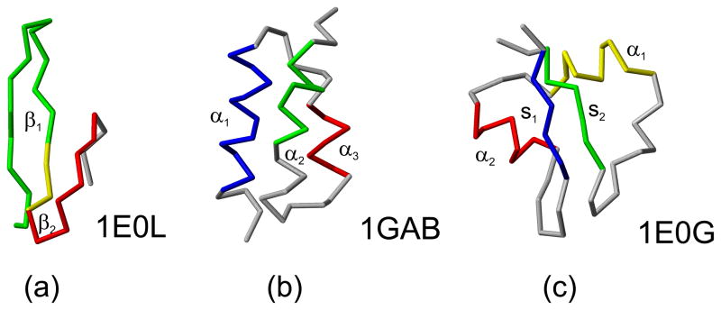
As in our earlier work,25,30–32 we define the elementary fragments of the molecule. These are usually secondary-structure elements. Subsequently, we define the hierarchy levels of the protein in terms of elementary fragments. The order of formation of native-like structure with increasing level number should follow the folding pathway if such information about the respective training protein is available. Otherwise, the optimal order of native-like structure formation can be deduced by trial-and-error as done in our earlier work.31,32 First, the contiguous elements (α-helices or β-hairpins) are selected as elementary fragments and higher hierarchy levels are constructed by assembling them gradually. If some of the elementary fragments or their aggregates persistently fail to appear in probable conformations, or if optimization fails to progress, the choice is revised by removing weakly stable structural elements from lower levels of the hierarchy to higher levels; such a modification assumes that their formation is induced by favorable interactions with the other, already formed, elements of the structure. For example, when optimizing the force field using 1E0G as a training protein,31 we initially assumed that the two-stranded β-sheet (see Figure 4 for the experimental structure of this protein) is formed as a stand-alone element. However, with such a choice, we failed to optimize the force field to locate the native-like structure as the lowest in energy. Only after assuming that each of the strands must develop favorable interactions with the adjacent α-helix prior to β-sheet formation did we optimize the force field with success. An improper definition of hierarchy levels not only makes optimization difficult but also results in a weakly transferable force field with low prediction capability. We proved this statement both by using 12-bead models of polypeptide chains on cubic lattice30 and by comparing different hierarchies designed for the training proteins considered in our earlier work.31,32 For 1IGD, for example, which consists of an N-terminal and a C-terminal β-hairpin forming a four-stranded β-sheet and packed against the middle α-helix, our initial hierarchy assumed formation of any of the three secondary-structure elements at level 1, pairs of any two secondary-structure elements packed against each other level 2, and the complete structure at level 3. The resulting force field was overwhelmingly biased towards β-structure because the N-terminal β-hairpin is not stable alone but only in the context of the C-terminal β-hairpin which can form as a stand-alone element.67 The force field optimized with a hierarchy designed according to the experimental information,67 in which the C-terminal β-hairpin formed first and the N-terminal β-hairpin last, and only after the remaining part of the structure was ready, resulted in a force field which, although optimized using a single training protein, was capable of predicting the structures of a variety of α and α + β proteins and even some β-proteins.31
Fig. 4.
The experimental structures of (a) 1E0L, (b) 1GAB, and (c) 1E0G. The native-like elements considered in the hierarchical optimization are both color-coded and marked with symbols used in the text. For 1E0L, the part of the chain shared by β1 and β2 is colored yellow. The MOLMOL software74 has been used to draw the pictures.
In our earlier work,31 we defined fragments by either of three criteria or a combination thereof: (i) based on the fraction of residues with the same secondary structure as in the corresponding fragment of the experimental structure, or (ii) based on the fraction of contacts in a fragment matching those in the corresponding fragment of the experimental structure (fraction of native contacts) or (iii) based on the similarity of local structure or RMSD from the corresponding part of the experimental structure. The similarity of packing of pairs of fragments was defined in terms of the fraction of inter-fragment native contacts or the RMSD of the pair of fragments from that in the experimental structure. The similarity of a cluster composed of more than two fragments was defined in terms of RMSD from the corresponding part of the experimental structure. The fraction of native contacts is a good measure of similarity when the structures considered are energy minima as in our earlier work.31,32 However, we found that, when conformations from MD trajectories are analyzed using the fraction of native contacts as a measure of native-likeness, too many apparently native-like structures are left out. In most cases, we, therefore, replaced the fraction of contacts with the criterion based on q defined by eq 9 for fragments and by eq 11 for pairs of fragments; a fragment or pair of fragments is considered to be native-like if qi<qcut or qij < qcut, respectively, where qcut ranges from 0.3 to 0.5. Only when the appearance of an appropriate contact pattern between peptide groups was critical for proper definition of α-helices or β-sheets, did we use the old definition31 based on fraction of native contacts.
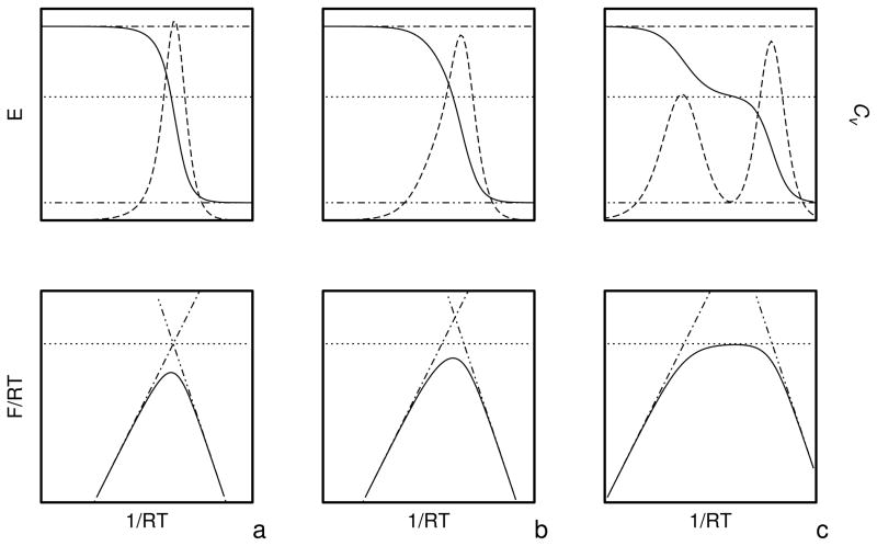
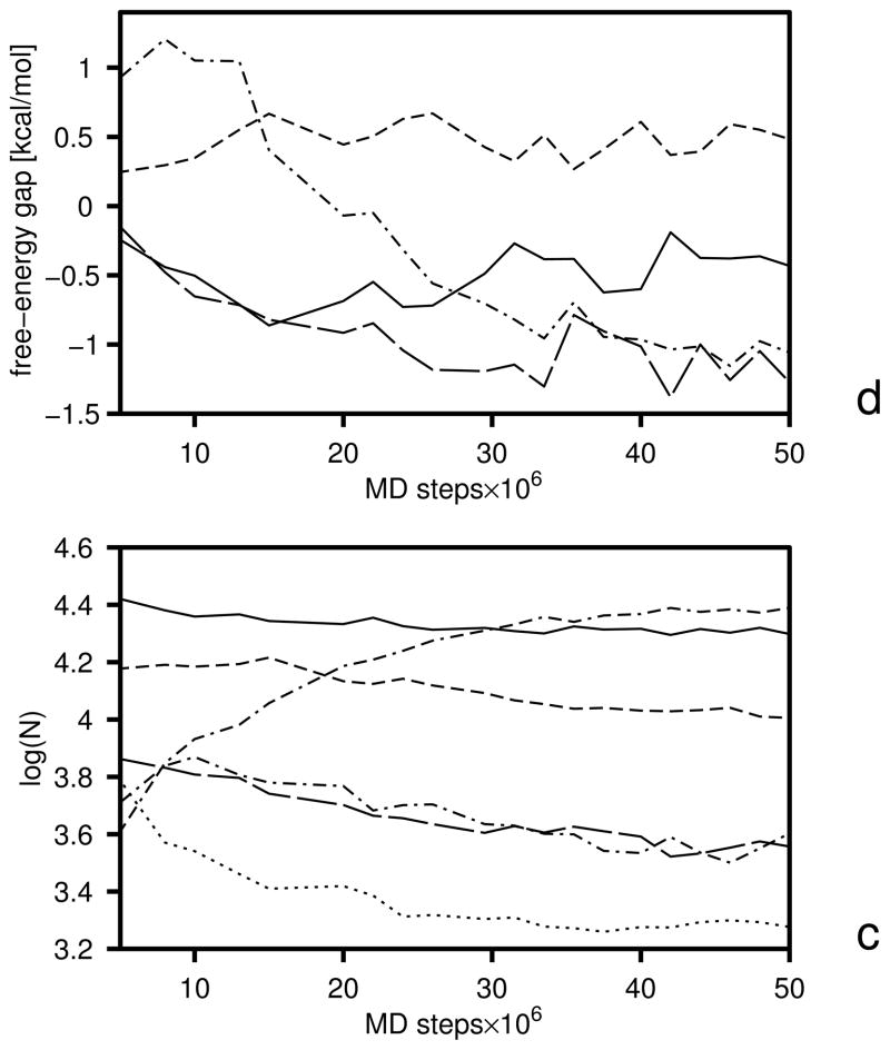
As in our earlier work,25,31,32 we calculate the free energies of the hierarchy levels. However, we use eq 19 as opposed to a simple Boltzmann summation over the low-energy conformations found by CSA that had been used in our earlier work.25,31,32 Equation 19 provides reliable values of the free energies if the temperature is between the lowest and the highest temperature used in the MREMD sampling run to generate the decoy set. Optimization is aimed at achieving appropriate free energy relations between levels: below the transition temperature the free energy should decrease with increasing native likeness, near the transition temperature the free energies of all levels should be equal, and above the transition temperature the free energy should decrease with decreasing native likeness. If the free energies of all levels converge at a single temperature, the folding transition is highly cooperative, and the heat capacity will have a single peak whose height will depend on the slope of the temperature dependence of the free energy gaps near the transition point. Conversely, if the temperatures of transitions between consecutive levels occur at significantly different values (as happens when the UNRES force field is parameterized using CSA-generated decoys in which formation of secondary-structure elements precedes packing of fragments), multiple peaks appear in the heat capacity. Intermediate situations are characterized by a single but broad peak in heat capacity. The above considerations are illustrated in Figure 2 in which schematic plots of selected thermodynamic quantities of a system with three hierarchy levels: level 0 (non-native), level 1 (intermediate) and level 2 (native) are presented for three different patterns (a, b, and c) of the relationship between the free energies of the levels. The dimensionless free energy of level 0 depends on 1/RT with positive slope near the transition point (or depends on T with a negative slope), that of level 1 depends on 1/RT with zero slope, and that of level 2 with a negative slope (or on T with a positive slope) and, consequently, F/RT has a maximum at the transition point. The free energy of level 0 can be regarded as the negative of the free-energy gap between levels 0 and 1 and that of level 2 can be regarded as the free-energy gap between levels 1 and 2 It should be noted, however, that the slope of the dependence of F/RT or F on temperature depends on the origin of the UNRES energy (U) and entropy (ω) scale of the mesostates and, consequently, the slopes near the transition temperature might be all positive or all negative and the free energy might not possess a maximum. However, if the slope of the dependence of the free-energy gaps are the same, the mean-energy and heat-capacity curves (the upper panels in Figure 2) do not change. It should be noted that such ordering of the free energies of the levels, as depicted in Figure 2a and b, also assures that the phase transition in terms of heat capacity will be correlated with the jump in native likeness; if levels are carefully defined and each one is characterized with an approximately constant average q (over the whole molecule), q will jump from values characteristic of non-native structure to those characteristic of native-like structures. Obviously, these remarks pertain only to ideal situations in which the levels are composed of very similar conformations and no phase transition occurs within levels.
Fig. 2.
Schematic plots of the variation of the free energy (lower panels), energy (upper panels, solid lines), and heat capacity (upper panels, dashed lines) of models of three protein systems (a, b, and c) with three hierarchy levels: 0 (non-native), 1 (intermediate), and 2 (native); (a) with the free energies of all three levels intersecting at the folding-transition temperatures, (b) intersecting at different but close temperatures and (c) intersecting at significantly different temperatures. The horizontal lines in the upper panels are the energies of conformations at level 0 (dot-dashed lines), level 1 (dotted lines), and level 2 (dash-double-dotted lines); the straight lines in the lower panels with line styles as above, show the variation of the free energies of each of the levels with temperatures. For clarity, the energies of the individual levels are assumed to be independent of temperature (i.e., all microstates of the same level have the same energy) in the range of temperatures considered. When the free-energy curves of the levels intersect at exactly the same temperature (a), the heat-capacity peak is sharp; it becomes broader when the points of intersection diverge (b), to split, finally, into two separate peaks when the difference between the intersection points becomes large (c). All units are arbitrary and, therefore, no scale is shown on the axes.
Based on the above considerations, we might have defined a target function for minimization consisting of penalty terms for free-energy gap violation as in ref 31, as given by eq 23.
| (23) |
with
| (24) |
where i and j indicate level numbers, ({i} denoting the conformations of level i), β = 1/RT and the temperatures run from below to above the transition point, while and are the lower and the upper bounds, respectively, of the free energy gap between levels i and j; we set and negative for T< Tc where Tc is the transition temperature, and where δ is of the order of 0.5 kcal/mol at the transition temperature, and and positive with and gradually increasing with the temperature for T > Tc. The first sum is taken over all training proteins.
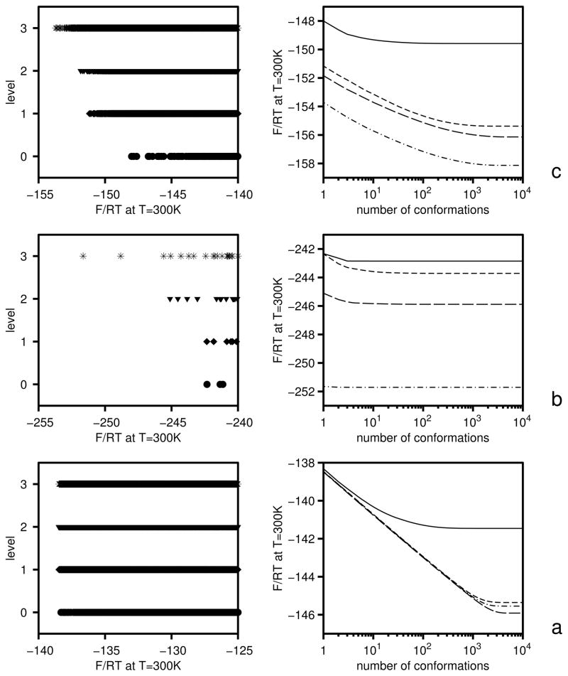
However, such unrestrained optimization of energy-function parameters is dangerous because the distribution of the weights of conformations within levels [equal to exp(ωi− βUi)] can become very different from the distribution corresponding to the initial RFE function (Uo) with which the decoy set was generated. A situation that occurs frequently is separation of one or a few “leader” conformations which acquire outstandingly high weights during the process of optimization and, therefore, make overwhelming contributions to the respective free-energy gaps. This effect is illustrated on the left side of Figure 3a and b where the linear plots of the distributions of the conformations of the 1GAB protein at consecutive levels before (a) and after (b) optimization are presented; this effect is also illustrated on the right side of Figure 3a and b where the plots of the partial free energies of consecutive levels before (a) and after (b) optimization are presented. It can be seen that, before optimization, the points in Figure 3a corresponding to individual conformations are indistinguishable and form thick lines; this means that the respective distributions are compact. This is understandable because the UNRES energy function is the same as that which has been used in the MREMD simulations of the conformational ensembles. Except for level 0 (non-native), about 1,000 conformations contribute nearly equally to the free energies of the levels, which is manifested as almost linear shapes of the plots on the right side of Figure 3a. After unrestricted optimization (eq 23), individual conformations are clearly seen on the low-free-energy part of the linear plots (left side of Figure 3b); in particular, the leader conformation of level 3 (the native-like level) is separated by about 3RT units from the next one which is separated by about the same F/RT gap from the next conformations. A similar, although less severe situation can be observed for levels 0, 1, and 2. This separation of leader conformations from the rest of the ensemble is clearly reflected in the plot of F/RT as a function of the number of contributing conformations (the right side of Figure 3b); it can clearly be seen (on the left side of Figure 3b) that only the two leader conformations contribute significantly to the free energy of the native-like level and less than 10 conformations contribute to the free energies of the other levels. Although the levels seem to be very well ordered according to free energy, this has been achieved only at the expense of forcing a few and, therefore, accidental conformations to be low in the free energy. The predicted ordering of the levels and, consequently, the optimized parameters of the UNRES energy function are, therefore, unreliable. MREMD simulations with the UNRES energy function optimized with features as shown in Figure 3b usually result in completely different free-energy relations than those predicted by optimization of the target function defined by eq 23.
Fig. 3.
Illustration of the role of inclusion of the Shannon-entropy term in eq 25 in the last iteration of the optimization of the force field using 1GAB as the training protein (section 4.2). Left panels: linear plots of the dimensionless free energies (U/RT − ln ω) at T = 300 K (with ω defined by eq 15) of the conformations of the 1GAB protein at level 0 (filled circles), 1 (filled diamonds), 2 (filled triangles), and 3 (asterisks); the symbols are seen most clearly in panel b. Only the low-free-energy parts are shown for clarity, and the F/RT span is the same on all three panels for better comparison. Right panels: plots of partial dimensionless free energies calculated by taking only the N lowest-free-energy conformations (where N is the variable of the abscissa) sorted according to U/RT − ln ω. Solid lines: level 0; short-dashed lines: level 1; long-dashed lines: level 2; dash-dotted lines: level 3. (a) Before minimizing the target function, (b) After minimizing the target function without including the Shannon-entropy term. (c) After minimizing the target function with inclusion of the Shannon-entropy term.
To avoid such situations, we add Shannon-entropy68 terms (eq A-5 of the Appendix) to the target function (one for each level); these terms become large when the distribution of conformations within a level changes considerably with respect to the distribution corresponding to the initial RFE function. After including Shannon entropies, the free-energy gaps are satisfied by shifting the UNRES energies of all conformations of a given level by approximately the same value rather than by shifting the energy of one or two leaders. It must be stressed that these Shannon entropies have nothing in common with thermodynamic entropies of the respective sub-ensembles.
The complete target function is given by eq 25.
| (25) |
where is the UNRES energy of conformation k corresponding to the initial energy parameters (with which the decoy sets were generated), and is the partition function of level i calculated with the initial parameters of the UNRES energy function and the other symbols are defined below eq 23. The last set of summations in eq 25 is the Shannon-entropy term whose derivation is presented in the Appendix. The improvement caused by the addition of the Shannon-entropy terms is apparent in Figure 3c; the linear plots in the left panels are compact and a few thousand conformations contribute almost equally to the free energies of all levels except level 0 (non-native). However, the last feature does not deteriorate the quality of the UNRES energy function because conformations of the non-native level are almost absent from the conformational ensemble at T = 300 K.
We also tried to include terms in eq 25 to force the proper dependence of the heat capacity and q on temperature, i.e., the appearance of a single peak in Cv coinciding with the jump of heat capacity. We found, however, that these features can be achieved by careful choice of the hierarchy, the classification of conformations to specific levels, and the appropriate choice of the dependence of the boundaries of the free-energy gaps (the Δ’s in eq 25) on temperature. Therefore, while including such additional terms in the target function might be necessary when more complex proteins are considered, we omit them from the current procedure.
Optimization is carried out in cycles consisting of MREMD runs, WHAM processing of results to calculate entropies of individual conformations (the ω’s of eq 15) and, subsequently, the free energies of the levels of the hierarchy at all temperatures of choice (eq 19), and minimization of Φ of eq 25. The procedure is terminated when all free-energy gaps in the hierarchy are satisfied within the pre-set boundaries at all temperatures and there is a single peak in the heat capacity at the transition temperature. We ignore the appearance of additional peaks at temperatures close to the lowest temperature of the MREMD simulations (typically below 250 K) because the weights of the conformations are not reliable at temperatures close to the boundaries of the temperature range of an MREMD simulation.
2.5 Clustering
Classification of conformations into levels, as described in section 2.4 is possible only when the respective experimental structure is known; this is the situation in force-field optimization. However, when using the new approach for structure prediction, we need a method to group conformations into families and to rank the families. In our earlier approach,24, 37 which was based on global optimization of the potential-energy function, we used the minimal-tree or minimum-variance clustering69, 70 to group families, and ranked the families according to the potential energy of their leaders defined as the lowest-energy conformations of the respective families. In the new approach, we also use clustering to define families of conformations. To save computation time in clustering, we consider only those conformations whose contributions together constitute a fraction of 0.99 to the partition function at the temperature(s) of choice. This particular cut-off value can be set arbitrarily; however, setting a higher value or even including all conformations in clustering did not change the compositions and ranking of clusters except those which have a low probability and, consequently, are unimportant. The temperature is selected as the highest value before the peak in the heat capacity at which MREMD sampling had been carried out. After clustering is accomplished, we compute the fractions of the families in the conformational ensemble at the temperature of choice (or the probabilities of the families), Pi, where i ranges from 1 to the number of families, from eq 26.
| (26) |
where Zi and Z are the partition functions of family i and of the entire ensemble, respectively, {i} denotes the set of conformations that belong to family i, and the other symbols have been defined earlier in this paper. The families are then sorted according to Pi in descending order. If a given number of candidate structures must be selected (as in the CASP exercise), the cut-off in clustering or the clustering method can be adjusted so that the sum of the probabilities of these families is not less than a pre-defined threshold value. A similar procedure to rank the families was designed recently by Gront et al.;71 however, those authors used the numbers of conformations in a cluster without taking into account their weights which, in this work, are computed by using the WHAM procedure.
We select the representative of each cluster in the following manner. First, we superpose all conformations on the one which has the largest Pi (eq 26) among the conformations of this cluster. Then, using the superposed coordinates, we calculate the average conformation using eq 27.
| (27) |
where {I} denotes cluster {I}, r̄i({I}) denotes the vector of the Cartesian coordinates of the average conformation of cluster {I}, rik denotes the Cartesian coordinates of the ith atom of the kth conformation, and the probabilities Pi are defined by eq 26. Finally, we choose that conformation of the cluster as a representative of the cluster which has the smallest RMSD from the mean conformation defined by eq 27.
The RMSD of the cluster representative from the experimental structure selected as described above, is an obvious measure of the quality of the prediction. To estimate the error in the prediction, it is, however, worthwhile to consider the average RMSD over a cluster (ρ̄) defined by eq 28.
| (28) |
where ρk is the RMSD of the kth conformation of the cluster from the experimental structure.
3 Details of calculations
All UNRES/MREMD simulations were carried out with the use of the Berendsen thermostat,72 the implementation of which in UNRES/MD has been described in our earlier paper.39 Consequently, the random and stochastic force were not included. In our earlier work39,40 we have shown that Newton’s dynamics with the Berendsen thermostat leads to faster simulated folding compared to Langevin dynamics, which justifies its use in the present work, where the purpose of the simulations was to obtain converged thermodynamic functions and ensemble averages and not to determine the kinetics of folding. The coupling parameter was assumed to be τ = 1 mtu (where 1 mtu=48.9 fs) as in our earlier work.39 The Velocity Verlet (VV) algorithm73 with the variable time step extension developed in our earlier work38 was used, and the basic time step in integrating the equations of motion was 5 fs. For 1E0L, MREMD simulations were run at 16 temperatures with 5 trajectories/temperature and, for 1GAB, 1E0G, and the proteins used to test the force fields, MREMD simulations were run at 20 temperatures with 16 trajectories/temperature.
The drawings of the structures of the proteins considered in this work were prepared with MOLMOL.74 All graphs were drawn by using the GRI free drawing software (http://gri.sourceforge.net)
4 Results and Discussion
In this section we describe the optimization of the UNRES force field using three training proteins: 1E0L (a three-stranded antiparallel β-sheet), 1GAB (a three-helix bundle) and 1E0G (an α + β protein). The experimental structures of these three proteins and their partition into fragments are shown in Figure 4.
4.1 1E0L as a training protein
1E0L is a 37-residue protein which consists of the 28-residue three-stranded antiparallel β-sheet capped with largely unstructured ends, which form hydrophobic contacts with it. As in our earlier studies in which CSA was used to search conformational space,31, 32 we selected the central 28-residue fragment of this protein, which corresponds to a three-stranded β-sheet (Figure 4a). This fragment has been demonstrated to fold75 experimentally, although its detailed experimental structure is not known; we, therefore, took the structure of the fragment from the crystal structure of the complete 1E0L. Although the native-like β-sheet structure is a global minimum of the F2 and 4P variations of the UNRES force field developed in references 31 and 32, respectively, the native-like structures do not appear in UNRES/MD simulations with these force fields.40 We, therefore, considered this protein as an ideal candidate to test the new procedure of force-field optimization.
With 1E0L we performed two optimization jobs, starting one with the F231 and the other with the 4P force field.32 The objective of the first optimization job was to improve the F2 force field to fold 1E0L in canonical MD simulations. We, therefore, used the original formulation of the UNRES force field as given by eq 1 without introducing temperature dependence. For this reason, we also did not attempt to obtain the folding transition at a physiological temperature. The second optimization job was aimed at obtaining a force field to reproduce the actual thermodynamics of the folding of 1E0L. Because of the small size of the protein and its trivial fold we did not expect either of the force fields to be transferable.
Improvement of the F2 force field (the first optimization job)
With the F2 force field, the typical folding temperatures are about 500 K.39 We, therefore, optimized the gaps at temperatures within the range from 500 K to 700 K aiming at a transition temperature of the order of 600 K. Only the energy-term weights were optimized. The experimental structure of 1E0L and its partition into fragments are shown in Figure 4a. We defined two fragments corresponding to the N-terminal hairpin (referred to as β1) and the C-terminal hairpin (β2) and, based on this partition of the native structure, defined the following hierarchy:
Level 0: Structures with no native hairpin.
Level 1: Both β1 and β2 formed but the RMSD from the experimental structure is greater than 3 Å.
Level 2: Both β-hairpins formed and the RMSD from the native structure is less than 3 Å.
A β-hairpin was considered formed if the fraction of native contacts between peptide groups (defined according to ref 31) was greater than 0.5. Initially, we introduced an intermediate level between levels 0 and 1 of the list above with β1 or β2 formed; however, the population of such structures turned out to be insignificant.
To generate the decoy sets, we carried out restrained MD runs using restraints imposed on the q of the whole molecule with the restraint potential Urestr(q) defined by eq 12. With the original F2 force field,31 we ran 9 windows with qo from 0 to 0.8 spaced at 0.1 intervals to ensure a dense coverage of the conformational space of 1E0L in the generation of the initial decoy set, and then ran 5 windows with qo = 0, 0.2, 0.4, 0.6, and 0.8, respectively in the subsequent two iterations. The optimized parameters were the energy-term weights (eq 1) and the well-depths of the USCiSCj potential. The other parameters were fixed at the values from the F2 force field.31
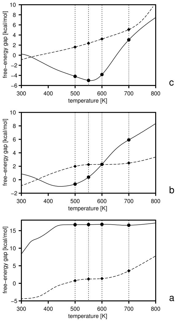
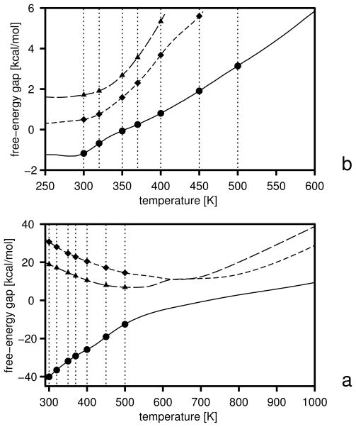
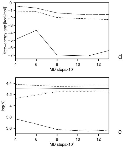
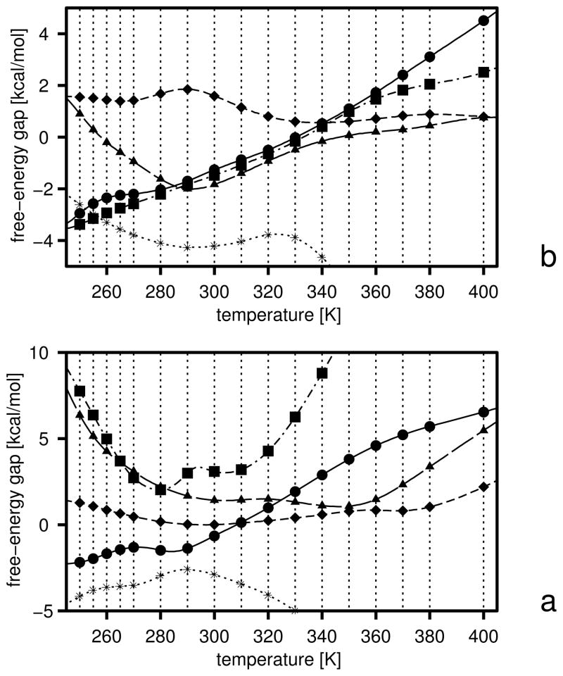
The initial free-energy gaps between levels and the gaps after the first and the second iterations are plotted versus temperature in Figure 5, and the boundaries of the free-energy gaps are summarized in Table 2. The initial and final energy-term weights are collected in Table 3. It should be noted (Table 3) that wSCp, , and decreased after optimization. The decrease of wSCp allows for a closer approach of the peptide groups as encountered in β-sheets, while the decrease of gives less preference to α-helical structures which possess more contacts between peptide groups. Because the weight of the term, which can be considered as a β-structure former,22 is almost unchanged, the optimized force field favors the β-structure more than the original one. The gaps corresponding to iteration 1 and 2 were calculated with the decoy sets generated with the parameters obtained by optimization of the target function defined by eq 25. It can be seen from Figure 5 that the free-energy gaps between levels 0 and 1 moved towards the upper boundaries (shown in Table 2) even after iteration 1 (Figure 5b).
Fig. 5.
Variation of the free-energy gaps (ΔF) between level 0 and 1 (solid lines and filled circles) and levels 1 and 2 (dashed lines and filled diamonds) in optimization of the UNRES force field starting from the F2 force field of ref 31. The gaps at the temperatures included in the target function (eq 25) are shown as filled symbols and the temperatures are marked with thin dotted vertical lines, (a) Initial gaps, (b) gaps after iteration 1, (c) gaps after iteration 2.
Table 2.
Lower and upper bounds of the free-energy gaps (kcal/mol) in optimization of the UNRES force field using 1E0L as a training protein
| T [K] | ||||||||
|---|---|---|---|---|---|---|---|---|
| 500 | −∞ | −10.0 | −∞ | −5.0 | ||||
| 550 | −5.0 | 0.0 | −1.0 | 1.0 | ||||
| 600 | −1.0 | 1.0 | 1.0 | 5.0 | ||||
| 700 | −1.0 | 5.0 | 5.0 | 10.0 |
Lower [marked with superscript (1)] and upper [marked with superscript (2)] boundaries of the free-energy gaps (eq 25). The subscript indicates the levels between which the gap is defined; e.g., is the lower boundary of the free-energy gap between conformations of level 0 and those of combined levels and 2.
Table 3.
Initial and final energy-term weights resulting from optimization of the UNRES force field using 1E0L as a training protein
| weighta | Start from F231 | Start from 4P32 | |||
|---|---|---|---|---|---|
| initial | final | initial | final | ||
| wSC | 1.00000 | 1.00000 | 1.00000 | 0.50099 | |
| wSCp | 2.79405 | 2.28340 | 1.40000 | 1.24684 | |
|
|
0.14581 | 0.06447 | 0.07500 | 0.10612 | |
|
|
0.14581 | 0.06447 | 0.07500 | 0.03294 | |
| wb | 1.95684 | 1.87760 | 1.00000 | 0.13040 | |
| wrot | 0.17010 | 0.44811 | 0.08500 | 0.14337 | |
| wtor | 2.04698 | 2.23279 | 1.00000 | 1.27557 | |
| wtord | 1.69624 | 2.03416 | 0.85000 | 0.76045 | |
|
|
1.21837 | 1.21590 | 0.60000 | 0.78400 | |
|
|
1.84615 | 1.77736 | 0.90000 | 0.75106 | |
|
|
0.02730 | 0.02730 | 0.00000 | 0.00000 | |
|
|
0.00741 | 0.00741 | 0.00000 | 0.00000 | |
|
|
2.91386 | 3.00000 | 1.45000 | 1.31026 | |
|
|
0.73178 | 1.23664 | 0.40000 | 0.27962 | |
|
|
0.02391 | 0.02391 | 0.00000 | 0.00000 | |
In optimization starting from the F2 force field, wSC was fixed at 1.0.
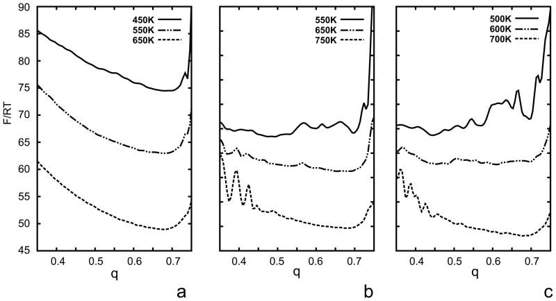
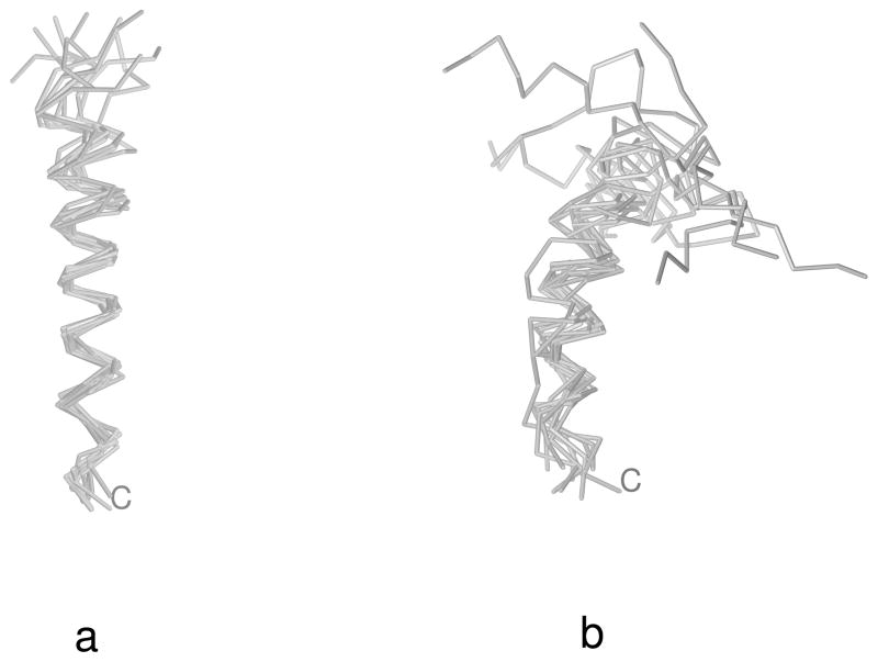
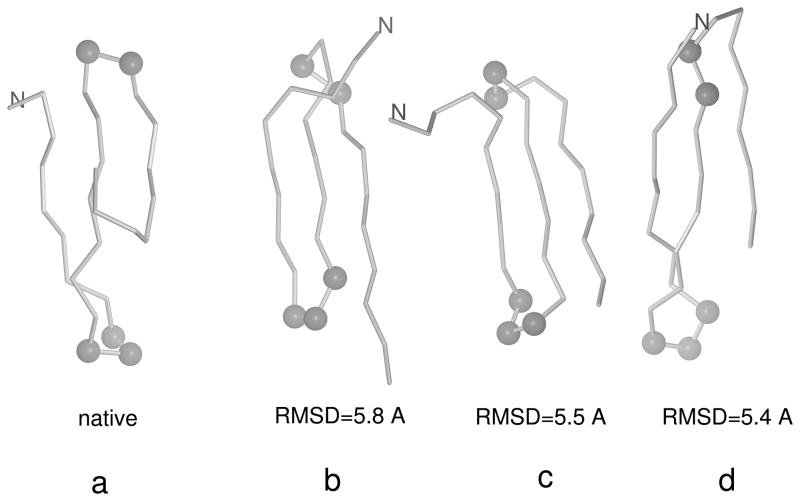
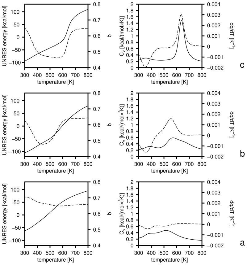
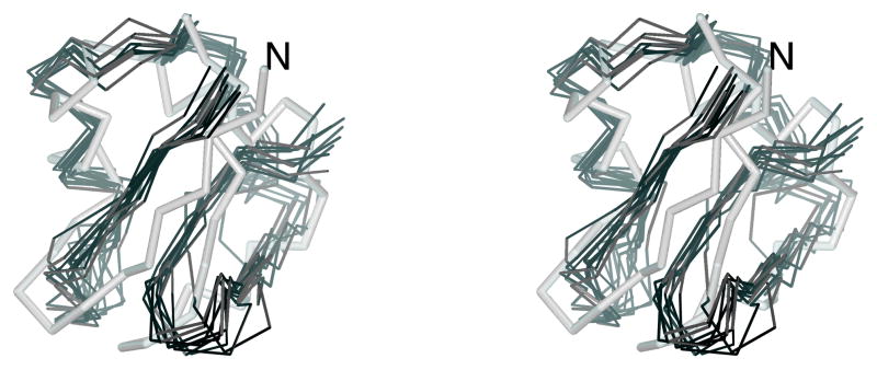
The behavior shown in Figure 5 is reflected in the change of the plots of dimensionless free energy (F/RT) vs. q at selected temperatures (before, near, and after the folding-transition temperature) in iteration 0, 1, and 2, which are shown in Figure 6a–c. The initial profiles of F/RT (Figure 6a) have global minima at q ≈ 0.7; the corresponding structures are largely α-helical at all temperatures as noticed in our earlier work40 and as also shown in Figure 7. The difference between the minimum dimensionless free energy and that at q ≈ 0.4 is about 10 units; such large difference in probability explains why the native-like structures do not appear in simulations. After iteration 1, the global minimum of F/RT at T = 550 K (Figure 6b) occurs at about q = 0.5 (i.e., it corresponds to partially native-like structures); however, there is also a minimum around q = 0.7. After iteration 2, the minimum in q shifts to q = 0.45 (it occurs for T = 500 K) and the minimum at q = 0.7 shifts to somewhat higher free energies (Figure 6c). The free-energy gaps between levels 1 and 2 (Figure 5c) are still positive at temperatures lower than the folding-transition temperature (about 650 K), which means that optimization was not fully successful. However, the structures of level 1 are already three-stranded antiparallel β-sheets (Figure 8), and the reason why they do not belong to level 2 is that the RMSD from the experimental structure is too high. By inspection of the conformational ensemble (Figure 8), we learned that the increased RMSD values were caused by the β-turns being shifted by up to ±3 residues with respect to their native positions. Because the objective of this exercise was to demonstrate that the originally non-predictive force field can be improved and, moreover, we considered only the β-sheet core of 1E0L in optimization, and it is not clear if the β-turns are at the same positions in the truncated sequence as in the full sequence, we did not pursue optimization further. It should also be noted that both β-turns were also shifted with respect to their native positions in the global-minimum structures of 1E0L located with the F2 and the 4P force field.31, 32
Fig. 6.
Variation of the dimensionless free energy (F/RT) of the 1E0L protein with q at selected temperatures in consecutive iterations of the optimization of the UNRES force field starting from the F2 force field of ref 31. (a) Initial, (b) after iteration 1, (c) after iteration 2.
Fig. 7.
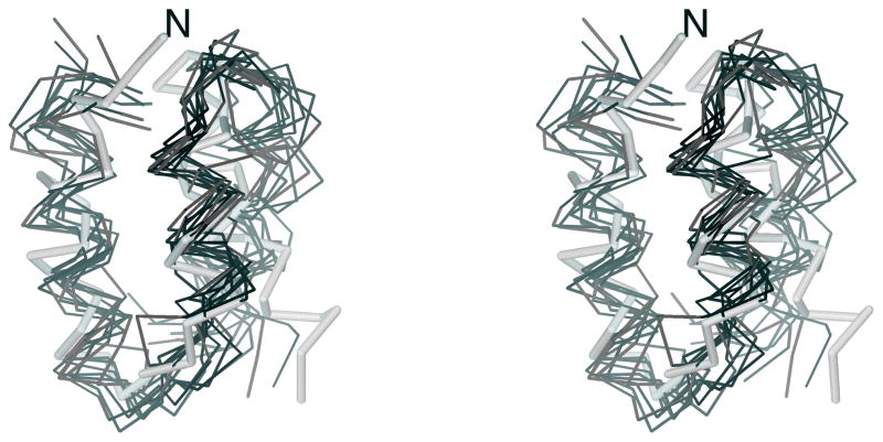
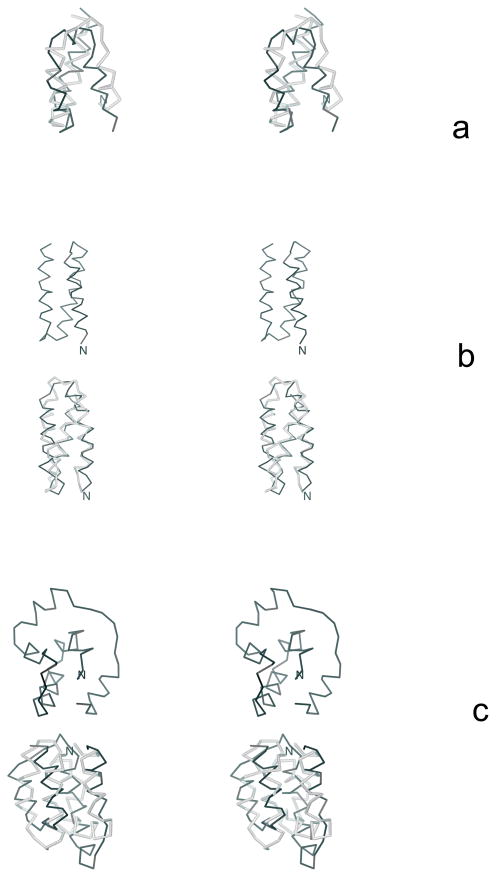
Superposition of the 10 most probable structures of 1E0L calculated by using the MREMD method with the F2 force field31 at T = 300 K (a) and T = 500 K (b). The C-terminus is marked for tracing purposes. The MOLMOL software74 has been used to draw the pictures.
Fig. 8.
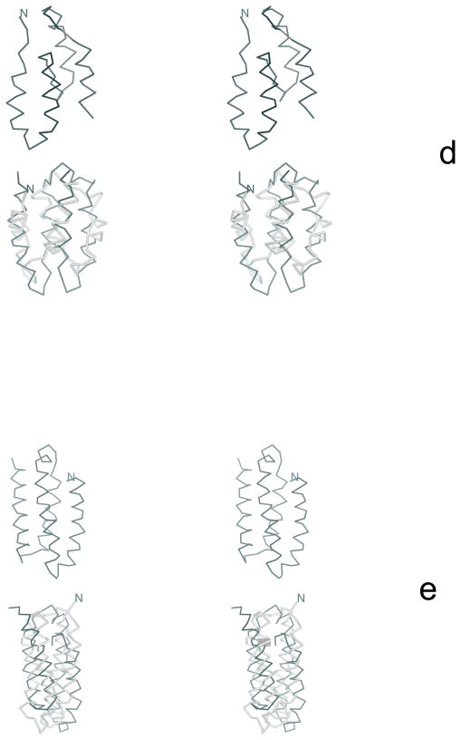
The experimental structure of 1E0L (a) and three most probable structures obtained with the final force field optimized starting from the F2 force field31 (b–d) at T = 600 K. The Cα atoms of the residues involved in the N-terminal γ-turn and the C-terminal β-turn in the native structures are shown as gray spheres. It can be seen that the C-terminal β-turn is shifted or distorted and the C-terminal segment is a part of the β-hairpin in the calculated structures as opposed to the experimental structure; this results in large RMSD values although the topology of the calculated structures is native-like. The N-terminus is marked for tracing purposes. The MOLMOL software74 has been used to draw the pictures.
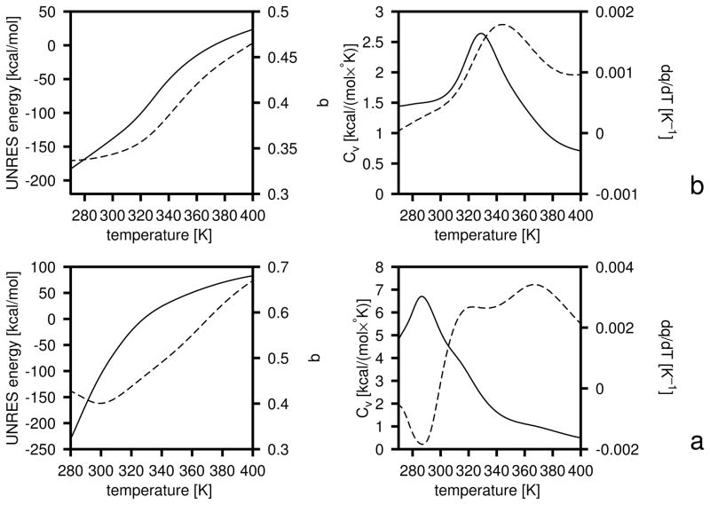
We ran canonical simulations at T = 600 K with the new force fields of iteration 1 and 2; this temperature is lower than the folding-transition temperature for the force field of iteration 2 and is the folding-transition temperature for the force field of iteration 1. The force field of iteration 1 resulted in native-like three-stranded antiparallel β-sheets (with turn positions shifted by up to ±3 residues) in 50 % of the runs and in nearly 100 % of the runs in iteration 2. Canonical runs with the force field of iteration 1 carried out at 500 K (i.e., below the folding-transition temperature), gave poorer performance, which can be explained by the fact that the heat-capacity peak corresponding to that force field is broad (Figure 9b) and, consequently, the force field exhibits some glassy behavior. We, therefore, have demonstrated that the new optimization procedure can produce a force field good enough for canonical folding simulations. This improvement over our old procedure25, 31, 32 which was based on the decoy sets produced by the CSA global-optimization method28, 76 is caused by the fact that our new procedure takes the conformational entropy into account; the entropy was largely ignored in the CSA-based procedure. The native-like structures obtained with the optimized force field have RMSD’s from 2 to 6 Å, the most probable structures having the larger RMSD values in this range. The wide span of RMSD’s occurred because of the shifting of the turn positions and by better packing of the ends of the strands in the calculated structures compared to the experimental structures; example structures at T = 500 K are compared with the experimental structure in Figure 8.
Fig. 9.
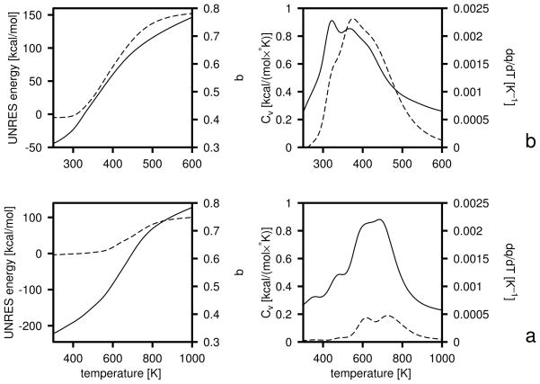
Left panels: plots of the energy (eq 20; solid lines) and q (dashed lines); right panels: plots of the heat capacity (eq 21; solid lines) and dq/dT (dashed lines) of the 1E0L protein in consecutive iterations of optimization of the UNRES force field starting from the F2 force field of ref 31. (a) Initial curves, (b) iteration 1, (c) iteration 2.
It is of interest to analyze the temperature plots of the average energy and the native likeness of the system as well as those of the derivatives of these two quantities with respect to temperature (the heat capacity, Cv and dq/dT). The coincidence of the peaks of Cv and dq/dT (which can be approximated by the variance of q) can be considered to be a condition for a good folder.46 The respective plots are shown in Figure 9a–c. It can be seen that, with the initial parameters of the UNRES energy function (the left column of Table 3), the heat capacity exhibits a broad peak at about T = 550 K and a shoulder at about 400 K (Figure 9a). The high-temperature peak corresponds to the formation of non-native structures with a C-terminal α-helix, and undefined structure in the N-terminal part (Figure 7b), and the low-temperature shoulder to its conversion into a straight α-helix (Figure 7a); this conversion is manifested as a small increase of q at low temperature. The β-structures do not come into play within the range of low temperatures at which the system does not become glassy, although the native-like three-stranded antiparallel β-sheet is the global minimum of the UNRES energy function.31 After iteration 1, only one major peak appears in the heat capacity at 600 K which nearly coincides with the peak in dq/dt (Figure 9b) as well as with the drop of q to about 0.5 at 450 K (Figure 9b). The peak in Cv is broad, i.e., the transition is not sharp; this is reflected in the fact that not all canonical MD runs with the force field of iteration 1 ended up as native-like structures. The increase of q below 400 K to 0.65, coinciding with a small secondary peak in Cv at about T = 400 K, is caused by formation of straight α-helices as dominant structures at low temperatures (such as those shown in Figure 7a). After iteration 2, the peak of the heat capacity becomes sharper and more than twice as high as that of iteration 1. This peak coincides exactly with that in dq/dT as well as with the drop in q to about 0.45 (Figure 9c). These features indicate a clear transition to native-like structures. However, the small peak in Cv below T = 400 K accompanied by an increase of q at low temperatures still remains; the increase of q with decreasing temperatures is connected with the formation of straight α-helices (such as those shown in Figure 7a) at temperatures lower than 400 K.
Derivation of a force field to reproduce the folding thermodynamics of 1E0L (the second optimization job)
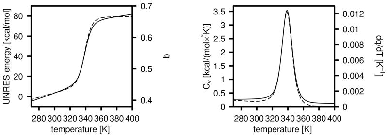
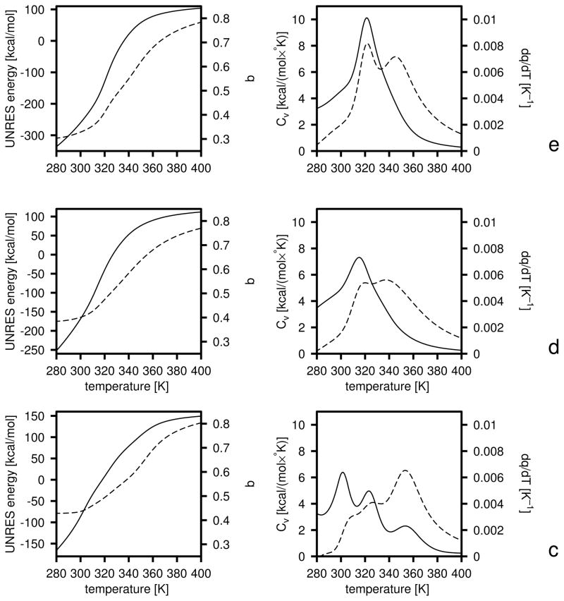
To obtain a force field resulting in a folding transition at physiological temperatures, we repeated the above exercise starting from a modified 4P force field in which all energy-term weights except wbond had been divided by 2 and the parameters of the USCiSCj potentials of eq 1 had been set at the original values determined from the PDB statistics.19 The weights from the 4P force field32 had been divided by 2 because a typical folding temperature with this force field is 800 K40 and, therefore, scaling them down moves it to the range of physiological temperatures. Both the energy-term weights and the well-depths of the USCiSCj potentials were optimized. The initial and final energy-term weights are summarized in Table 3, and the final plots of energy, native likeness as well as those of Cv and dq/dT are shown in Figure 10. As for optimization starting from the F2 force field, it can be seen that wSCp and decreased and, additionally, the weight of the β-sheet former, , increased; consequently, the optimized force field favors the formation of β-structure. It can be seen that the heat capacity has a maximum at a temperature close to T = 350 K, and the half-width of the peak is about 30 K. The peak in the heat capacity coincides with that in dq/dT. If we identify the width of the peak (about 30 K) with the range of temperatures at which the major transition to a native-like structure occurs, both the transition temperature and the range of drop of q are in a very good agreement with those measured experimentally by Gruebele et al.75 for the wild-type and mutants of the WW domain (1E0L). The peak is broader than 10–20 K that is found for typical-size proteins77 because of the small size of the 1E0L fragment, which results in only a marginal thermodynamic stability.
Fig. 10.
Left panel: a plot of the energy (eq 20; solid line) and q (dashed line); right panel: a plot of the heat capacity (eq 21); solid line) and dq/dT (dashed line) for the 1E0L protein, corresponding to the UNRES force field optimized by starting from the scaled 4P force field of ref 32.
It should be noted that, although we have produced a temperature-independent version of the UNRES force field which reproduces a clear folding transition in 1E0L, this is because the secondary structure is inseparable from tertiary structure due to the small size of the protein. In the next example, we demonstrate that, when the tertiary structure arises as a result of packing of secondary-structure elements by means of side chain-side chain interactions, introduction of the temperature-dependent UNRES energy function is necessary to achieve a clear folding transition.
4.2 1GAB as a training protein
1GAB is a 53-residue protein whose major part is a 47-residue-long three-helix bundle fold which extends from Leu6 to Ala53.35 Its experimental structure and partition into fragments is illustrated in Figure 4b. Each α-helix was defined as a fragment; they are referred to as α1, α2, and α3, the numbers running from the N-terminus to the C-terminus.
We defined the following hierarchy:
Level 0: Structures without α2 and without α3.
Level 1: Structures with α2 or α3 formed.
Level 2: Structures with α2 and α3 formed and packed to each other.
Level 3: Structures with all three α-helices formed, packed to each other, and with RMSD from the experimental structure less than 5 Å
This hierarchy scheme assumes that helices α2 and α3 initiate folding, while α1 forms last. Consequently, the presence or absence of α1 at lower hierarchy levels is unimportant. Fragment αi was considered to be a native α-helix if qαi < 0.4, and fragments αi and αj were considered packed as in the experimental structure if qαiαj < 0.4, for each of the helices.
The first round of optimization was carried out with a temperature-independent force field (eq 1). The initial energy-term weights were obtained by dividing the weights of the 4P force field32 by 2 to bring the folding temperature to physiological range) except for wbond which was set at 1 and not varied. The side chain-side chain interaction parameters were set at values determined in our earlier work19 from PDB statistics. Other parameters were the same as in the 4P force field.32 Only energy-term weights were optimized in this round.
As for 1E0L, we carried out restrained MREMD runs to generate decoy sets. We defined four windows centered at qo = 0.0, 0.2, 0.4, and 0.6, respectively with a force constant of kq = 100 kcal/mol×Å2). In iterations 0 and 1, we merged level 1 with level 0 (i.e., the fragment composed of both α2 and α3 level 2) was considered the minimum native-like fragment). The boundaries of the free-energy gaps are summarized in Table 4. The initial and final free-energy gaps after running three iterations) are plotted vs. temperature in Figure 11a and b, respectively while the plots of energy, native likeness, heat capacity, and the temperature derivative of the native-likeness as functions of temperature are shown in Figure 12a and b. The initial and optimized energy-term weights are summarized in Table 5. It can be seen that the values of wSCp and optimized with the temperature-independent force field (the interim1 column in Table 5) are greater than those optimized on 1E0L starting from the 4P force field the last column in Table 3), and the value of is smaller compared to that optimized using 1E0L; consequently, the force field favors α-helical structures.
Table 4.
Lower and upper bounds of the free-energy gaps (kcal/mol) in optimization of the UNRES force field using 1GAB as a training protein. See the legend to Table 2 for explanation of notation.
| T[K] | ||||||||||||
|---|---|---|---|---|---|---|---|---|---|---|---|---|
| 270 | −∞ | −8.0 | −∞ | −3.0 | −∞ | −1.0 | ||||||
| 280 | −∞ | −8.0 | −∞ | −3.0 | −∞ | −3.0 | ||||||
| 290 | −∞ | −8.0 | −∞ | −3.0 | −∞ | −3.0 | ||||||
| 300 | −∞ | −5.0 | −∞ | −3.0 | −∞ | −3.0 | ||||||
| 310 | −∞ | −2.0 | −∞ | −1.0 | −∞ | −1.0 | ||||||
| 320 | −0.5 | 0.5 | −0.5 | 0.5 | −0.5 | 0.5 | ||||||
| 330 | 1.0 | 5.0 | 1.0 | 5.0 | 1.0 | 5.0 | ||||||
| 340 | 2.0 | 10.0 | 2.0 | 10.0 | 2.0 | 10.0 | ||||||
| 350–440 | 2.0 | 50.0 | 2.0 | 50.0 | 2.0 | 50.0 |
Fig. 11.
Variation of the free-energy gaps between level 0 and 1 (solid lines and filled circles) 1 and 2 (short-dashed lines and filled diamonds), and 2 and 3 (long-dashed lines and filled triangles) in optimization of the UNRES force field for the 1GAB protein starting from the 4P force field developed in ref 32. The gaps at the temperatures included in the target function (eq 25) are shown as filled symbols and the temperatures are marked with thin dotted vertical lines, (a) Initial gaps calculated with temperature-independent force field (eq 1), (b) gaps after iteration 3 of the optimization of the temperature-independent force field, (c) initial gaps calculated with energy-term weights corresponding to panel (b) and column interim1 of Table but with temperature-dependent force field (eq 5), (d) gaps calculated with temperature-dependent force field with only energy-term weights optimized, (e) gaps calculated with temperature-dependent force field with energy-term weights and well-depths of the USCiSCj potentials optimized.
Fig. 12.
Left panels: plots of the energy (solid lines) and q (dashed lines), right panels: plots of the heat capacity (solid lines) and dq/dT (dashed lines) of the 1GAB protein in consecutive iterations of the optimization of the UNRES force field. (a) Plots corresponding to the temperature-independent force field and initial parameters, (b) optimized temperature-independent force field after three iterations, (c) energy-term weights determined in part (b) used as initial ones in a temperature-dependent force field, (d) temperature-dependent force field with only energy-term weights optimized, (e) temperature-dependent force field with energy-term weights and well-depths of the USCiSCj potentials optimized.
Table 5.
Initial and final energy-term weights resulting from the optimization of the UNRES force field using 1GAB as a training protein
| weighta | initial | interim1b | interim2c | finald | |
|---|---|---|---|---|---|
| wSC | 1.00000 | 1.16967 | 1.11988 | 1.35279 | |
| wSCp | 1.35000 | 1.77855 | 1.52281 | 1.59304 | |
|
|
0.03400 | 0.95196 | 0.74945 | 0.71534 | |
|
|
0.03400 | 0.11371 | 0.11371 | 0.11371 | |
| wb | 2.08000 | 0.82946 | 1.10857 | 1.13873 | |
| Wrot | 0.08000 | 0.14137 | 0.16147 | 0.16258 | |
| Wtor | 1.50000 | 2.66458 | 1.95687 | 1.98599 | |
| Wtord | 1.45000 | 0.71317 | 1.62540 | 1.57069 | |
|
|
0.03400 | 0.55695 | 0.24313 | 0.16036 | |
|
|
1.00000 | 0.12045 | 0.34502 | 0.42887 | |
|
|
1.20000 | 1.21545 | 1.74649 | 1.68722 | |
|
|
0.70000 | 0.48073 | 0.61716 | 0.66230 |
The initial weights were obtained by scaling the weights of the 4P force field32 by 0.5, except wSC which was set at 1.0. The correlation terms of order higher than 4 were set at zero as in the 4P force field.32
Optimized assuming the UNRES energy function to be independent of temperature (eq 1); parameters of USCiSCj assigned values determined from PDB statistics.19
Optimized assuming the UNRES energy function dependent on temperature (eq 5); parameters of USCiSCj assigned values determined from PDB statistics.19
Final values obtained assuming the UNRES energy function to be dependent on temperature and with the well-depths of the USCiSCj potential included in optimization.
It can be seen (Figure 11b) that levels 0 and 1 are ordered well according to free energy after temperature-independent optimization, while levels 2 and 3 are higher in free energy than level 1 (Figure 11b). Despite this undesirable feature, the optimized force field produces a considerable population of native-like conformations; such structures started to appear in unrestrained MREMD runs already in iteration 2. However, the heat-capacity curves of iteration 2 and 3 still exhibit multiple peaks, and the peak region of the heat-capacity curve is much broader (Figure 12b) compared to the experimental Cv curves determined for a number of proteins.77 The peaks at higher temperatures correspond to the formation of isolated α-helices while that near 320 K corresponds to packing (Figure 12b). Attempts at merging all of the peaks into one by adjusting the limits of the free-energy gaps and also by setting limits on Cv at selected temperatures were unsuccessful. By examining the ensembles at various temperatures, we concluded that the failure to obtain a force field with reasonable thermodynamic properties arises from ignoring the temperature dependence of the multibody terms. The multibody terms, which in UNRES account for the the stabilization of secondary structure, must be sufficiently strong in the region of thermodynamic stability of the entire protein. In temperature-independent UNRES, these terms strongly promote the formation of secondary-structure elements both above and below the folding-transition temperature. Consequently, the secondary-structure elements are stable and stand-alone units. One manifestation of this property of the UNRES energy function of eq 1 is that folding starts from the formation of secondary-structure elements,40, 45, 78 i.e., according to the diffusion-collision model, while folding is known from experiment79–83 to be a highly cooperative phenomenon. The other manifestation is the appearance of additional peaks in Cv above the actual folding temperature (Figure 12b), which correspond to the formation of stand-alone secondary-structure elements. These peaks can, of course, be reduced or eliminated by diminishing the weights of the multibody terms but such an operation severely impairs the stability of secondary-structure elements in the entire range of temperatures. However, it is clear that the requirement of absence of stand-alone secondary-structure elements at temperatures higher than the folding temperature and their appearance and sufficient stability below the folding-transition temperature can easily be reconciled by scaling these weights in a temperature-dependent manner, as shown in eq 5. This should eliminate undesirable peaks in Cv at high temperatures and, consequently, make the formation of secondary-structure elements and packing of these elements cooperative events as follows from experiment.
We continued optimization for four more iterations with the temperature-dependent UNRES force field given by eq 5. The starting parameters were taken from the force field obtained in optimization of the temperature-independent UNRES described above. According to equation 4, the temperature-dependent force field and the temperature-independent one are identical at T = To = 300 K. Because native-like structures did appear spontaneously in unrestrained MD runs, we carried out only unrestrained MREMD simulations to generate decoy sets. In the first two iterations, only the energy-term weights were optimizable parameters; in further iterations, optimization of the “well-depths” of the USCiSCj potential (the parameters εo’s of equation 6 of ref. 19) was turned on as in our previous work,31 because further progress could not be achieved without this modification. The free-energy gaps are summarized in Figure 11c–e, and the plots of energy, native likeness, heat capacity, and the temperature derivative of native likeness as functions of temperature are shown in Figure 12c–e. It can be seen that, after introducing temperature dependence, the Cv curve (Figure 12c) became narrower at higher temperatures compared to that without introducing temperature dependence (Figure 12b) and nearly flat above T = 380 K. However it still possesses multiple peaks. After three iterations in which only the energy-term weights were optimized, we obtained a reasonable interim force field in which native-like structures constitute a fairly large population (although the respective free-energy gaps are still positive; Figure 11d) and the heat-capacity curve possesses a single peak nearly coinciding with the peak in the temperature derivative of the native likeness (Figure 12d). After including the well-depths of the USCiSCj potential and running two more iterations, all free-energy gaps have become negative below the folding-transition temperature (320 K; Figure 11e) and the peak in the heat capacity curve has become sharper (Figure 12e). It should be noted that an additional peak in dq/dT is present at T = 360 K, but it does not correspond to the peak in Cv, i.e., it is not connected with the major energy change. This final force field produces native-like ensembles within the range of temperature from 260 K to 310 K, with an average RMSD of 4.1 Å (the best structures have RMSD of 1.6 Å). Ten top structures of the ensemble are superposed on the experimental 1GAB structure in Figure 13. The ensemble averages converge in about 12 million MD step/trajectory (Figure 14), which is a reflection of the sharp peak of the heat capacity.
Fig. 13.
Stereo view of the Cα-trace of the experimental structure of 1GAB (gray sticks) and the ten most probable structures of 1GAB calculated at T = 280 K with the force field optimized on that protein (black lines). The N-terminus is marked for tracing purposes. The RMSD from the native structure averaged over the entire ensemble at T = 280 K is equal to 4.1 Å. The MOLMOL software74 has been used to draw the pictures.
Fig. 14.
Plots of (a) heat capacity and (b) q calculated using consecutive 2,000,000 MD step/trajectory windows taken from the MREMD run of 1GAB with the optimized force field and variation of log N, (c) the decimal logarithm of the numbers of conformations (N) belonging to consecutive hierarchy levels and (d) free-energy gaps at T = 290 K with the duration of simulation. The curves in panels (a) and (b) are colored according to the duration of simulation, the color scale (in million steps) being shown above panel (b). In (c) the solid line corresponds to level 0, short-dashed line to level 1, long-dashed line to level 2, and dotted line to level 3 (native). In (d) the solid line corresponds to the gap between levels 0 and 1, short-dashed line to the gap between levels 1 and 2, and long-dashed line to the gap between levels 2 and 3.
4.3 1E0G as a training protein
The interim force field obtained by using 1GAB as a training protein and optimizing only the energy-term weights (Table 5) turned out to produce a small population of native-like structures of 1E0L with RMSD from the experimental structure of about 3.0 Å in unrestricted MREMD runs. We, therefore, took it as a starting force field for optimization using 1E0G as a training protein. We used the following hierarchy (see Figure 4c for definition of elements):
Level −1: Structures with β-sheet elements in place of helices α1 and α2; this level is referred to as “anti-native”.
Level 0: Structures without the helix-turn-helix (HTH) motif composed of helices α1 and α2.
Level 1: Structures with the HTH motif but no strands packed to it, or strand(s) packed to the wrong side of the HTH motif (i.e., a mirror image of the experimental structure).
Level 2: Structures with at least one strand packed to the proper side of the HTH motif and strands packed loosely together (with qS1S2 < 0.5 and overall RMSD above 5.0 Å).
Level 3: Structures with at least one strand packed to the proper side of the HTH motif and strands packed tighter together (with qS1S2 < 0.4 and overall RMSD above 5.0 Å).
Level 4: Native-like structures with strands packed tightly together (qS1S2 < 0.35), at least one strand packed to the proper side of the HTH motif and overall RMSD less than 5.0 Å.
The force field was optimized assuming temperature dependence of the force field. The boundaries of the free-energy gaps are summarized in Table 6. The optimized parameters were the energy-term weights and the well-depths of the USCiSCj potentials. Optimization took four iterations. The final energy-term weights are shown in Table 7, and the initial and final free-energy gaps are plotted against temperature in Figure 15a and b, while the initial and final energy, native likeness, heat capacity, and the temperature derivative of the native likeness are plotted against temperature in Figure 16a and b, respectively. The ten top structures of the conformational ensemble calculated at T = 280 K with the optimized force field are superposed on the experimental structure of 1E0G in Figure 17. It can be seen that optimization has succeeded in locating the native-like structures as the lowest in free energy. The heat-capacity peak is not as sharp as for 1GAB but still coincides with the peak in the temperature derivative of the native likeness which means that it corresponds to the transitions to native-like structures. As opposed to the force field parameterized on 1GAB, the number of MD steps/trajectory required for convergence of the conformational ensemble for 1E0G was about 50 million, compared to about 12 million for 1GAB (Figure 18a–c). This could be connected with the less sharp folding transition (a smaller peak in Cv; Figure 16). Slow convergence of the conformational ensemble and the lower peak in Cv were also observed (with the height of the Cv peak being about 3 kcal/(mol×°K) in MREMD simulations of 1GAB with the force field parameterized on 1E0G (results not shown here); this means that they are features of the force field and not of the system studied. On the other hand, the force field parameterized on 1E0G was able to locate a substantial population of native-like structures of 1GAB (results not shown here) although the ensemble of native-like structures did not have the lowest free energy.
Table 6.
Lower and upper bounds of the free-energy gaps (kcal/mol) in optimization of the UNRES force field using 1E0G as a training protein. See the legend to Table 2 for explanation of notation.
| T[K] | ||||||||||||||||||||
|---|---|---|---|---|---|---|---|---|---|---|---|---|---|---|---|---|---|---|---|---|
| 270 | −∞ | −2.0 | −∞ | −5.0 | −∞ | −3.0 | −∞ | −1.0 | −∞ | −1.0 | ||||||||||
| 280 | −∞ | −2.0 | −∞ | −5.0 | −∞ | −3.0 | −∞ | −3.0 | −∞ | −3.0 | ||||||||||
| 290 | −∞ | −2.0 | −∞ | −5.0 | −∞ | −4.0 | −∞ | −4.0 | −∞ | −4.0 | ||||||||||
| 300 | −∞ | −2.0 | −∞ | −5.0 | −∞ | −5.0 | −∞ | −5.0 | −∞ | −5.0 | ||||||||||
| 310 | −∞ | −2.0 | −∞ | −3.0 | −∞ | −2.0 | −∞ | −2.0 | −∞ | −2.0 | ||||||||||
| 320 | −∞ | −2.0 | −0.5 | 0.5 | − 0.5 | 0.5 | −0.5 | 0.5 | −0.5 | 0.5 | ||||||||||
| 330 | −∞ | −2.0 | 1.0 | 5.0 | 1.0 | 5.0 | 1.0 | 5.0 | 1.0 | 5.0 | ||||||||||
| 340 | −∞ | −2.0 | 2.0 | 10.0 | 2.0 | 10.0 | 2.0 | 10.0 | 2.0 | 10.0 | ||||||||||
| 350–440 | −∞ | −2.0 | 2.0 | 50.0 | 2.0 | 50.0 | 2.0 | 50.0 | 2.0 | 50.0 |
Table 7.
Final energy-term weights resulting from the optimization of the UNRES force field using 1E0G as a training protein
| weighta | ||
|---|---|---|
| wSC | 1.70905 | |
| wSCp | 2.18310 | |
|
|
1.06684 | |
|
|
0.27044 | |
| wb | 1.17536 | |
| Wrot | 0.22070 | |
| Wtor | 2.65798 | |
| Wtord | 2.00646 | |
|
|
0.42789 | |
|
|
0.23541 | |
|
|
1.68126 | |
|
|
0.75080 |
The correlation terms of order higher than 4 were set to zero, and the initial weights were taken from the interim2 column of Table 5; these weights instead of the final weights from Table 5 were selected as the starting weights because they correspond to original USCiSCj parameters determined in ref 19.
Fig. 15.
Variation of initial (a) and final (b) free-energy gaps with temperature in the optimization of the UNRES force field using 1E0G as a training protein. The gaps at the temperatures included in the target function (eq 25) are shown as filled symbols and the temperatures are marked with thin dotted vertical lines. Dotted lines and asterisks: gaps between level -1 (“anti-native”) and sum of other levels; solid lines and filled circles: gaps between level 0 and sum of levels 1 and 2; short-dashed lines and filled diamonds: gaps between level 1 and 2; long-dashed lines and filled triangles: gaps between level 2 and 3; dash-dotted lines and filled squares: gaps between levels 3 and 4.
Fig. 16.
Left panels: plots of the energy (solid lines) and q (dashed lines); right panels: plots of the heat capacity (solid lines) and dq/dT (dashed lines) for the 1E0G protein before (a) and after (b) optimization of the UNRES force field.
Fig. 17.
Stereo view of the Cα-trace of the experimental structure of 1E0G (gray sticks) and ten most probable structures of 1E0G calculated at T = 280 K with the force field optimized on that protein (black lines). The N-terminus is marked for tracing purposes The RMSD from the native structure averaged over the entire ensemble at T = 280 K is equal to 5.5 Å. The MOLMOL software74 has been used to draw the pictures.
Fig. 18.
Plots of (a) heat capacity and (b) q calculated using 2,000,000 MD step/trajectory windows taken from the MREMD run of 1E0G with the optimized force field, and (c) variation of log N, the decimal logarithm of numbers of conformations belonging to consecutive hierarchy levels and (d) free-energy gaps at T = 290 K with the duration of simulation. The curves in panels (a) and (b) are colored according to the duration of simulation, the color scale (in million steps) being shown above panel (b). In (c) the dotted line corresponds to level -1 (anti-native), solid line to level 0, short-dashed line to level 1, long-dashed line to level 2, dot-dashed line to level 3, and dot-double-dashed line to level 4 (native). In (d) the solid line corresponds to the gap between levels 0 and the sum of levels 1 and 2, short-dashed line to the gap between levels 1 and 2, long-dashed line to the gap between levels 2 and 3 and dot-dashed line to the gap between levels 3 and 4.
5 Tests of the predictive power of the force fields parameterized on 1GAB and 1E0G
We tested the capability of the force fields parameterized on 1GAB and 1E0G to predict protein structures of a number of α-helical proteins with different size (from 46 to 102 residues) and complexity of fold. We did not use the force field optimized on 1E0L because that protein has a trivial fold and the force field trained on it is, therefore, not transferable. For each protein, we carried out MREMD runs at 20–30 temperatures ranging from 200 to 440 K for smaller proteins or 200 to 500 or 600 K for larger ones. WHAM analysis of the resulting ensembles of conformations was subsequently carried out, and the heat-capacity curves were calculated. Finally, the ensembles were clustered by the single-link method69, 70 method. The temperature at which the probabilities of clusters of a protein under consideration were computed (eq 26) was selected as that of the base of the left branch of the heat-capacity curve; the temperatures set for each protein and each of the two force fields are summarized in Table 8. The RMSD cut-off was selected as a compromise between the need to obtain a minimum number of families and compact clusters of similar conformations; the RMSD cut-off values are collected in Table 8. The clusters were ranked according to their probabilities (eq 26). Among other data in Table 8, for each protein we list the rank of the cluster(s) of native-like conformations; this number determines the ability of the force field to locate native-like structures as candidate models in blind prediction. We also list the average RMSD of the native-like cluster obtained for each protein and the RMSD of the representative of the native-like cluster (see section 2.5 for definition) from the experimental structure. As could be expected, the latter values are usually smaller than average RMSD values.
Table 8.
Results of tests of the force fields parameterized on 1GAB and 1E0G on α-helical proteins
| PDB ID | Na | ffield(1GAB)
|
ffield(1E0G)
|
||||||||||||
|---|---|---|---|---|---|---|---|---|---|---|---|---|---|---|---|
| [Å] | Tc[K] | [Å] | [Å] | [Å] | ng | Ph | [Å] | Tc[K] | [Å] | [Å] | [Å] | ng | Ph | ||
| 1BDD | 46 | 3.0 | 300 | 4.0 | 4.6 | 2.2 | 1 | 0.90 | 3.0 | 280 | 5.0 | 5.8 | 2.3 | 2–3 | 0.10 |
| 1LQ7 | 67 | 4.0 | 300 | 2.6 | 3.0 | 1.6 | 2 | 0.10 | 4.0 | 280 | 2.7 | 2.8 | 1.4 | 1 | 0.64 |
| 1E68 | 70 | 3.0 | 280 | 5.6 | 5.5 | 3.9 | 3 | 0.08 | 3.0 | 280 | 6.5 | 6.4 | 5.1 | 7 | 0.03 |
| 1CLB | 75 | 4.0 | 300 | 5.3 | 6.4 | 3.9 | 4 | 0.08 | 4.0 | 300 | 7.7 | 7.3 | 5.4 | 19 | 0.02 |
| 1P68 | 102 | 4.0 | 300 | 4.9 | 5.1 | 2.7 | 2 | 0.22 | –i | –i | –i | –i | –i | –i | –i |
| 1POU | 71 | 4.0 | 300 | 6.8 | 7.0 | 5.3 | 7 | 0.03 | 4.0 | 320 | 6.8 | 6.8 | 4.9 | 18 | 0.01 |
| 1PRU | 56 | 4.0 | 300 | 7.0 | 7.0 | 5.3 | 9 | 0.01 | 6.3 | –j | –j | –j | –j | –j | –j |
| 1KOY | 62 | 4.0 | 280 | 5.5 | 5.9 | 4.4 | 7 | 0.002 | 4.0 | 280 | 7.1 | 3.5 | 5.1 | 29 | 0.005 |
Number of residues.
RMSD cut-off in clustering.
Temperature at which the probabilities of the clusters were calculated.
RMSD of the representative of the native cluster from the experimental structure (see section 2.5 for definition of the representative structures).
Boltzmann-averaged RMSD value over the conformations of the native cluster from the experimental structure.
Lowest RMSD from the experimental structure encountered in the MREMD simulation.
The rank(s) (according to probability) of the native cluster(s).
Probability of the native cluster.
This protein was not run with ffield(1E0G).
No clear cluster of native-like structures was located.
It can be seen from Table 8 that the force field parameterized on 1GAB is much better for prediction than that parameterized on 1E0G both as far as the ability to predict the native structure and to obtain a low RMSD of the representative of the native-like cluster is concerned. For all proteins, the force field parameterized on 1GAB can find structures with low RMSD and, consequently, native-like topology. On the other hand, these structures would not always be selected as candidate predictions in the CASP blind-prediction experiment because they form clusters whose rank is greater than 5 (only 5 models can be submitted in CASP). The representatives of the clusters with the highest probability and of the native-like clusters, the latter superposed on the experimental structures, are shown in Figure 19. It should be noted that the 1GAB force field performs much better on proteins with simple topology (1BDD, 1LQ7, 1CLB, 1P68) than those with more complicated arrangement of α-helices (1E68, 1POU), and the poorest performance is observed for proteins with a considerable amount of loops or regions with indefinite structure (1KOY, 1PRU). This is not surprising in view of the fact that only a single protein with a simple three-helix-bundle topology was used to parameterize the force field. On the other hand, it is encouraging that, despite using a single protein in parameterization, the force field is capable of predicting whole structures of a number of proteins. It should also be noted that the structures of proteins with simple topologies are predicted even for larger proteins, a feature that was not achieved in our earlier approach based on the CSA global-optimization method. The reason for this improvement is most likely the fact that CSA looks for the conformation with the lowest value of the UNRES energy and, consequently, accidental structures with exceptionally low UNRES energy are more likely to be encountered as the chain length grows, while the new MD-based procedure locates structures occupying the largest basins of the free-energy surface at the folding (i.e., finite) temperature.
Fig. 19.
Stereo views of the Cα traces of the representatives of the most probable (upper panels) and the native-like (lower panels) clusters of the conformations of the proteins used to test the force field derived on 1GAB. The representatives of the native-like clusters (thin black sticks) are superposed on the experimental structures (thick gray sticks). See Table 8 for RMSD values and probabilities. The MOLMOL software74 has been used to draw the pictures.
(a) 1BDD (the most probable cluster is the native-like cluster and therefore only one picture is shown; (b) 1LQ7; (c) 1E68; (d) 1CLB; (e) 1P68; (f) 1POU; (g) 1PRU; (h) 1KOY. The MOLMOL software74 has been used to draw the pictures.
We also tried the force field parameterized on 1E0G on 1E0L (a three-stranded antiparallel β-sheet) and 1PGA (an α + β protein with the middle α-helix packed against the four-stranded β-sheet composed of N- and the C-terminal β-hairpins). For 1E0L, we obtained structures with a distorted N-terminal β-hairpin and an α-helix with RMSD about 5 Å while, for 1PGA, structures with β-hairpins were not observed. Therefore, selecting 1E0G as a training protein could have been a bad choice, because its β-sheet part is composed of remote strands whose packing to each other into a β-sheet can largely be induced by packing of each of them to the respective α-helix. Consequently, a more representative set of training proteins must be selected to obtain a force field good enough for predicting the structures of β- and α + β-proteins.
The reason why the force field parameterized on 1E0G is less predictive for α-proteins than that parameterized on 1GAB, although it can locate native-like structures of 1GAB, might be connected with its weaker thermodynamic features. Even for 1E0G, the force field parameterized on 1E0G does not produce a clearly cooperative folding transition which is reflected in a several times smaller peak in the heat-capacity curve compared to that of the force field parameterized on 1GAB, and a much larger number of steps is required for the ensemble to converge (over 40 million MD steps/trajectory compared to about 12 million step/trajectory for the force field parameterized on 1GAB).
6 Conclusions
The results presented in this paper demonstrate that it is possible to optimize the UNRES force field for canonical simulations using a protein of any type of secondary structure (α, β or α+β). The force field optimized using 1GAB as a training protein turned out to be highly predictive for α-helical proteins with simple topologies and reasonably predictive for more complex α-helical folds. We also obtained another version of the force field by using 1E0G (an α + β) protein as a training protein; however the resulting force field was not good enough to predict the structure of β or α + β proteins, probably because of an incorrect choice of the training protein which contains a single two-stranded β-sheet composed of non-contiguous strands. Consequently, a more representative α + β protein must be selected as a training protein such as, e.g., 1PGA which contains a β-sheet composed of adjacent and remote strands.
It should be noted that the primary objective of this work was the development of the method of force-field optimization for canonical simulations. Because we are currently developing84 new physics-based Ub and Urot potentials to use in eq 5, which will replace the present knowledge-based potentials20 (which cause problems with the stability of the integration algorithm in molecular dynamics38), we leave the development of a fully transferable force field to our further work. To obtain a transferable force field, we will need to use more than one training protein, as demonstrated in our earlier work in which we implemented the CSA method to generate the decoy set32 and in the recent work of Jang et al.85 who used several small α + β proteins to improve the all-atom parm99MOD2 force field with the Generalized Born Surface Area (GBSA) solvation model.
Supplementary Material
Acknowledgments
This work was supported by grants from the National Institutes of Health (GM-14312), the National Science Foundation (MCB05-41633), the NIH Fogarty International Center (TW7193), and grant 3 T09A 032 26 from the Polish Ministry of Education and Science. This research was conducted by using the resources of (a) our 800-processor Beowulf cluster at Baker Laboratory of Chemistry and Chemical Biology, Cornell University, (b) the National Science Foundation Terascale Computing System at the Pittsburgh Supercomputer Center, (c) the John von Neumann Institute for Computing at the Central Institute for Applied Mathematics, Forschungszentrum Jülich, Germany, (d) our 45-processor Beowulf cluster at the Faculty of Chemistry, University of Gdańsk, (e) the Informatics Center of the Metropolitan Academic Network (IC MAN) in Gdańsk, and (f) the Interdisciplinary Center of Mathematical and Computer Modeling (ICM) at the University of Warsaw.
7 Appendix. Derivation of the Shannon-entropy term in eq 25
The definition of the Shannon entropy S of n observations with probabilities P1, P2, … Pn and preferences is given by eq A-l.68
| (A-1) |
The probability of the ith conformation (described by variables collected in the vector Xi), given the UNRES energy function U, can be expressed by eq A-2. We also define the preference probabilities in eq A-l as those corresponding to the initial UNRES energy function Uo.
| (A-2) |
where Z({U}, β) is the partition function. Inserting eq A-2 into eq A-l and noting that
| (A-3) |
| (A-4) |
we obtain eq A-5.
| (A-5) |
where Ui = U(Xi, β), , Z = ({U}), β), and Zo = Z({Uo}, β). Equation A-5 is the negative of the term present in eq 25.
Footnotes
Tables with the values of of the Gay-Berne potential,60 determined in this work by hierarchical optimization using the 1E0L, 1GAB, and 1E0G proteins, are available as Supplementary Material.
References
- 1.Skolnick J, Zhang Y, Arakaki AK, Kolińsi A, Boniecki M, Szilagyi A, Kihara D. Proteins: Struct Func Genet. 2003;53:469. doi: 10.1002/prot.10551. [DOI] [PubMed] [Google Scholar]
- 2.Eskow E, Bader D, Byrd R, Crivelli S, Head-Gordon T, Lamberti V, Schnabel R. Math Program. 2004;101:497. [Google Scholar]
- 3.Fujitsuka Y, Takada S, Luthey-Schulten ZA, Wolynes PG. Proteins: Struct Func Genet. 2004;54:88. doi: 10.1002/prot.10429. [DOI] [PubMed] [Google Scholar]
- 4.Scheraga HA, Liwo A, Ołdziej S, Czaplewski C, Pillardy J, Ripoll DR, Vila JA, KaŸmierkiewicz R, Saunders JA, Arnautova YA, Jagielska A, Chinchio M, Nanias M. Frontiers in Bioscience. 2004;9:3296. doi: 10.2741/1482. [DOI] [PubMed] [Google Scholar]
- 5.Petrey D, Honig B. Mol Cell. 2005;20:811. doi: 10.1016/j.molcel.2005.12.005. [DOI] [PubMed] [Google Scholar]
- 6.Kryshtafovych A, Venclovas C, Fidelis K, Moult J. Proteins: Struct Func Bionif. 2005;61(Suppl 7):225. doi: 10.1002/prot.20740. [DOI] [PubMed] [Google Scholar]
- 7.Baker D. Phil Trans R Soc B. 2006;361:459. doi: 10.1098/rstb.2005.1803. [DOI] [PMC free article] [PubMed] [Google Scholar]
- 8.Bujnicki JM. Chembiochem. 2006;7:19. doi: 10.1002/cbic.200500235. [DOI] [PubMed] [Google Scholar]
- 9.Floudas CA, Fung HK, McAllister SR, Mnnigmann M, Rajgaria R. Chem Eng Sci. 2006;61:966. [Google Scholar]
- 10.Prentiss MC, Hardin C, Eastwood MP, Zong CH, Wolynes PG. J Chem Theor Comput. 2006;2:705. doi: 10.1021/ct0600058. [DOI] [PubMed] [Google Scholar]
- 11.Anfinsen CB. Science. 1973;181:223. doi: 10.1126/science.181.4096.223. [DOI] [PubMed] [Google Scholar]
- 12.Vila JA, Ripoll DR, Scheraga HA. Proc Natl Acad Sci USA. 2003;100:14812. doi: 10.1073/pnas.2436463100. [DOI] [PMC free article] [PubMed] [Google Scholar]
- 13.Ripoll DR, Vila JA, Scheraga HA. J Mol Biol. 2004;339:915. doi: 10.1016/j.jmb.2004.04.002. [DOI] [PubMed] [Google Scholar]
- 14.Schug A, Wenzel W. Biophys J. 2006;90:4273. doi: 10.1529/biophysj.105.070409. [DOI] [PMC free article] [PubMed] [Google Scholar]
- 15.Duan Y, Kollman PA. Science. 1998;282:740. doi: 10.1126/science.282.5389.740. [DOI] [PubMed] [Google Scholar]
- 16.Jang S, Kim E, Shin S, Pak Y. J Am Chem Soc. 2003;125:14841. doi: 10.1021/ja034701i. [DOI] [PubMed] [Google Scholar]
- 17.Liwo A, Pincus MR, Wawak RJ, Rackovsky S, Scheraga HA. Protein Sci. 1993;2:1697. doi: 10.1002/pro.5560021015. [DOI] [PMC free article] [PubMed] [Google Scholar]
- 18.Liwo A, Pincus MR, Wawak RJ, Rackovsky S, Scheraga HA. Protein Sci. 1993;2:1715. doi: 10.1002/pro.5560021016. [DOI] [PMC free article] [PubMed] [Google Scholar]
- 19.Liwo A, Ołdziej S, Pincus MR, Wawak RJ, Rackovsky S, Scheraga HA. J Comput Chem. 1997;18:849. [Google Scholar]
- 20.Liwo A, Pincus MR, Wawak RJ, Rackovsky S, Ołdziej S, Scheraga HA. J Comput Chem. 1997;18:874. [Google Scholar]
- 21.Liwo A, KaŸmierkiewicz R, Czaplewski C, Groth M, Ołdziej S, Wawak RJ, Rackovsky S, Pincus MR, Scheraga HA. J Comput Chem. 1998;19:259. [Google Scholar]
- 22.Liwo A, Czaplewski C, Pillardy J, Scheraga HA. J Chem Phys. 2001;115:2323. [Google Scholar]
- 23.Lee J, Ripoll DR, Czaplewski C, Pillardy J, Wedemeyer WJ, Scheraga HA. J Phys Chem B. 2001;105:7291. [Google Scholar]
- 24.Pillardy J, Czaplewski C, Liwo A, Lee J, Ripoll DR, KaŸmierkiewicz R, Oldziej S, Wedemeyer WJ, Gibson KD, Arnautova YA, Saunders J, Ye Y-J, Scheraga HA. Proc Natl Acad Sci USA. 2001;98:2329. doi: 10.1073/pnas.041609598. [DOI] [PMC free article] [PubMed] [Google Scholar]
- 25.Liwo A, Arłukowicz P, Czaplewski C, Ołdziej S, Pillardy J, Scheraga HA. Proc Natl Acad Sci USA. 2002;99:1937. doi: 10.1073/pnas.032675399. [DOI] [PMC free article] [PubMed] [Google Scholar]
- 26.Kubo R. J Phys Soc Japan. 1962;17:1100. [Google Scholar]
- 27.Liwo A, Ołdziej S, Czaplewski C, Kozłowska U, Scheraga HA. J Phys Chem B. 2004;108:9421. [Google Scholar]
- 28.Lee J, Scheraga HA, Rackovsky S. J Comput Chem. 1997;18:1222. [Google Scholar]
- 29.Lee J, Scheraga HA. Int J Quant Chem. 1999;75:255. [Google Scholar]
- 30.Liwo A, Arłukowicz P, Ołdziej S, Czaplewski C, Makowski M, Scheraga HA. J Phys Chem B. 2004;108:16918. [Google Scholar]
- 31.Ołdziej S, Liwo A, Czaplewski C, Pillardy J, Scheraga HA. J Phys Chem B. 2004;108:16934. [Google Scholar]
- 32.Ołdziej S, Ła¸giewka J, Liwo A, Czaplewski C, Chinchio M, Nanias M, Scheraga HA. J Phys Chem B. 2004;108:16950. [Google Scholar]
- 33.Bateman A, Bycroft M. J Mo Bio. 2000;299:1113. doi: 10.1006/jmbi.2000.3778. [DOI] [PubMed] [Google Scholar]
- 34.Macias MJ, Gervais V, Civera C, Oschkinat H. Nat Struct Biol. 2000;7:375. doi: 10.1038/75144. [DOI] [PubMed] [Google Scholar]
- 35.Johansson MU, de Chateau M, Wikstrom M, Forsen S, Drakenberg T, Bjorck L. J Mol Biol. 1997;266:859. doi: 10.1006/jmbi.1996.0856. [DOI] [PubMed] [Google Scholar]
- 36.Derrick JP, Wigley DB. J Mol Biol. 1994;243:906. doi: 10.1006/jmbi.1994.1691. [DOI] [PubMed] [Google Scholar]
- 37.Ołdziej S, Czaplewski C, Liwo A, Chinchio M, Nanias M, Vila JA, Khalili M, Arnautova YA, Jagielska A, Makowski M, Schafroth HD, KaŸmierkiewicz R, Ripoll DR, Pillardy J, Saunders JA, Kang YK, Gibson KD, Scheraga HA. Proc Natl Acad Sci USA. 2005;102:7547. doi: 10.1073/pnas.0502655102. [DOI] [PMC free article] [PubMed] [Google Scholar]
- 38.Khalili M, Liwo A, Rakowski F, Grochowski P, Scheraga HA. J Phys Chem B. 2005;109:13785. doi: 10.1021/jp058008o. [DOI] [PMC free article] [PubMed] [Google Scholar]
- 39.Khalili M, Liwo A, Jagielska A, Scheraga HA. J Phys Chem B. 2005;109:13798. doi: 10.1021/jp058007w. [DOI] [PMC free article] [PubMed] [Google Scholar]
- 40.Liwo A, Khalili M, Scheraga HA. Proc Natl Acad Sci USA. 2005;102:2362. doi: 10.1073/pnas.0408885102. [DOI] [PMC free article] [PubMed] [Google Scholar]
- 41.Thirumalai D, Klimov DK. Curr Opin Struc Biol. 1999;9:197. doi: 10.1016/S0959-440X(99)80028-1. [DOI] [PubMed] [Google Scholar]
- 42.Brown S, Fawzi NJ, Head-Gordon T. Proc Natl Acad Sci USA. 2003;100:10712. doi: 10.1073/pnas.1931882100. [DOI] [PMC free article] [PubMed] [Google Scholar]
- 43.Brown S, Head-Gordon T. Proc Sci. 2004;13:958. doi: 10.1110/ps.03316004. [DOI] [PMC free article] [PubMed] [Google Scholar]
- 44.Cieplak M, Hoang TX, Robbins MO. Proteins: Struct, Funct, Genet. 2002;49:104. doi: 10.1002/prot.10188. [DOI] [PubMed] [Google Scholar]
- 45.Khalili M, Liwo A, Scheraga HA. J Mol Biol. 2006;355:536. doi: 10.1016/j.jmb.2005.10.056. [DOI] [PubMed] [Google Scholar]
- 46.Camacho CJ, Thirumalai D. Europhys Lett. 1996;35:627. [Google Scholar]
- 47.Klimov DK, Thirumalai D. Phys Rev Lett. 1996;76:4070. doi: 10.1103/PhysRevLett.76.4070. [DOI] [PubMed] [Google Scholar]
- 48.Nanias M, Czaplewski C, Scheraga HA. J Chem Theor Comput. 2006:513. doi: 10.1021/ct050253o. [DOI] [PMC free article] [PubMed] [Google Scholar]
- 49.Czaplewski C, Kalinowski S, Scheraga HA. in preparation. 2006 [Google Scholar]
- 50.Mitsutake A, Sugita Y, Okamoto Y. J Chem Phys. 2003;118:6664. [Google Scholar]
- 51.Lee J, Liwo A, Ripoll DR, Pillardy J, Saunders JA, Gibson KD, Scheraga HA. Int J Quant Chem. 2000;77:90. [Google Scholar]
- 52.KaŸmierkiewicz R, Liwo A, Scheraga HA. J Comput Chem. 2002;23:715. doi: 10.1002/jcc.10068. [DOI] [PubMed] [Google Scholar]
- 53.KaŸmierkiewicz R, Liwo A, Scheraga HA. Biophys Chem. 2003;100:261. doi: 10.1016/s0301-4622(02)00285-5. Erratum: Biophys. Chem., 106, 91 (2003) [DOI] [PubMed] [Google Scholar]
- 54.Elber R, Ghosh A, Cárdenas A. Acc Chem Res. 2002;35:396. doi: 10.1021/ar010021d. [DOI] [PubMed] [Google Scholar]
- 55.Ghosh A, Elber R, Scheraga HA. Proc Natl Acad Sci USA. 2002;99:10394. doi: 10.1073/pnas.142288099. [DOI] [PMC free article] [PubMed] [Google Scholar]
- 56.Pillardy J, Czaplewski C, Liwo A, Wedemeyer WJ, Lee J, Ripoll DR, Arłukowicz P, Ołdziej S, Arnautova YA, Scheraga HA. J Phys Chem B. 2001;105:7299. [Google Scholar]
- 57.Ołdziej S, Kozłowska U, Liwo A, Scheraga HA. J Phys Chem A. 2003;107:8035. [Google Scholar]
- 58.Czaplewski C, Liwo A, Pillardy J, Ołdziej S, Scheraga HA. Polymer. 2004;45:677. [Google Scholar]
- 59.Kolinski A, Skolnick J. J Chem Phys. 1992;97:9412. [Google Scholar]
- 60.Gay JG, Berne BJ. J Chem Phys. 1981;74:3316. [Google Scholar]
- 61.Hansmann UHE, Okamoto Y. Physica A. 1994;212:415. [Google Scholar]
- 62.Sugita Y, Okamoto Y. Phys Rev Lett. 2000;329:261. [Google Scholar]
- 63.Mitsutake A, Sugita Y, Okamoto Y. J Chem Phys. 2003;118:6676. [Google Scholar]
- 64.Rhee YM, Pande VS. Biophys J. 2003;84:775. doi: 10.1016/S0006-3495(03)74897-8. [DOI] [PMC free article] [PubMed] [Google Scholar]
- 65.Eastwood MP, Hardin C, Luthey-Schulten Z, Wolynes PG. J Chem Phys. 2002;117:4602. [Google Scholar]
- 66.Kumar S, Bouzida D, Swendsen RH, Kollman PA, Rosenberg JM. J Comput Chem. 1992;13:1011. [Google Scholar]
- 67.Scalley MJ, Yi Q, Gu H, McCormack A, IIIJR, Yates Baker D. Biochemistry. 1997;36:3373. doi: 10.1021/bi9625758. [DOI] [PubMed] [Google Scholar]
- 68.Skilling J. In: Maximum Entropy and Bayesian Methods. Skilling J, editor. Vol. 45. Kluwer Academic; Norwell, MA: 1989. [Google Scholar]
- 69.Murtagh F. Multidimensional clustering algorithms. Vienna: Physica-Verlag; 1985. [Google Scholar]
- 70.Murtagh F, Heck A. Multivariate data analysis. Kluwer Academic Publishers; 1987. [Google Scholar]
- 71.Gront D, Hansmann UHE, Kolinski A. J Comput Chem. 2005;105:826. doi: 10.1002/qua.20741. [DOI] [PMC free article] [PubMed] [Google Scholar]
- 72.Berendsen HJC, Postma JPM, van Gunsteren WF, DiNola A, Haak JR. J Chem Phys. 1984;81:3684. [Google Scholar]
- 73.Swope WC, Andersen HC, Berens PH, Wilson KR. J Chem Phys. 1982;76:637. [Google Scholar]
- 74.Koradi R, Billeter M, Wüthrich K. J Mol Graphics. 1996;14:51. doi: 10.1016/0263-7855(96)00009-4. [DOI] [PubMed] [Google Scholar]
- 75.Nguyen H, Jäger M, Moretto A, Gruebele M, Kelly JW. Pro Natl Aad Sci USA. 2003;100:3948. doi: 10.1073/pnas.0538054100. [DOI] [PMC free article] [PubMed] [Google Scholar]
- 76.Lee J, Liwo A, Scheraga HA. Pro Natl Acad Sci U S A. 1999;96:2025. doi: 10.1073/pnas.96.5.2025. [DOI] [PMC free article] [PubMed] [Google Scholar]
- 77.Privalov PL. Adv Prot Chem. 1967;33:167. doi: 10.1016/s0065-3233(08)60460-x. [DOI] [PubMed] [Google Scholar]
- 78.Skolnick J. Pro Natl Acad Sci USA. 2005;102:2265. doi: 10.1073/pnas.0500128102. [DOI] [PMC free article] [PubMed] [Google Scholar]
- 79.Privalov PL. Physical basis of the stability of the folded conformations of proteins. In: Creighton TE, editor. Protein Folding. Vol. 83. Freeman; New York: 1992. [Google Scholar]
- 80.Maldonado S, Jimenez MA, Langdon GM, Sancho J. Biochemistry. 1998;37:10589. doi: 10.1021/bi980368x. [DOI] [PubMed] [Google Scholar]
- 81.Batey S, Randles LG, Steward A, Clarke J. J Mol Bol. 2005;349:1045. doi: 10.1016/j.jmb.2005.04.028. [DOI] [PubMed] [Google Scholar]
- 82.Zeeb M, Balback J. J Am Chem Soc. 2005;127:13207. doi: 10.1021/ja051141+. [DOI] [PubMed] [Google Scholar]
- 83.Weisbuch S, Gerard F, Pasdeloup M, Cappadoro J, Dupont Y, Jamin M. Biochemistry. 2005;44:7013. doi: 10.1021/bi047372v. [DOI] [PubMed] [Google Scholar]
- 84.Kozłowska U, Wachucik K, Liwo A, Scheraga HA. Determination of short-range potentials for physics-based protein-structure prediction. In: Hansmann UHE, Meinke J, Mohanty S, Zimmermann O, editors. From Computational Physics to System Biology; NIC Series, NIC Workshop 2006; Jülich: John von Neumann Institute for Computing; 2006. p. 169. [Google Scholar]
- 85.Jang S, Kim E, Pak Y. Proteins: Struct Funct Bioinf. 2006;62:663. doi: 10.1002/prot.20771. [DOI] [PubMed] [Google Scholar]
Associated Data
This section collects any data citations, data availability statements, or supplementary materials included in this article.


