Measuring cell identity in noisy biological systems

Abstract

Global gene expression measurements are increasingly obtained as a function of cell type, spatial position within a tissue and other biologically meaningful coordinates. Such data should enable quantitative analysis of the cell-type specificity of gene expression, but such analyses can often be confounded by the presence of noise. We introduce a specificity measure Spec that quantifies the information in a gene's complete expression profile regarding any given cell type, and an uncertainty measure dSpec, which measures the effect of noise on specificity. Using global gene expression data from the mouse brain, plant root and human white blood cells, we show that Spec identifies genes with variable expression levels that are nonetheless highly specific of particular cell types. When samples from different individuals are used, dSpec measures genes’ transcriptional plasticity in each cell type. Our approach is broadly applicable to mapped gene expression measurements in stem cell biology, developmental biology, cancer biology and biomarker identification. As an example of such applications, we show that Spec identifies a new class of biomarkers, which exhibit variable expression without compromising specificity. The approach provides a unifying theoretical framework for quantifying specificity in the presence of noise, which is widely applicable across diverse biological systems.

INTRODUCTION

Multicellular organisms have evolved a diversity of cell types, which attain their distinct identity and function through differential gene activity. An understanding of the global regulation of genes within specialized cells addresses fundamental biological questions, such as how different cell types carry out distinct functions, how new cell types evolve, and which genes are the best diagnostic markers for cancer cells (1–3). Recent studies have characterized genome-wide transcription of cell types within an organ, such as in mouse brain (4), the Arabidopsis root (5,6) and other complex tissues (7,8). A theoretical basis for analyzing such data is needed to address questions about the global structure of gene expression within an organism, e.g. which components of the genome are dedicated to the specialization of single cell types? How is gene expression at the genome level partitioned and reused among specialized cells?

While the concept of cell specificity is fundamental in developmental biology, the field lacks a measure that quantifies the biological concept of specificity. The need for a quantitative description of specificity arises from the inherent variability of gene expression within cells and cell types (9–12). For example, Figure 1a depicts three idealized genes whose distributions represent their biological variance in gene expression within three cell-type populations. Gene A varies in a narrow range in each cell type. Gene B's profile exhibits inherently more variability among target cells, giving it reduced specificity even though its mean expression level is the same as gene A. Gene C has virtually no specificity. How should such profiles be quantified with respect to cell-type specificity? Here we develop a quantitative measure, based on the information content of gene expression, which provides both a conceptual basis for describing cell type specificity in general and a quantitative approach that we apply to obtain a genome-wide view of cell-specific gene expression.

Figure 1.

Method overview and examples. (A) Idealized profiles of cell type-specific gene expression for two genes in three different cell types. Gene A exhibits highly specific expression profiles in each cell type, with no discernible overlap of distribution. Gene B exhibits distinct profiles in each cell type, with overlapping distributions, reducing the specificity of expression. Gene C exhibits no discernible specificity. (B) Overview of the specificity value, Spec. The mathematical formulation of Spec is general (right panel), and the quantity conceptually does not depend on any cutoffs, thresholds, or other details of a binning procedure; Spec depends exclusively on P(x|y), the underlying distribution of gene expression levels in each cell type. To measure Spec using microarray data, a binning procedure is used (left panel), whereby gene expression measurements in each cell type and replicate experiment (colored squares) are binned into several discrete levels (three are used here).

MATERIALS AND METHODS

Expression level binning

To obtain the estimate of the specificity measure (Spec) based on a few discrete samples from the distribution P(x|y) obtained from microarray data, we employ a conservative binning procedure that is designed to minimize spurious high specificities that could otherwise be obtained due to outlier replicates. The number of bins used is denoted n_bin, and we use a value of n_bin = 3, except if indicated otherwise. See below for a justification of bin number. For each gene, we obtain the size of each bin as follows. In each cell type y, we calculate the harmonic mean of the expression level of the gene over all replicates, h(y). We find the maximum value of this quantity over all cell types, denoted h_max. The bin size is then given by h_max/n_bin, with the first bin spanning expression levels (0, h_max/n_bin), and continuing with equally spaced bins. Expression levels greater than h_max are binned into the last bin. In this way, the continuous distribution P(x|y) is replaced by a discrete distribution in x over the n_bin bins; from this point, the computation of Spec proceeds as described in Figure 1. We note that each gene's bin size is chosen separately.

While the above procedure provides one way to estimate Spec, and works well on the data analyzed here, it is by no means the only way to estimate Spec, and may not necessarily be ideal in every scenario. For example, the distribution P(x|y) could be modeled as a Gaussian or other continuous probability distribution, in which case a parametric estimate of Spec can be made. However, such an approach is only useful in cases where the appropriate model of the noise is known for the given set of experiments, for each gene in each cell type. In the absence of such knowledge (e.g. for the data used here), a non-parametric approach such as our binning method is strongly preferred, since errors in the choice of model will result in large errors in the estimate of Spec. The shuffling controls presented in Figure 2 provide a rigorous test of the reliability of any given estimator, and should be carried out each time Spec estimation is performed on a new data set.

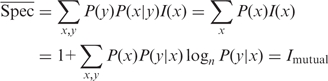
Figure 2.

Genomic distribution of cell specificity. Microarray data from 12 neuronal cell types and 11 789 genes in mouse and from 13 root tip cell types and 17 270 genes in Arabidopsis were used after filtered for uniquely mapping probes. The cell specificity index (Spec) was computed for each gene in each cell type. The cell type y* with highest Spec value was found for each gene. To assess significance for each dataset, we generated a shuffled dataset, by randomly permuting expression levels within each cell type across all genes. The distribution of [N_spec(y*), dSpec(y*)] over all genes is shown in shades of red (observed); the same distribution computed over a shuffled dataset is shown in shades of green (expected). Since the distributions overlap, each bin is colored according to the distribution whose value is larger, by a factor of two or more. Bins in which the observed and expected distributions do not differ by this criterion are colored dark blue; likewise in dark blue are bins which did not show a significant difference between the two distributions, based on a P-value < 0.001 criterion, computed using the Poisson distribution with the expected mean. Black bins are exclusively those for which both distributions are zero.

Estimation of Spec based on a small number of replicates

To test whether the bin-based estimator of Spec gave reliable results, given the small number of replicates available in each cell type (i.e. between two and four replicates per cell type), we constructed continuous probability distributions, P(x|y), using the plant microarray data. We calculated the mean and variance of the logarithm of expression levels, in each cell type. These were used to construct lognormal mock distributions of gene expression levels in each cell type. These distributions are merely for testing purposes, and do not necessarily reflect the true shapes of the distributions in each cell type. Using these mock distributions, we resampled the entire dataset, obtaining the same number of replicates in each cell type as existed in the real dataset. The constructed test dataset was used to obtain the bin-based estimate of Spec. The estimates were compared with the values obtained from the mock distributions by numerically integrating the lognormal distributions, according to the Spec formula given in Figure 1. The results are plotted in Supplementary Figure S5, and demonstrate that using three bins of expression provides a significant improvement over two bins. The improvement of using four bins over three bins is marginal, and we chose to use three bins for the entire analysis, since using fewer bins provides more statistical power when comparing the analysis with shuffled data. As the number of bins is increased beyond four, the correlation between estimated and true Spec values decreases, due to under-sampling of bins which results in spurious specificity values. Matlab and Perl code for Spec are available upon request.

Expression domains and cell-type networks (Spec networks)

The cell-type network was generated by identifying all genes whose expression domain size was 2 or 3 cell types (raw data, plant Supplementary Table S6, mouse Supplementary Table S7). By delineating the ‘fingers’ in Figure 2 that emanate from integral N_spec values along the dSpec = 0 axis, genes were identified for expression domains of size d = 2 or 3, according to the respective criteria 1.5 ≤ N_spec < 2.5 or 2.5 ≤ N_spec < 3.5. We also required a dSpec level <0.4, to avoid the false positive regions in Figure 2. Genes were then grouped into patterns based on their expression domain size d: the d cell types with the highest Spec values were labeled 1, and all other cell types were labeled 0. The number of genes g that comprised a significantly enriched pattern was identified by permuting gene expression values, generating N_spec values, and repeating the expression domain identification procedure. The observed value of g for each pattern was used to detect significantly enriched patterns, by requiring a value of g that was beyond the 95% percentile expected by chance assessed using the permuted data. This corresponded to having at least five genes display a pattern for the plant data and at least three genes for the mouse data; patterns satisfying this criterion were used as follows. The data was converted to an n-by-n matrix A, by summing the number of genes contributing to each pair of cell types occurring in each pattern. For example, for n = 5 cell types, if 10 genes shared pattern (1, 1, 0, 0, 1) a value of 10 was added to the entries A₁₂, A₁₅ and A₂₅, and so on for all significant patterns. To visualize major patterns, only edges with >100 genes for plants and >50 genes for mouse were drawn. The network was generated from the cell type by cell-type matrix using the Matlab biograph function with a hierarchal layout. Dendrograms in Figure 4 were generated using hierarchical clustering using Pearson correlation of overall gene expression values, and average linkage, after filtering out the 25% least varying genes in the dataset based on the variance of their average expression level across all cell types.

Figure 4.

Cell-type affinities in the Arabidopsis root and mouse brain. In Spec network representations, each edge represents a major pattern that linked the two cell types via a large number of genes (>100 genes in Arabidopsis; >50 genes in mouse) whose expression domains overlapped both cell types (see ‘Materials and Methods’ section). Dendrograms depict cell-type affinities using a similarity matrix of Pearson correlation of overall gene expression values. Gray edges in network represent cell types with high similarity in the tree where their ancestral node meets less than half the maximal distance. Black edges show cellular affinities that are distant in the similarity tree where their ancestral node meets at greater than half the maximal distance. Broken lines are longest distance relationships in the tree where their ancestral node is basal. (A) Phloem cells (red arrowheads) share a gene regulatory set (red circle) with adjoining pericycle cells (asterisks), showing a molecular domain of radial asymmetry (red square); radial asymmetry subfigure is reproduced from Figure 1b of (44); root subfigure was previously published in (3). QC cells, which support the growth of the primary meristem, share a strong affinity with lateral root meristem cells, which support the growth of lateral roots (blue circle). (B) Cells in the core of the limbic system of mouse, amygdala and hippocampus (blue circle), show strong affinities in the Spec network despite differences in the genetic background from which they came. In the similarity tree, some of the same cell types (e.g. amygdala cell samples) show distant relationships; brain subfigure is reproduced from http://stuff4educators.com/web_images/amygdala_hippocampus.jpg.

Gene ontology analysis

Lists of genes as described in the text were tested for over-representation of Gene ontology (GO) terms using Virtual Plant (13) (http://virtualplant.bio.nyu.edu) for Arabidopsis and GOrilla (14,15) for mouse. The background set was all genes in the Spec analysis (Supplementary Tables S1–S3), which excluded probes that mapped to two or more different transcripts. In each case, the hypergeometric distribution was used to assess overrepresentation.

Biomarker analysis

The data for hormone marker analysis included all treatments for each hormone without corresponding controls (raw data; Supplementary Table S8). Treatments for any given hormone were used as replicates regardless of whether they were generated in the same experimental series or lab in order to test performance in a metadata analysis. Spec values were generated as described above with each hormone treated as a separate category (Supplementary Table S9). GenePattern scores were generated using the Comparative Marker Selection tool with a ‘One versus All’ analysis for each hormone category using default settings (Supplementary Table S10). Genes were ranked by their overall ‘score’ statistic, as output from GenePattern. The documented auxin-responsive gene list was gathered from the literature and GO annotations (Supplementary Table S4).

Microarray datasets and probe-to-locus mapping

For the cell-type network analysis, microarray datasets for mouse neuronal cell types were obtained from (4) and Arabidopsis root tip cell types were obtained from (5,6,16). The publicly available mapping between microarray probes and genomic loci were used for each microarray (ftp://ftp.arabidopsis.org/home/tair/Microarrays/Affymetrix/). In most cases, Spec was computed for each locus based on a unique probe. In the rare cases when multiple probes mapped to a single genetic locus, the probe with the lowest N_spec value was used. All Affymetrix cell files were normalized with the MAS5 average intensity normalization method as implemented in the Affymetrix software. At a target intensity of 250, we determined empirically, using known markers, that a hybridization value of 50 represented a reliable expression signal. Thus, genes which did not express >50 were excluded from the analysis.

Hormone and white blood cell datasets

Published microarray datasets used for the hormone analysis were as follows (names of laboratories/datasets follow the conventions established in http://affymetrix.arabidopsis.info/narrays/help/usefulfiles.html). Abscisic Acid (ABA)—Helenius, Holman, RIKEN-GODA; Gibberellins (GA)—De Grauwe, Griffiths, Riken-Goda, RIKEN-LI; GA inhibitor—Riken-Goda; Auxin—Riken-Goda, Raghavan; Auxin inhibitor—Riken-Goda; Auxin transport inhibitor—Riken-Goda, Wenzel; Brassinosteroids—Riken-Goda; Brassinosteroid inhibitor—Riken-Goda; Cytokinin—Ljung, Riken-Goda, Sakakibara; Ethylene—Millenaar, Riken-Goda; Ethylene inhibitor—Riken-Goda; Jasmonate—Lewsey, Matthes, Riken-Goda; Salicylic Acid—Lewsey, Riken-Goda, St Clair. While all 13 types of hormones or inhibitors were used in the Spec analysis, Figure 7 displays the results for a subset of 10 selected hormones. For Human white blood cell profiles, all data and probe annotations were taken from Supplementary Data in (17). We used the quantile normalized, log₂ transformed data in the file HaemAtlasMKEBNormalizedIntensities.csv.proc, which was obtained from ArrayExpress (E-TABM-633), converting values back to their original scale (anti-log₂). We used a summary of well-documented CD marker by cell type expression (18) to infer a pattern of expression for 51 CD markers that we extracted from gene annotation files and manually annotated for presence/absence in seven cell types, filling a matrix with +1 (positive marker), −1 (negative marker), and 0 (unspecified marker) for each cell type. The megakaryocyte cell type was left out of the analysis because it was not specifically annotated in the summary table. A corresponding matrix of the N_spec and dSpec values was computed based on the mRNA expression profiles using each of the probes mapping to the known markers. The corresponding rows (CD markers) of the known expression table and the N_spec table were compared using Pearson correlation.

Figure 7.

Hormone-specific gene expression. Data from 250 experiments conducted in many different laboratories, in which specific hormone treatments were administered, was analyzed with hormone types taking the place of cell types in the analysis (see ‘Materials and Methods’ section). In each panel, labeled by the hormone type y, each gene was plotted as a single blue point at position [Spec(y), dSpec(y)]; red points represent the shuffled dataset. A brassinosteroid-responsive protein (brassinosteroid-6-oxidase 2, green circle) and an auxin-responsive protein (AT4G34770, purple circle) are highlighted for illustrative purposes. The auxin panel is shown in an enlarged view below, and the highly specific genes are labeled according to their genomic annotations. Several of the well-characterized auxin-responsive genes (IAA's) are seen to exhibit a high amount of noise across the multiple datasets used here; they are nevertheless among the most specifically expressed genes as measured by Spec. We note that each laboratory's control (null treatment) experiments were not used as part of this analysis as the meta-analysis, in effect, used all data for comparisons. Spec and dSpec values were computed using three expression level bins.

RESULTS

The specificity measure

We begin by addressing the problem of cell-type specificity abstractly, and then tailor our approach to various kinds of data. We assume that a gene is characterized by a distribution of its expression level x, in each cell type y (out of n different cell types) and label this distribution P(x|y). The question of how to measure P(x|y) in practice is addressed in ‘Materials and Methods’ section. For now, let us imagine that P(x|y) is known to us and to a colleague, and suppose we play the following game. In a given cell type y, we make a single measurement of the gene expression level. We present this measurement x to our colleague, but we do not reveal the cell identity y. We would like to know, when presenting the measurement from cell type y, on average how much information regarding the cell type have we given to our colleague. For example, if there are many cell types, and a gene is expressed only in a single cell type y₀, a measurement of the gene's level in y₀ will be highly informative for our colleague, while a measurement from a different cell type will be uninformative. The measure Spec(y), defined below, quantifies this notion precisely.

To define Spec(y), we first invert the distribution using Bayes’ rule (19), to obtain P(y|x), i.e. the probability that a cell is of type y given that the gene's level is observed to be x (Figure 1b),

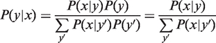where we assume that our colleague has no a priori knowledge about cell types, i.e. P(y) = 1/n, though one can easily incorporate a non-uniform prior. We then ask how informative is expression level x regarding the cell type. Figure 1b presents an idealized example, where a single gene has been measured in six cell types, and expression levels are binned into three possible states. Measurements in the ‘low’ range are uninformative, since five of the cell types are found to exhibit such levels. Measurements in the ‘medium’ and ‘high’ ranges are partially informative, since only two cell types have these levels, with the high range being more informative than the medium range. No measurement is maximally informative, since some ambiguity about the cell type remains no matter which level is measured.

We compute the ‘information’ (20), I(x), of gene expression level x:

By using the base of the logarithm to be n (the number of cell types), possible values of I(x) lie in the range from 0 (uninformative) to 1 (maximally informative). To obtain the ‘specificity value’, Spec(y), we average the values of I(x) over the distribution P(x|y) of gene expression levels for each cell type:

Intuitively, Spec(y) indicates the average amount of information about the cell's identity that is provided by a measurement of the gene's expression level in cell type y. In the Figure 1b example, Spec(y) is found to be highest in cell type C, intermediate in cell types E and B, and low in the other three types; I(x) indicates that this gene is not maximally informative at any level, and therefore Spec is not maximally high in any cell type.

We also define the quantity N_spec(y) ≡ n^1−Spec(y) which is the effective number of cell types (not necessarily integral) specified by the gene's expression level in cell type y. This is equivalent to the effective number of states specified by a probability distribution using the exponential of the distribution's entropy (20). To summarize specificity of a gene, we will omit y, writing N_spec to indicate the maximal value of N_spec(y) over all cell types. A maximally specific gene has N_spec = 1, while a minimally specific gene has an N_spec = n, the number of cell types.

Spec is related to a well-known information-theoretic measure, the mutual information (20), I_mutual, which in our above formulation is given by

where P(x,y) = P(x)P(y|x) is the joint probability of x and y. If we average the values of Spec(y) over the cell type distribution P(y), we find

Thus, the average value of Spec(y) over all cell types gives the mutual information between cell type and gene expression level. Mutual information provides an overall measure of the specificity of a gene, but is not a cell-type specific measure and can give counter-intuitive results for highly specific genes. To see this, we return to the example of the gene that is expressed only in cell type y₀. It is clear that the larger the number of cell types n, the lower the mutual information between this gene's expression level and the cell type; Spec(y₀), on the other hand, will be 1 regardless of the number of cell types. Spec(y) is a more detailed and sensitive quantity than mutual information.

Effect of noise on specificity (dSpec)

Depending on experimental approach, different types of noise exist in each data set. Typical sources of noise include (i) technical noise, due to the experimental preparation and measurement technique, (ii) sample composition noise, due to replicate samples, which may differ depending on how they were collected, and (iii) single-cell biological noise, due to inherently random processes within single cells. For the datasets we examine, which consist of large pools of cells, the main sources of noise are (i) and (ii). Our approach does not attempt to disentangle these different sources, and their sum total effect results in the distribution of expression levels P(x|y). We now consider how specificity is affected in genes with different levels of noise.

Consider Scenario A (low noise) in which two different genes are measured in 12 cell types (Supplementary Figure S1). Gene 1 is expressed at high level in two cell types, and at low level in the 10 other cell types. This gene has a Spec value of 0.72 in the two high-expression cell types, with a corresponding N_spec value of 2. Gene 2 is expressed at high level in three cell types, and at low levels in nine other cell types. Accordingly, in the three high-expression cell types, its Spec value is 0.56 with an N_spec value of 3. With low noise in each case, high Spec values identify the cell types that share a specific expression level, i.e. the gene's ‘expression domain’. However, in a separate Scenario B (high noise), expression levels in the first gene are noisy at low levels and its Spec value is thus significantly <0.72, with a value of 0.52 and an N_spec value of 3.3. Adding noise to a gene with an expression domain of two cell types leads to Spec values resembling a gene with an expression domain of three cell types.

To distinguish the lack of specificity due to larger expression domains from lack of specificity due to noise we generalize the Spec measure. We analyze the case of presenting our colleague with two independent measurements, x₁ and x₂, from the same cell type. In Scenario A above, two measurements provide no more information than one measurement, since low noise implies that both measurements will record similar values. In Scenario B, however, the two measurements are likely to differ in cell types in which expression is noisy, and to be identical in cell types with less noise. This results in excess information of two measurements versus one, which our colleague can use to distinguish among cell types. The lower the excess information, the more difficult it is to distinguish among cell types within the gene's expression domain, and the more specific of the domain as a unit is the gene. The measure dSpec(y), below, quantifies this notion.

To define dSpec, we first use Bayes’ rule to obtain the distribution of y conditional on the two measurements, x₁ and x₂:

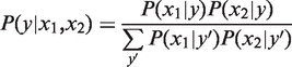The information is likewise generalized as I(x₁,x₂) = , and we define the quantity Spec₂(y), which is the amount of information expected based on the two measurements in cell type y:

We then define dSpec as the relative excess information:

In Scenario B (Supplementary Figure S1), dSpec detects that the gene's specificity is affected by noise, with dSpec values of 0.21 in cell types 2 and 4, and dSpec values of 0.91 in types 5 and 11. In Scenario C, however, expression in three cell types is noisy, but with very similar noise profiles in all three types. Although noise is present, expression is nevertheless specific of three cell types (2, 4 and 7), resulting in an N_spec value of 3 (Spec = 0.56), and a dSpec value of 0. Thus, noise does not necessarily reduce specificity, and dSpec effectively distinguishes and quantifies the effect of noise on specificity.

It is natural to consider further generalization, in which m independent measurements from cell type y are presented to our colleague, and a more general quantity Spec_m(y) is computed, for m > 2. Clearly, the larger the number of measurements, the finer the differences in gene expression profiles P(x|y) that can be distinguished. While it is straightforward to work out the amount of information obtained in the limit of large m, this limit is not useful for our purposes, because it is dominated by the process of distinguishing among the most similar cell types, typically those belonging to the gene's expression domain. For example, for a gene expressed only in cell type y₀, any noise in its expression level reduces its specificity in a way that is detected by dSpec(y₀) and thus attributed to noise rather than to having a larger expression domain. If instead of m = 2, we use a much larger number of measurements, we will find that Spec_m(y₀) ≈ 1, i.e. noise no longer reduces specificity, and for large enough m we may even have Spec_m(y) ≈ 1 in many other cell types y ≠ y₀. The value m = 2 is thus appropriate for assessing the impact of noise on expression domains. One can think of dSpec as measuring the first-order or principal effect of noise on domains, whereas larger values of m can detect higher order or secondary effects.

Expression domains and the genomic distribution of specificity

We applied Spec to quantify transcriptome structure over a broad taxonomic range, using two datasets that profiled a large number of cell types within a specific organ, and calculated Spec for each gene in each cell type. The first dataset included profiles of 13 morphologically identifiable cell types in the Arabidopsis root (5,6,16), obtained by Fluorescence Activated Cell Sorting (FACS) of cell-type specific marker lines and profiled on the ATH1 microarray (Affymetrix). The second dataset consisted of 12 different types of mouse neurons (4), which were manually sorted, pooled, and applied to the MOE430A microarray (Affymetrix).

We define the gene's expression domain as the set of cell types for which the gene's expression level is most informative (see ‘Materials and Methods’ section). N_spec measures the size of the gene's expression domain, i.e. the effective number of cell types which the gene specifies in its expression pattern. For example, the gene in Scenario B (Supplementary Figure S1) has an N_spec value of 3.3, indicating that the gene is effectively informative of between three and four cell types, without forming a perfect pattern. The value of dSpec ≈ 0.2 in the two highest Spec cell types (types 2 and 4) indicates the presence of noise in other cell types (types 5 and 11) which reduces specificity. Alternatively, for genes that display perfect patterns, dSpec values will be 0, and N_spec values will be integral.

The global distribution of specificity (Figure 2) displays the expression domain sizes and their noise levels across the genome. The bright spot at N_spec = 1 indicates the existence of a large set of ‘private transcripts’, genes whose expression domain is exclusive to single cell types. One striking feature of the data is that a majority of genes have larger expression domains, i.e. they are not specific to a single cell type but are rather shared by at least two to five other cell types (Figure 2). These expression domains appear as bright fingers along the left side of the Figure 2 in the low-noise part of the distribution, which demonstrates that these are essentially clean patterns, with a small amount of gene expression noise. The shuffling analysis described in the caption to Figure 2 shows that these patterns are significant and indeed more prevalent than single cell-type specificity. While previous studies of genomic datasets identified particular expression patterns using clustering methods (5,6), the Spec-based analysis shows rigorously that the vast majority of the transcriptome exhibits multi cell-type expression domains, a feature that appears to be shared across the wide taxonomic distance between plants and mice.

Cell types have a large component of neighbor- and tissue-shared programs

The Spec measure provides a way to systematically study cell-type specificity across the genome by examining genes with increasingly larger expression domains, as shown in Figure 3 for two different cell types. The different N_spec intervals identify genes with different size expression domains that overlap a given cell type. The number of unique and shared transcripts in each cell type are shown in Supplementary Figure S3. We used the Spec measure to map expression domains onto specific cells using a network representation (Spec network), shown in Figure 4, in which each edge denotes a sufficiently large number of genes whose domains include the two cell types (see ‘Materials and Methods’ section). For comparison, we also generated a similarity tree based on averages of the normalized data.

Figure 3.

Expression domains of genes across cell types. Data is shown for Arabidopsis phloem companion cells and for the mouse G30-amygdala cells. For each cell type, three plots are given, representing domains of size 2, 3 and 4. For domain size D, we included all genes whose D lowest N_spec(y) values were <D + 0.5, and which had all other N_spec(y) values greater than D + 1. We required that the D cell types with lowest N_spec(y) values include the given cell type (phloem companion or G30-amygdala). Both Spec and raw expression data are shown. Genes are sorted according to the order (left to right) of the D cell types in the gene's domain, and further sorted according to the Spec value of the left-most cell type in the domain. Additionally, genes exhibiting low expression in the cell type of maximal Spec are sorted to the bottom of the plot, allowing these genes to be easily noticed visually.

The analysis reveals the transcriptional programs that are shared by neighboring tissues. For example, in plants, the Spec network reveals a strong transcriptional link between phloem cells and a subset of pericycle cells that neighbor them in the central cylinder (Figure 4); this connection is not apparent in the similarity tree, yet is supported by both the spatial proximity of the cell types and genetic perturbations that simultaneously affect both phloem and pericycle identity adjacent to the phloem (21). In mouse, the similarity tree is unable to establish the affinity between amygdala cells collected from adjacent layers in the brain, possibly because they were harvested from mice of different genetic backgrounds (Figure 4). However, the Spec network reveals a large set of transcripts shared between them.

Spatially separated cell types can be linked by shared transcriptional programs

We also find that transcripts can be shared by cell types that are separated spatially across organs. For example, quiescent center (QC), which supports the growth of stem cells in the root niche (22,23), was connected largely to adjacent cell types, as in the similarity tree (Figure 4). However, the QC also shared one major edge with progenitor cells of the lateral root meristem, a distant cell type that is nonetheless also associated with root growth (24,25) (Figure 4). A few critical regulators for meristem function, such as PLETHORA2 (26), are known to be specifically expressed in both stem cell populations. However, the Spec network identifies a more global functional link between these cell types. For example, genes that share a high Spec in QC and lateral root meristem were over-represented in plastid formation (plastid fission, P < 10⁻²; Supplementary Table S1). In support of this functional link, mutants in plastid formation have been shown to have stem cell-specific defects in plant roots (27). Once again, the specific connection between the two cell types was not obvious from the similarity tree or common clustering routines (Figure 4 and Supplementary Figure S2). In the mouse brain, the Spec network linked together four cell types or subtypes within a part of the classically defined limbic system, the hippocampus and amygdala, for which functional and synaptic ties have been noted by recent morphological and molecular genetic studies (28). Interestingly, in both organisms, we found that certain functional categories of genes tended to have similar domain sizes even if they were expressed in different cell types (Supplementary Tables S2 and S3).

Using Spec for biomarker identification

As shown in Figures 2 and 3, high Spec values identify highly specific gene expression patterns, with dSpec assessing the noisiness of the pattern. These metrics should also be useful for biomarker discovery, as is frequently sought in cancer diagnostics (29,30). We tested this possibility by using two case studies in which large datasets and known markers for specific conditions were available.

The first dataset consisted of expression profiles of eight different white blood cell types from seven healthy subjects analyzed on the Illumina BeadChip platform (17). This dataset provided an opportunity to test Spec against the large and well-documented set of cluster of differentiation (CD) markers, whose specificity varies expression in one to many of the cell types (31). We reasoned that, in a large-scale validation using markers selected to reflect on–off states, mRNA expression patterns should broadly reflect the protein levels measured by cell-surface markers. In addition, the samples in this dataset represented individuals, permitting us to use dSpec to assess robustness of expression in replicate cell types, a measure of cell-type plasticity among individuals that has clinical relevance.

We coded known positive and negative markers for each cell type into a table of +1 and −1 values, respectively, and correlated the table to N_spec values generated from the empirical data in the expression study (see ‘Materials and Methods’ section, Figure 5). The highest correlation was among the narrowly expressed markers, those present in one, two or three cell types (average r = 0.72, 0.85, 0.63 respectively), with 12 out of these 26 markers having correlation 0.97 or higher. Correlation drops off rapidly for markers that were broadly expressed (i.e. in four, five, six, or seven cell types). The results showed that Spec is highly effective in identifying known markers, including markers with more complex patterns of expression in several cell types and absence in others.

Figure 5.

Validation of Spec against well-documented white blood cell markers. (left panels) The heatmap depicts the known expression profile (18) of 51 CD markers in the seven cell types tested (see ‘Materials and Methods’ section). Positive markers (blue), negative markers (white) and unspecified markers (gray) are indicated. From top to bottom, groups of rows show markers expressed in an increasing number of cell types, from one cell type (top rows) to seven cell types (bottom rows). Three markers that had two probes each are listed twice (CD163, probes ILMN_1722622/ILMN_1733270; CD74, probes ILMN_1736567/ILMN_1761464; and CD86, probes ILMN_1651349/ILMN_1714602). (Middle panels) The heatmap shows the N_spec values for the makers calculated from expression data (17) (‘Materials and Methods’ section). The Pearson correlations, r, between marker values (−1, 0, 1) and N_spec values are listed, and indicate a high level of concordance for markers expressed in up to three cell types between known cell-surface expression patterns (left panels) and N_spec values calculated from expression profiles (middle panels). A heatmap of dSpec values (right panels) for each gene in each cell type shows the level and cell-type distribution of noise for each gene, indicating a trend of decreasing robustness for more widely expressed genes. Arrows indicate the two examples that are discussed in the text.

The analysis also illustrates the potential of dSpec to assess robustness for a given marker at high resolution. For example, CD14 is specific to monocytes and granulocytes, as known from its use as a cell surface marker and predicted by its N_spec values. The marker's dSpec values are relatively low in its negative cell types but moderately high in one of its positive cell types (granulocytes). Such a noise profile suggests that the marker is prone to false negatives but not false positives, a case where noise may be tolerable when multiple markers are used. The marker exhibits a reliable-when-present plasticity such that when it is present, it identifies granulocytes with high confidence. However, not all individuals express the marker in granulocytes. On the other hand, CD123 is highly specific to granulocytes, where it exhibits low noise (low dSpec), while its dSpec is high in all cell types other than granulocytes. Such a profile suggests that CD123 is highly informative of granulocytes but its high noise in the other cell types, where its expression levels vary among individuals, makes it potentially prone to false positives. The marker exhibits a plasticity in which virtually all individuals express CD123 at a specific level in granulocytes yet individuals show variable expression levels in almost all other cell types.

Overall, we find that mRNA expression plasticity as measured by dSpec increases for markers transcribed in an increasingly larger number of cell types (Figure 5). Such a trend, as detected by Spec's quantification of specificity and noise, has practical implications. For example, if a negative marker is needed to sort against a cell population, that population will be more reliably identified by a set of narrow markers than a single broad marker (assuming that mRNA noise levels reflect protein-level noise in the case of cell-surface markers). Thus, Spec and dSpec provide a way to assess marker specificity and plasticity, respectively; in particular, dSpec can detect whether specificity is reduced due to noise inside or outside of the gene's expression domain.

In the second dataset, we used a large compendium of hormone treatment microarray data from many different labs (http://affymetrix.arabidopsis.info/narrays/experimentbrowse.pl). The use of this dataset permitted us to benchmark Spec against one other common biomarker discovery tool using a large set of genes known to respond in one condition, auxin treatment (Supplementary Table S4). We asked whether Spec could make use of the information in a meta-analysis consisting of 250 samples collected in 14 different labs.

A number of quantitative approaches have been applied to finding biomarkers, including support vector machines, neural networks and others (32–36). We tested Spec against one highly cited and well-documented tool, GenePattern (1,37), which bases pattern discovery on a t-test with calculated false discovery rates. The test set contained treated samples for 13 hormones or hormone inhibitors, with no controls included (since the 12 other classes served as background or non-target classes). In each case, we tested for auxin-specific responses, examining the top ranked genes for each algorithm to compare performance of the two approaches (Figure 6A). Spec was notably precise at stringent levels. Among the top 20 ranked markers identified by each method, Spec identified 10 known markers while GenePattern identified two (Supplementary Table S5). Both methods capture highly specific markers with consistently high expression in the target class and low expression in the non-target class, although we note this is a relatively small percentage of the known markers. At low stringency levels (>250 highest ranked), GenePattern was able to find more markers than Spec (24 versus 15 in the top 500 ranked) but precision at these stringency levels was very low.

Figure 6.

Biomarker discovery performance for Spec and GenePattern. (A) The graph shows the precision (true positive/total positive cases) of each biomarker approach in identifying 221 documented auxin-responsive markers among profiles of 17 285 genes in a series of 13 different hormone treatments. The identity of markers was obtained from literature, not from the data itself. For every gene, each method generates a marker score for each hormone [e.g. Spec(auxin)] and genes were ranked from highest to lowest score in the auxin category, using only those genes in which the auxin score was highest among all hormones. To obtain the precision of each method at a given ranked gene list size (i.e. top 20 genes, top 40 genes, etc), the number of true hits in the list were tallied and divided by the list size. (B) Within the top 500 ranking genes for each approach, graphs show the expression patterns of the highest-ranking documented auxin markers discovered by one method but not the other. The graph shows expression in all the experiments used by each method to evaluate the markers, with the auxin experiments highlighted nearest to the origin.

Another unique property of Spec as a biomarker discovery tool is its ability to identify complex markers that are informative of more than one condition, as demonstrated in Figures 2–4. For example, the documented auxin-responsive transcript (AT4G34770) has a relatively high Spec for auxin and for ethylene (Figure 7, purple circle). Interestingly, its noise within the auxin data is relatively high and it is not likely to be identified as an auxin marker using traditional statistical methods. Similarly, brassinosteroid-6-oxidase 2, which is involved in brassinosteroid biosynthesis, is induced by both brassinosteroid and GA inhibitors, the latter of which exhibits high variance within treatments and would likely have been missed by statistical methods (Figure 7, green circle). Thus, analogous to its potential in linking the function of cells, the quantification of specificity provides a way of linking common responses to diverse conditions.

DISCUSSION

We have described a rigorous approach that uses information theory to formalize the concept of specificity in gene expression and to quantify cell identity in the presence of noise. More generally, the approach is applicable when biological measurements x (e.g. mRNA expression levels, protein abundances, epigenetic modifications, etc.) are mapped onto a biological organization y (e.g. cell types, spatial structure, treatments, disease states, etc.)—and the mapping is given by a probability distribution P(x|y). Information-based approaches in developmental biology have previously focused on transmission of information within developmental regulatory circuits (38,39). Our application of Spec here addresses a novel question, namely how much information does a gene's expression level provide about a cell's identity. As such, Spec provides both a unifying conceptual framework and a measurement tool in the study of cell identity, and with it the ability to quantify on a genome-wide scale this central concept of developmental biology.

The formulation presented here makes it possible to distinguish noise that detracts from information on cell-type specificity from noise which does not, by using the measure dSpec. This unique feature of the method is generally missing in purely statistical approaches, such as analysis of variance or measures based on the t-test. The ability to cope with various sources of noise in data reveals critical connections between cell types, as well as unique and promising classes of biomarkers. When technical replicate data are used, dSpec detects cases when variability among samples detracts from specificity. When samples from different individuals are used, dSpec provides a measure of transcriptional plasticity for each gene in each cell type. In its biomarker applications, dSpec therefore makes it possible to pinpoint cell types in which plasticity is most likely to result in false positives, and to identify markers that are more likely to be reliable for a given target class.

The Spec analysis provides a new tool to explore the mosaic character of gene expression in a multicellular organism. In the plant and animal examples examined, most specifically expressed genes have expression domains containing between two and five cell types (Figures 2 and 3), with shared gene expression describing potentially novel mechanistic links between cell types. The quantification of specificity and noise also reveals the limits of complex pattern detection, i.e. patterns consisting of more than five or six cell-type domains could not be precisely delineated given the noise in the data (Figure 2). The genomic signature of cell-type specificity, i.e. the bright fingers in Figure 2, is notably absent in the hormone dataset (Supplementary Figure S4), demonstrating that the signature is neither a generic feature of microarray data nor an artifact of the approach. In addition, cell identity has a component of specifically absent gene activity, i.e. transcripts expressed in all but one or a few cell types (Figure 3).

As a quantitative measure of specificity, Spec also opens possibilities for phylogenetic studies to map changes in cellular complexity during evolution (3,40–43). The next generation of genomics may allow entire transcriptomes to be routinely measured in individual cells, rather than in pooled samples. It will be particularly interesting to see individual differences among single cells using Spec, and to determine which parts of the overall genomic distribution of specificity, shown in Figure 2, are maintained at the single cell level, and which new aspects of specificity are revealed. By virtue of having information theory at its basis, Spec provides a consistent framework for comparing our current measurements of specificity, with those enabled by future technological advances in genomics.

Spec's significantly higher precision in biomarker identification is due to its handling of noise, which permits markers to exhibit significant variability within the target class (Figure 6B). This is arguably a common property of many otherwise reliable markers, which are specific to the target condition but variable in their response. On the other hand, most of the markers missed by Spec and identified by GenePattern showed high levels of noise in the non-target set but a consistently higher level of expression in the target set (Figure 6B). Such markers could be prone to false positive tests and may pose a problem for diagnostics.

We have described the formulation and application of Spec, an information-theoretic specificity measure that allows a rigorous quantification of cell identity in biological systems. Using information theory as the basis for measuring specificity allows both ease of interpretation and flexibility of application. Moreover, it necessitates the incorporation of noise as an integral component of the specificity measure. As we have shown, this critical facet of our approach allows features of genomic data that are typically ignored or discarded due to variability to be meaningfully analyzed and quantified. Without our explicit accounting of noise, many of the structures revealed in the datasets we have analyzed (transcription patterns, biomarkers, cell-type connections) would have been entirely missed. The flexibility and generality of the method, combined with its rigorous treatment of noise, provide a powerful approach for quantitative analysis of specificity in biology.

SUPPLEMENTARY DATA

Supplementary Data are available at NAR Online.

FUNDING

Burroughs Wellcome Career Award at the Scientific Interface (to E.K.); National Institutes of Health (grant R01 GM078279 to K.D.B.). Funding for open access charge: Burroughs Wellcome Fund and National Institutes of Health.

Conflict of interest statement. None declared.

REFERENCES

- 1.Gould J, Getz G, Monti S, Reich M, Mesirov JP. Comparative gene marker selection suite. Bioinformatics. 2006;22:1924–1925. doi: 10.1093/bioinformatics/btl196. [DOI] [PubMed] [Google Scholar]
- 2.Espinosa-Soto C, Wagner A. Specialization can drive the evolution of modularity. PLoS Comput. Biol. 2010;6:e1000719. doi: 10.1371/journal.pcbi.1000719. [DOI] [PMC free article] [PubMed] [Google Scholar]
- 3.Arendt D. The evolution of cell types in animals: emerging principles from molecular studies. Nat. Rev. Genet. 2008;9:868–882. doi: 10.1038/nrg2416. [DOI] [PubMed] [Google Scholar]
- 4.Sugino K, Hempel CM, Miller MN, Hattox AM, Shapiro P, Wu C, Huang ZJ, Nelson SB. Molecular taxonomy of major neuronal classes in the adult mouse forebrain. Nat. Neurosci. 2006;9:99–107. doi: 10.1038/nn1618. [DOI] [PubMed] [Google Scholar]
- 5.Birnbaum K, Shasha DE, Wang JY, Jung JW, Lambert GM, Galbraith DW, Benfey PN. A gene expression map of the Arabidopsis root. Science. 2003;302:1956–1960. doi: 10.1126/science.1090022. [DOI] [PubMed] [Google Scholar]
- 6.Brady SM, Orlando DA, Lee JY, Wang JY, Koch J, Dinneny JR, Mace D, Ohler U, Benfey PN. A high-resolution root spatiotemporal map reveals dominant expression patterns. Science. 2007;318:801–806. doi: 10.1126/science.1146265. [DOI] [PubMed] [Google Scholar]
- 7.Shen-Orr SS, Tibshirani R, Khatri P, Bodian DL, Staedtler F, Perry NM, Hastie T, Sarwal MM, Davis MM, Butte AJ. Cell type-specific gene expression differences in complex tissues. Nat. Methods. 2010;7:287–289. doi: 10.1038/nmeth.1439. [DOI] [PMC free article] [PubMed] [Google Scholar]
- 8.Chambers SM, Boles NC, Lin KK, Tierney MP, Bowman TV, Bradfute SB, Chen AJ, Merchant AA, Sirin O, Weksberg DC, et al. Hematopoietic fingerprints: an expression database of stem cells and their progeny. Cell Stem Cell. 2007;1:578–591. doi: 10.1016/j.stem.2007.10.003. [DOI] [PMC free article] [PubMed] [Google Scholar]
- 9.Acar M, Becskei A, van Oudenaarden A. Enhancement of cellular memory by reducing stochastic transitions. Nature. 2005;435:228–232. doi: 10.1038/nature03524. [DOI] [PubMed] [Google Scholar]
- 10.Raj A, van Oudenaarden A. Single-molecule approaches to stochastic gene expression. Annu. Rev. Biophys. 2009;38:255–270. doi: 10.1146/annurev.biophys.37.032807.125928. [DOI] [PMC free article] [PubMed] [Google Scholar]
- 11.Raj A, van Oudenaarden A. Nature, nurture, or chance: stochastic gene expression and its consequences. Cell. 2008;135:216–226. doi: 10.1016/j.cell.2008.09.050. [DOI] [PMC free article] [PubMed] [Google Scholar]
- 12.Kurimoto K, Yabuta Y, Ohinata Y, Saitou M. Global single-cell cDNA amplification to provide a template for representative high-density oligonucleotide microarray analysis. Nat. Protoc. 2007;2:739–752. doi: 10.1038/nprot.2007.79. [DOI] [PubMed] [Google Scholar]
- 13.Katari M, Nowicki S, Aceituno F, Nero D, Kelfer J, Thompson L, Cabello J, Davidson R, Goldberg A, Shasha D, et al. VirtualPlant: a software platform to support systems biology research. Plant Physiol. 2010;152:500–515. doi: 10.1104/pp.109.147025. [DOI] [PMC free article] [PubMed] [Google Scholar]
- 14.Eden E, Lipson D, Yogev S, Yakhini Z. Discovering motifs in ranked lists of DNA sequences. PLoS Comput. Biol. 2007;3:e39. doi: 10.1371/journal.pcbi.0030039. [DOI] [PMC free article] [PubMed] [Google Scholar]
- 15.Eden E, Navon R, Steinfeld I, Lipson D, Yakhini Z. GOrilla: a tool for discovery and visualization of enriched GO terms in ranked gene lists. BMC Bioinformatics. 2009;10:48. doi: 10.1186/1471-2105-10-48. [DOI] [PMC free article] [PubMed] [Google Scholar]
- 16.Nawy T, Lee J, Colinas J, Wang J, Thongrod S, Malamy J, Birnbaum K, Benfey P. Transcriptional profile of the Arabidopsis root quiescent center. Plant Cell. 2005;17:1908–1925. doi: 10.1105/tpc.105.031724. [DOI] [PMC free article] [PubMed] [Google Scholar]
- 17.Watkins NA, Gusnanto A, de Bono B, De S, Miranda-Saavedra D, Hardie DL, Angenent WG, Attwood AP, Ellis PD, Erber W, et al. A HaemAtlas: characterizing gene expression in differentiated human blood cells. Blood. 2009;113:e1–e9. doi: 10.1182/blood-2008-06-162958. [DOI] [PMC free article] [PubMed] [Google Scholar]
- 18. CD Marker Handbook Human CD Markers. (2010) BD Biosciences, San Jose, CA.
- 19.Casella G, Berger R. Statistical Inference. Pacific Grove, CA: Thomson Learning; 2002. [Google Scholar]
- 20.Cover T, Thomas J. Elements of Information Theory. New York: John Wiley & Sons, Inc; 1991. [Google Scholar]
- 21.Parizot B, Laplaze L, Ricaud L, Boucheron-Dubuisson E, Bayle V, Bonke M, De Smet I, Poethig SR, Helariutta Y, Haseloff J, et al. Diarch symmetry of the vascular bundle in Arabidopsis root encompasses the pericycle and is reflected in distich lateral root initiation. Plant Physiol. 2008;146:140–148. doi: 10.1104/pp.107.107870. [DOI] [PMC free article] [PubMed] [Google Scholar]
- 22.van den Berg C, Willemsen V, Hendriks G, Weisbeek P, Scheres B. Short-range control of cell differentiation in the Arabidopsis root meristem. Nature. 1997;390:287–289. doi: 10.1038/36856. [DOI] [PubMed] [Google Scholar]
- 23.Matsuzaki Y, Ogawa-Ohnishi M, Mori A, Matsubayashi Y. Secreted peptide signals required for maintenance of root stem cell niche in Arabidopsis. Science. 2010;329:1065–1067. doi: 10.1126/science.1191132. [DOI] [PubMed] [Google Scholar]
- 24.Malamy JE, Benfey PN. Organization and cell differentiation in lateral roots of Arabidopsis thaliana. Development. 1997;124:33–44. doi: 10.1242/dev.124.1.33. [DOI] [PubMed] [Google Scholar]
- 25.De Smet I, Vassileva V, De Rybel B, Levesque MP, Grunewald W, Van Damme D, Van Noorden G, Naudts M, Van Isterdael G, De Clercq R, et al. Receptor-like kinase ACR4 restricts formative cell divisions in the Arabidopsis root. Science. 2008;322:594–597. doi: 10.1126/science.1160158. [DOI] [PubMed] [Google Scholar]
- 26.Aida M, Beis D, Heidstra R, Willemsen V, Blilou I, Galinha C, Nussaume L, Noh Y-S, Amasino R, Scheres B. The plethora genes mediate patterning of the arabidopsis root stem cell niche. Cell. 2004;119:109–120. doi: 10.1016/j.cell.2004.09.018. [DOI] [PubMed] [Google Scholar]
- 27.Benitez-Alfonso Y, Cilia M, San Roman A, Thomas C, Maule A, Hearn S, Jackson D. Control of Arabidopsis meristem development by thioredoxin-dependent regulation of intercellular transport. Proc. Natl Acad. Sci. USA. 2009;106:3615–3620. doi: 10.1073/pnas.0808717106. [DOI] [PMC free article] [PubMed] [Google Scholar]
- 28.Fanselow MS, Dong HW. Are the dorsal and ventral hippocampus functionally distinct structures? Neuron. 2010;65:7–19. doi: 10.1016/j.neuron.2009.11.031. [DOI] [PMC free article] [PubMed] [Google Scholar]
- 29.Golub TR, Slonim DK, Tamayo P, Huard C, Gaasenbeek M, Mesirov JP, Coller H, Loh ML, Downing JR, Caligiuri MA, et al. Molecular classification of cancer: class discovery and class prediction by gene expression monitoring. Science. 1999;286:531–537. doi: 10.1126/science.286.5439.531. [DOI] [PubMed] [Google Scholar]
- 30.Alizadeh AA, Eisen MB, Davis RE, Ma C, Lossos IS, Rosenwald A, Boldrick JC, Sabet H, Tran T, Yu X, et al. Distinct types of diffuse large B-cell lymphoma identified by gene expression profiling. Nature. 2000;403:503–511. doi: 10.1038/35000501. [DOI] [PubMed] [Google Scholar]
- 31.Diaz-Ramos MC, Engel P, Bastos R. Towards a comprehensive human cell-surface immunome database. Immunol Lett. 2011;134:183–187. doi: 10.1016/j.imlet.2010.09.016. [DOI] [PubMed] [Google Scholar]
- 32.Abeel T, Helleputte T, Van de Peer Y, Dupont P, Saeys Y. Robust biomarker identification for cancer diagnosis with ensemble feature selection methods. Bioinformatics. 2010;26:392–398. doi: 10.1093/bioinformatics/btp630. [DOI] [PubMed] [Google Scholar]
- 33.Brunet JP, Tamayo P, Golub TR, Mesirov JP. Metagenes and molecular pattern discovery using matrix factorization. Proc. Natl Acad. Sci. USA. 2004;101:4164–4169. doi: 10.1073/pnas.0308531101. [DOI] [PMC free article] [PubMed] [Google Scholar]
- 34.Yeang CH, Ramaswamy S, Tamayo P, Mukherjee S, Rifkin RM, Angelo M, Reich M, Lander E, Mesirov J, Golub T. Molecular classification of multiple tumor types. Bioinformatics. 2001;17(Suppl. 1):S316–S322. doi: 10.1093/bioinformatics/17.suppl_1.s316. [DOI] [PubMed] [Google Scholar]
- 35.Bicciato S, Luchini A, Di Bello C. Marker identification and classification of cancer types using gene expression data and SIMCA. Methods Inf. Med. 2004;43:4–8. [PubMed] [Google Scholar]
- 36.Bicciato S, Pandin M, Didone G, Di Bello C. Pattern identification and classification in gene expression data using an autoassociative neural network model. Biotechnol Bioeng. 2003;81:594–606. doi: 10.1002/bit.10505. [DOI] [PubMed] [Google Scholar]
- 37.Reich M, Liefeld T, Gould J, Lerner J, Tamayo P, Mesirov JP. GenePattern 2.0. Nat. Genet. 2006;38:500–501. doi: 10.1038/ng0506-500. [DOI] [PubMed] [Google Scholar]
- 38.Gregor T, Tank D, Wieschaus E, Bialek W. Probing the limit to positional information. Cell. 2007;2007:153–164. doi: 10.1016/j.cell.2007.05.025. [DOI] [PMC free article] [PubMed] [Google Scholar]
- 39.Tkacik G, Callan CJ, Bialek W. Information flow and optimization in transcriptional regulation. Proc. Natl Acad. Sci. USA. 2008;105:12265–12270. doi: 10.1073/pnas.0806077105. [DOI] [PMC free article] [PubMed] [Google Scholar]
- 40.Valentine JW, Collins AG, Meyer CP. Morphological complexity increase in metazoans. Paleobiology. 1994;20:131–142. [Google Scholar]
- 41.Hinegardener R, Engelberg J. Biological complexity. J. Theor. Biol. 1983;104:7–20. [Google Scholar]
- 42.McShea DW. Perspective: metazoan complexity and evolution: is there a trend? Evol. Int. J. Org. Evol. 1996;50:447–492. doi: 10.1111/j.1558-5646.1996.tb03861.x. [DOI] [PubMed] [Google Scholar]
- 43.Carroll SB. Chance and necessity: the evolution of morphological complexity and diversity. Nature. 2001;409:1102–1109. doi: 10.1038/35059227. [DOI] [PubMed] [Google Scholar]
- 44.Mahonen A, Bishopp A, Higuchi M, Nieminen K, Kinoshita K, Tormakangas K, Ikeda Y, Oka A, Kakimoto T, Helariutta Y. Cytokinin signaling and its inhibitor AHP6 regulate cell fate during vascular development. Science. 2006;311:94–98. doi: 10.1126/science.1118875. [DOI] [PubMed] [Google Scholar]
Associated Data
This section collects any data citations, data availability statements, or supplementary materials included in this article.