

Abstract
We present a general method for assessing threading score significance. The threading score of a protein sequence, thread onto a given structure, should be compared with the threading score distribution of a random amino-acid sequence, of the same length, thread on the same structure; small p-values point significantly high scores. We claim that, due to general protein contact map properties, this reference distribution is a Weibull extreme value distribution whose parameters depend on the threading method, the structure, the length of the query and the random sequence simulation model used. These parameters can be estimated off-line with simulated sequence samples, for different sequence lengths. They can further be interpolated at the exact length of a query, enabling the quick computation of the p-value.
Key words: computational molecular biology, Markov chains, sequence analysis, statistics, stochastic process
1. Introduction
The three-dimensional (3D) structure of a protein is the obligate mediator between its sequence and its function. For the time being, experimental methods remain the only way to obtain an accurate description of the 3D structure of a protein. Unfortunately these methods—x-ray crystallography and nuclear magnetic resonance spectroscopy,—unlike the latest sequencinq technologies, are far from being high-throughput, and the gap between experimentally known 3D structures and known sequences is widening extremely fast. There is, therefore, a great interest for in silico prediction methods.
Ab initio methods, which purport to solve the problem from physical and chemical first principles, are hardly tractable (Duan and Kollman, 1998). More recently, de novo methods that rely on the assembly of known 3D structure fragments provided interesting results (Bradley et al., 2005). Significant achievements in this direction would be of great interest, since these methods could, in contrast with the ones based on comparative modeling, provide information about still undiscovered protein 3D structures.
In silico prediction based on comparative modeling can be used to assess the 3D structure of a newly discovered sequence, provided a similar 3D structure has already been experimentally determined. It can also be used as a mean of selecting proteins whose 3D structures are novel and, hence, represent excellent targets for an experimental determination.
Comparative prediction. Comparative methods rest on the concept of homology. Two proteins that share a common ancestor are homologous. The ancestor protein had a particular sequence, 3D structure and function. Its modern descendants, in spite of multiple substitutions, insertions and deletions in their sequences, may still have recognizably similar sequences, have close 3D structures and may have kept an analogous function. Actually, the 3D structure is a much more robust criterion than the sequence for judging of the homology of two proteins. Sequences can have independently diverged a great deal from their common ancestor. On the other hand, 3D structures, because they are critical to maintain the function, are largely preserved, at least in their general features : their fold. The fold refers to the general organization of the principal secondary structures in space. For instance, some globin proteins, that are beyond question homologous, exhibit about 15% sequence identity only but have close 3D structures, about 2.5 Å root-mean-square deviation (RMSD).
Sequence comparison. Therefore, the easiest 3D structure prediction method consists in the comparison of the query sequence with all protein sequences whose 3D structures are experimentally known. Provided such a sequence exists, with sufficiently high similarity, one can predict with good confidence, that both proteins are homologs with conserved 3D structure and, to some extent, function.
BLAST and FASTA are the most popular pairwise sequence comparison methods, but they often fail in remote homolog cases (i.e., homologs with low sequence similarity). To improve the performance of similarity detection, several methods that make use of multiple alignments were proposed, for instance, PSI-BLAST and SAM, the latter being based on hidden Markov models. In all cases, homology significance is determined by reference to the score distribution under some suitable random sequence model.
Folds and threading. Threading (fold recognition) is an essential mean to recognize a remote relationship between a query protein and a protein of known 3D structure. It is used when sequence comparison methods fail to detect homology between sequences.
The rationale behind threading techniques is twofold. First of all, as already mentioned above, 3D structures are better conserved than sequences amongst homologous proteins. Also, it has long been recognized that the number of known structures, is far much less than the number of protein sequences whose structures were experimentally determined. Although difficult to estimate, for intrinsic reasons complicated by sampling biases in the databases, the number of structures existing in nature, according to different publications, is estimated to lie between 1000 and 8000 (Chothia, 1992; Orengo et al., 1994; Wang, 1996; Godzik, 1997; Wang, 1998; Govindarajan et al., 1999). In other words, the very large set of protein sequences maps into a much smaller set of 3D structures, by at least three orders of magnitude according to the data we have currently. There are two conceivable complementary reasons that might explain this observation: (i) the number of existing folds is somehow limited by protein physical-chemical properties, and (ii) many modern proteins are indeed homologous, because they decend from a relatively small set of proteins that existed before LUCA (Last Universal Common Ancestor). Notice that these considerations do not appear to be true for viruses, particularly phages.
Threading methodology consists in trying to align the query sequence onto structural elements of a set of templates representative of all known structures, and to decide whether or not the query fits one of these structures.
Most threading methods have four major components:
1. A data base of protein templates.
2. A score function that measures the fitness of a particular alignment of a sequence with a template.
3. An alignment algorithm which provides, for any query sequence and any template, the highest score (hereafter called the threading score) and the corresponding alignment.
4. A reference score distribution, which enables the user to calculate the p-value of any threading score and thus to compare different alignments.
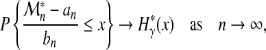
Aim. We address, here, the last-mentioned point. The issue is to decide whether or not the threading score we obtained, when aligning a given query sequence onto a fold, can be considered as an evidence that the query structure belongs to that fold. For this purpose, we need to determine what is the score probability distribution when the query sequence has no relationship with the fold it is forced to align with.
The statistical significance of threading scores is still an unsolved question and, we are aware of only a few studies tackling this problem (Bryant and Altschul, 1995; Minry et al., 2000; Panchenko et al., 1999 2000). Here, we aim at deriving a statistical significance of threading scores, based on extreme-value distributions.
2. Theoretical Framework
2.1. Problem formalization
Sequence-fold alignment. Homologous proteins conserve, during evolutionary times, a “core” substructure consisting of important structural parts such as α-helices, β-strands, turns, or functional regions such as active sites, dispersed throughout the sequence (Chothia and Lesk, 1986). Such conserved blocks and their mutual arrangement constitute the basis of any classification of structures as folds.
A fold is therefore a class of protein structures, or domain structures, which share a similar architecture. For the purpose of threading methods, it is described in a way which makes it generic and representative of all the class, as a mandatory series of blocks connected by loops whose lengths and compositions are expected to vary. A major ingredient of this description is the contact map, a graph whose vertices are the amino-acids of the blocks and where edges join amino-acids in close contact in the fold (Fig. 1).
FIG. 1.

Contact map: the fold is represented by ordered blocks. Edges join amino acid pairs brought in contact by the fold. The query sequence (red line) passes through the blocks (blue boxes) without indels, but distances between blocks are not fixed. A substitution function gives the cost of replacing amino acid pairs in contact: e.g., (H E) by (A M).
The alignment of a sequence onto a fold consists of the alignment of successive sequence segments with the blocks of the fold, in the same order. Details, without consequences for our purpose, depend on the threading method. Some methods allow blocks to be skipped. As distances between blocks are not fixed, there is usually a huge number of different alignments of a given sequence onto a given fold.
Let  be a sequence on the finite alphabet of amino-acids
  , and C be a given fold containing m blocks,
  , each of length
  . An alignment I of the sequence A onto the fold C is defined by the terms of A which start each block. Let
  be the corresponding indices. Each choice of m indices such that i1 > 0, i2 ≥ i1 + l1,
  and im + lm ≤ n, defines a specific alignment, and all alignments can be characterized in this way.
Score. The score associated with a given alignment of the query onto a fold, is a sum of terms which depend on the amino-acid pairs brought in contact by the alignment (Fig. 1). The exact definition of these terms depends on the precise threading method under consideration, without much importance for our purpose; usually, these terms also depend on the local environment (e.g., surface exposed or buried positions in the 3D structure). Threading methods can take into account the substitution cost of a residue pair in contact in the native structure by a new one, or the energetic cost of placing two amino acids at particular sites in the structure, with a characteristic structural environment, or both (Bryant and Altschul, 1995).
Let  be 1 if sites (j, k) and (j′, k′) are joined by an edge in the contact map, and 0 otherwise (the site (j, k) is the position k + 1 in block j). The score of an alignment I is typically defined as
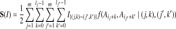 |
a sum of terms each representing the cost of placing amino-acids  and
and  in contact, in the context defined by the sites (j, k) and (j′, k′).
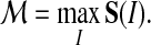
Different alignments have correlated scores, especially if they share common subalignments of blocks. The threading score  is the maximum of all these scores
 |
(1) |
Finding out, in a reasonnable time, the optimal alignment, and thus the threading score, is a hard problem which will not be developed here. Very satisfactory algorithms were developed (Andonov et al., 2008).
Global and semi-global alignments. A fold is the substructure common to several similar structures. These structures correspond to proteins or domains of similar lengths ; they are represented by the same template.
When the query sequence has a length (n) similar to that of the fold, the latter may represent its 3D structure. The whole sequence is aligned with the fold: all possible alignments are admissible. This is called a global alignment problem.
On the other hand, when the query sequence is much longer than the fold, this one may only be a structural domain. The alignment makes sense only if it extends in a region whose length is of the order of that of the fold. Therefore, admissible alignments, those to be taken into account, must not extend beyond a maximum length, say lmax. This is called a semi-global alignment problem. Only alignments such that im + lm − i1 ≤ lmax are admissible.
This constraint is active only in the semi-global regime (n > lmax), and the global alignment problem can be formally considered as a semi-global alignment problem with n ≤ lmax.
Threading score as an extreme value. The threading score of a query sequence with respect to a given fold is the largest score among all admissible alignments of that sequence onto that fold:
• If the fold under consideration corresponds to the structure of the query sequence (hypothesis H1), hopefully, a large threading score is expected.
• On the contrary, if the query sequence native structure is unrelated to the fold under consideration (hypothesis H0) we can consider the threading score, as the maximun of a set of dependent random values. This leads us to consider, under hypothesis H0, threading scores as extreme values.
2.2. Extreme value distribution
Extreme value of a sample. Extreme value theory has been first developed for sets of independent identically distributed (i.i.d.) random variables.
Let 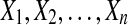 be a sequence of i.i.d real random variables with cumulative distribution function (CDF) F and
 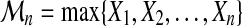 . The cumulative distribution of
  is simply derived as
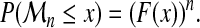 |
(2) |
However, if F ( · ) is unknown, this is not helpful in practice. The limit of  , as n tends to infinity, is either 0, if F(x) < 1, or 1 if F(x) = 1. This limit is somewhat trivial and too crude. Extreme Value Theory has been developed to understand how
 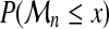 tends to 0, ∀x : F(x) < 1. Obviously, some normalization is needed.
Fréchet (1927), Fisher and Tippett (1928), and Gnedenko (1943) proved that under general asumptions on F, there exist two series an and bn and a constant γ such that:
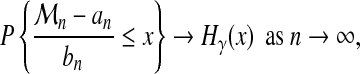 |
(3) |
with the cumulative distribution function
 |
(4) |
where y+ = max(0, y). So we have for n large enough
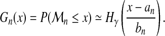 |
(5) |
According to the value of γ (positive, zero, negative), there are three families of extreme value distributions, referred to as Fréchet, Gumbel, and Weibull, respectively. Fréchet is the extreme value distribution for heavy tailed distributions, Gumbel for light tailed distributions, and Weibull for distributions with bounded tail. There is no other limit distribution than those of equation (4), but not all distributions lead to such extreme value distributions (de Haan and Ferreira, 2006). In particular, discrete distributions do not fit these distributions, their limits are degenerate.
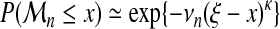
For reasons explained later on, we will be here mostly concerned with the third family, i.e., Weibull. Hence, since γ < 0, equation (5) can be rewritten as follows:
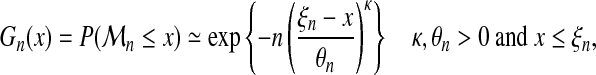 |
(6) |
where κ = − 1/γ, θn = −n−γbn/γ and ξn = an − bn/γ.
Limits for large samples. Consider a sample of size nm. Applying (6) we have:
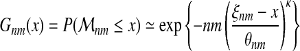 |
With equation (2), we also have the following approximation:
 |
Indeed, for probability distributions with bounded tail, provided there exists a convergence toward a Weibull type extreme value distribution, parameters θn and ξn in equation (6) converge as n → ∞ toward finite limits θ∞ > 0 and ξ∞ (the latter is the upper bound of the support of F; it is often written as F−1(1)) (de Haan and Ferreira, 2006).
Extreme value of a process. Extreme-value theory has been extended to dependent variables, particularly stationary processes. A theorem is of great value for our problem (Coles, 2003).
Consider a stationary process  , and a sample of independent variables
  with the same marginal distribution (
 has the same distribution as Xi).
Define  , and
, and 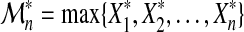 . Provided there are two sequences {bn > 0} and {an} such that, as in (3)
 |
then, under general mixing hypotheses on process X (distant events become nearly independent),
 |
where
 |
(7) |
for some constant 0 ≤ η ≤ 1. Parameters {an}, {bn} and γ are the same. Using (6), we get
 |
(8) |
nη is the effective size of the process. By reparameterizing (8), we have
 |
(9) |
with  , the scaled effective size of the process.
Parameter estimation. Much of the litterature devoted to parameter estimation in extreme value theory deals with chronological series. Estimation consists in exploiting, in such series, the distribution of very large values, or the distribution of excesses above a given threshold, to build estimates. We face a much simpler problem since, as will be seen later, we can simulate samples of extreme values.
We selected two methods for the estimation of the three parameters κ, ξn and νn in equation (9) from a sample of size m of extreme values  :
:
• Maximum likelihood estimation (MLE)
• Probability-weighted moment estimation (PWM)
The latter will be briefly exposed now (Hosking et al., 1985). The rth probability-weighted moment of  is defined as
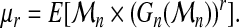 |
(10) |
A straightforward calculation with equation (6) leads to:
 |
(11) |
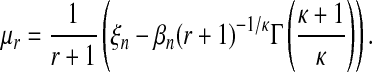
with 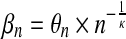 and Γ() the Gamma function. The following relations hold:
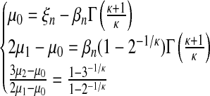 |
(12) |
Parameters are estimated by solving equations (12) where moments are replaced by their estimations, say  for μr. Estimator
  is itself obtained by replacing, in the definition (10), the expectation by the sample mean and G by the empirical cumulative distribution function of the sample
  .
.
 |
where  stands for the ith observation in the ordered sample.
2.3. Threading scores of random sequences
As explained before, threading scores under the null hypothesis will be compared to the distribution of the threading score of a random sequence. These random sequences have to be simulated under some suitable stationary mixing model, for instance a Markov model or even a sequence of independent amino acids.
Global threading score. Due to a rich combinatorics, the number of alignments of a query onto a fold increases more than exponentially fast with the length of the query. Let 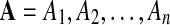 be a simulated protein sequence and C a fold. As the sequence A is a stochastic process (of amino-acids), the scores of all admissible alignments constitute a set of dependent random variables. As scores are upper bounded, we can expect that the global threading score,
  , approximately follows a Weibull type extreme value distribution as given by equation (9).
Semi-global threading score for large sequences. Alignments of A onto C can be classified according to their last position: class  contains all the alignments ending at position i (Fig. 2). Classes
  , which exist in a semi-global alignment problem (n > lmax) have all the same number of elements, since for two such classes
  and
and  , translation by i − j is a bijection. Beyond lmax, the number of admissible alignments increases linearly with n. Classes
  are incomplete, since their elements are limited in their extension to the left.
FIG. 2.

Classification of the alignments by their end. Admissible alignments of class  cannot extend out of the double arrow ending at i, of length ≤ lmax. The largest score
 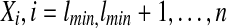 , is associated to each class.
At each class  , we can associate Xi, the highest score of all alignments of
  . The threading score
  of A with respect to C obviously verifies:
 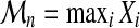 .
.
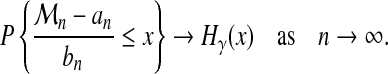
Since A is stationnary and mixing,  , is also stationnary and mixing. Suppose Xi, i ≥ lmax, follows approximately a Weibull type extreme value distribution as in equation (9) with n = lmax. As the process {Xi, i ≥ lmax} verifies the conditions of the theorem on extreme value distribution of a stationnary process, we can apply equation (7). It follows that, for large n,
  has approximately a Weibull type extreme value distribution:
 |
for some 0 ≤ η ≤ 1. Since  and κ are unknown and must be estimated, this equation must be rewritten:
 |
(13) |
for some parameters λ1 > 0, κ > 0, and with ξmax > x
Now the threading score can be written as 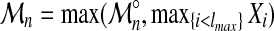 .
.
Term  , contributes to
  only if it is larger than
  , hence in the very tail of its distribution, where it can be approximated by a distribution of type (6) for some ficticious size N0. Using the convergence exposed before, we can approximate the parameter
  by
by  . It finally turns out, if all this story holds, that the contribution of this last term consists in increasing by a constant, the scaled effective size.
We finally can predict, for very large sequence sizes (n >> lmax), the following distribution of the threading score  :
:
 |
(14) |
The dependence of the threading score cumulative distribution function, Gn(x), on sequence length, is asymptotically localized in the parameter νn, with an affine form.
Otherwise, for all sequence sizes, the threading score  should have a distribution of the form (9).
3. Results and Discussion
Simulations were carried out to test these predictions, to demonstrate the existence of a suitable distribution for the threading score of a random sequence, and to validate a parameter estimation procedure. Of course, these parameter values depend on the precise threading method used and on the random sequence simulation model. They must be reestimated each time these choices are changed.
3.1. Numerical experiment
3.1.1. Experimental design
Folds. Two folds were chosen, 1bjaA and 1gtvA. Native sequences have 95 and 214 residues. Fold 1bjaA (respectively, 1gtvA) has lmin = 87 (respectively, lmin = 181), and we set lmax = 110 (respectively, lmax = 226).
Sequence simulation. Sequences were simulated as independent series of amino acids, using a published probability distribution (Robinson and Robinson, 1991) (Table 1). This simple model can be criticized as an unrealistic protein sequence representation, but we use it here only as a way to generate random threading scores, and, as will be discussed later, it seems to have little consequences on the final distribution.
Table 1.
Probabilities Used for Amino Acid Random Sequence Simulation
| π(A) = 0.0781 | π(C) = 0.0192 | π(D) = 0.0537 | π(E) = 0.0629 | π(F) = 0.0385 |
| π(G) = 0.0738 | π(H) = 0.0220 | π(I) = 0.0514 | π(K) = 0.0574 | π(L) = 0.0903 |
| π(M) = 0.0224 | π(N) = 0.0449 | π(P) = 0.0520 | π(Q) = 0.0426 | π(R) = 0.0513 |
| π(S) = 0.0712 | π(T) = 0.0584 | π(V) = 0.0644 | π(W) = 0.0133 | π(Y) = 0.0322 |
For each fold, 11 sequence lengths were chosen:
• 1bjaA: 90, 97, 105, 115, 124, 143, 170, 190, 200, 350 and 500.
• 1gtvA: 184, 193, 220, 250, 279, 321, 350, 400, 430, 500 and 610.
These samples covered the global and semi-global regimes, depending on whether the sequence length is shorter or longer than lmax.
For each pair {fold × length}, a sample set of 6,000 sequences was generated.
FROST (Fold Recognition-Oriented Search Tool). FROST is the threading method we used here to calculate the threading scores of each of these simulated sequences, thus providing samples of independent threading scores. FROST has been shown more efficient than methods like PSI-BLAST and 3D-PSSM for the detection of remote homologs (Marin et al., 2002).
FROST uses a 3D substitution function which corresponds to the cost of replacing a given pair of residues, in contact in the structure, by one belonging to the query. This cost takes into account environmental factors such as the localization in the 3 structure (buried or exposed sites, type of secondary structure) (Marin et al., 2002). In the 3D function, no gap penalty is used. The score depends on structure and query sequence. Given a structure and query length, the highest it is, the most reliable is the fold prediction.
3.1.2. Choosing an extreme-value distribution model
Both folds were treated separately. Four different models will be compared, named A, B, C, D. For each sequence length, n, each model associates a Weibull type extreme-value distribution. They differ by constraints set on parameters, according to the following equations:
- Model A: no constraint on parameters,

(15) - Model B: common κ, see equation (9),

(16) - Model C: common κ and ξ, see “limits for large samples,”
(17) - Model D: common κ and ξ, νn affine function of n, see equation (14),

(18)
They verify the following inclusion relations: A ⊃ B ⊃ C ⊃ D.
To test a submodel, a usual procedure relies on maximum likelihood ratio. We did not follow this procedure since our estimation procedure did not always rely on likelihood maximization. We based our model choice procedure on Kolmogorov-Smirnov test statistics. Under the null hypothesis, p-values are uniformly distributed on [0, 1]: small p-values indicate a poor fit. Being non-parametric, this test is very robust but it is also very powerful.
Model A: testing the extreme-value distribution. An extreme-value distribution defined by equation (15) is fitted separately to each sample. This model is a generalization of equation (9), since κ depends on n.
Parameters were estimated by probability weighted moment, PWM (Fig. 3) and by maximum likelihood, MLE, with very similar results (Fig. 4). PWM has the advantage to be direct, when MLE is iterative.
FIG. 3.

Model A. Probability-weighed moments (left) and functions of them (right) used in parameter estimation (equations (12)) for both folds 1bjaA (upper figures) and 1gtvA (lower figures).
FIG. 4.

Model A. Empirical and adjusted threading score CDF according to different sequence lengths (as indicated on the curves) for both folds 1bjaA (left) and 1gtvA (right). Extreme-value distribution parameters of model A are estimated for each sample by PWM (upper) and MLE (lower).
Estimations and goodness-of-fit tests are displayed in Table 2 for PWM. Parameter γ of equation (5) was found in all samples highly significantly negative (remember  ) and Kolmogorov-Smirnov test indicated an excellent adjustment. This confirms that threading score distribution of random sequences can be very well approximated by a Weibull type extreme-value distribution. Therefore, cumulative distribution functions will hereafter always be presented in the form of equation (9).
Table 2.
Model A: For Each Fold and Length Separately, Parameters Are Estimated by PWM; Kolmogorov-Smirnov Test p-Values Are Also Shown
|
1bjaA |
1gtvA |
||||||||
|---|---|---|---|---|---|---|---|---|---|
| Length n | κn | ξn | βn | K-S p-value | Length n | κn | ξn | βn | K-S p-value |
| 90 | 3.91 | −3.98 | 25.77 | 0.37 | 184 | 4.17 | −28.34 | 39.43 | 0.37 |
| 97 | 3.96 | 5.06 | 24.26 | 0.61 | 193 | 4.41 | −6.14 | 37.82 | 0.82 |
| 105 | 4.21 | 11.23 | 24.20 | 0.46 | 220 | 4.71 | 21.96 | 38.89 | 0.86 |
| 115 | 4.61 | 17.02 | 24.89 | 0.69 | 250 | 4.70 | 32.94 | 35.42 | 0.41 |
| 124 | 4.75 | 19.76 | 24.16 | 0.25 | 279 | 4.80 | 42.91 | 36.40 | 0.67 |
| 143 | 4.52 | 22.47 | 22.12 | 0.26 | 321 | 4.50 | 48.63 | 32.79 | 0.46 |
| 170 | 4.66 | 26.61 | 21.92 | 0.56 | 350 | 4.81 | 56.51 | 35.82 | 0.88 |
| 190 | 4.93 | 29.96 | 22.78 | 0.78 | 400 | 4.82 | 59.72 | 32.59 | 0.82 |
| 200 | 4.39 | 28.03 | 19.76 | 0.56 | 430 | 4.43 | 60.60 | 30.24 | 0.60 |
| 350 | 5.21 | 33.02 | 18.95 | 0.39 | 500 | 5.17 | 65.85 | 31.58 | 0.58 |
| 500 | 5.35 | 33.85 | 17.88 | 0.74 | 610 | 5.35 | 68.81 | 31.54 | 0.92 |
Increasing the sequence length causes almost monotonous changes in all parameters. κn increases (but not significantly as will soon be seen), while  decreases, and ξn increases very much. This is not surprising for βn. Concerning ξn, we would expect a convergence toward an upper value ξ∞. The output on κn is more unexpected. But the large correlation between estimators (not shown here) hinders a detailed interpretation and certainly explains the observed apparent irregularities in the parameter evolution with sequence length.
Model B: testing a common form parameter κ. We then fitted these distributions under model B, equation (16), where κ is common, which corresponds exactly to equation (9). Figure 5 displays the empirical and fitted CDF, parameters estimated by PWM. When using PWM estimation procedure, we first estimated κ by solving a derivation of the third equation in (12) where L is the set of sampled sequence lengths, and  the estimated rth weighted moment for sequence length n:
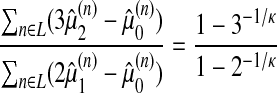
FIG. 5.

Model B. Empirical and adjusted threading score CDF according to different sequence lengths (as in Fig. 4) for both folds 1bjaA (left) and 1gtvA (right). Extreme-value distribution parameters of model B are estimated for each fold by PWM.
Table 3 displays parameter estimations and Kolmogorov-Smirnov test p-values. It turns out that model B provides a very satisfactory approximation of the threading score distribution of a random sequence, in agreement with the prevision made.
Table 3.
Model B: For Each Fold, Parameters κco (Common) ξn and βn Are Estimated by PWM; Kolmogrov-Smirnov Test p-Values Are Also Shown
|
1bjaA |
1gtvA |
||||||||
|---|---|---|---|---|---|---|---|---|---|
| Length n | κco | ξn | βn | K-S p-value | Length n | κco | ξn | βn | K-S p-value |
| 90 | 4.58 | −0.43 | 29.61 | 0.26 | 184 | 4.91 | −22.49 | 45.56 | 0.38 |
| 97 | 7.73 | 27.26 | 0.72 | 193 | −2.02 | 41.98 | 0.77 | ||
| 105 | 12.25 | 25.26 | 0.20 | 220 | 22.12 | 38.94 | 0.87 | ||
| 115 | 16.89 | 24.88 | 0.50 | 250 | 34.98 | 37.37 | 0.36 | ||
| 124 | 18.97 | 23.50 | 0.26 | 279 | 43.31 | 36.80 | 0.87 | ||
| 143 | 22.82 | 22.54 | 0.29 | 321 | 51.21 | 35.74 | 0.46 | ||
| 170 | 26.30 | 21.46 | 0.59 | 350 | 56.27 | 35.60 | 0.94 | ||
| 190 | 28.26 | 21.03 | 0.77 | 400 | 60.84 | 33.81 | 0.82 | ||
| 200 | 29.03 | 20.75 | 0.59 | 430 | 63.47 | 33.36 | 0.57 | ||
| 350 | 31.44 | 17.40 | 0.41 | 500 | 65.50 | 31.23 | 0.41 | ||
| 500 | 31.95 | 15.96 | 0.09 | 610 | 66.35 | 28.88 | 0.36 | ||
In model B,  increases with n, while
  decreases, in a much more regular way as in model A: owing to the constraint on κ, estimator correlations are much smaller, and estimation more stable. Figure 6 displays, for all values of the sequence length n, νn and ξn, as estimated in model B. For large values of n, θn and ξn almost converged, while νn varies linearly, which corresponds to the expected convergence for large sequences, and leads to model D.
FIG. 6.

Model B. 1bjaA (left) and 1gtvA (right);  and ξn defined by equation (9); κco common, νn tends to vary linearly while ξn “numerically converges,” as n becomes very large.
Models C and D: testing an asymptotic distribution for large sequences. We then fitted these distributions under model C (equation (17)), where κ and ξ are common. Results show without doubt that this model is unacceptable on the whole range of sequence lengths (Fig. 7).
FIG. 7.

Model C. Empirical and adjusted threading score CDF, according to sequence length (indicated on the curves) for both folds 1bjaA (left) and 1gtvA (right). Parameters are estimated by MLE.
We then tried to find out if the longest sequences (n > n′ for some n′) could be fitted to model D, defined by equation (18). We first estimated n′ by testing the maximum number of longest sequences for which model C would be acceptable. We then computed the linear regression of νn on n for n > n′.
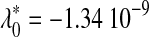
Table 4 displays, for each fold, estimations and goodness-of-fit statistics for the highest sets of long sequences for which model C is acceptable. Relative to each fold, n′ is approximately twice lmax (n′ = 190 for fold 1bjaA, and n′ = 430 for fold 1gtvA). Coefficients of the linear regression of νn on n (equation 14) are at the bottom of Table 4. Parameter  is positive in both cases, in agreement with the prediction made previously, where λ0 had been interpreted as a ficticious sample size, thus should be positive. However, this interpretation must be considered carefully, since it relies on the assumption, ξ constant over the whole range of sequence lengths, which is not verified here; ξ converges as n increases, but is significantly less for short sequences; that is why model C is rejected for short sequences.
Table 4.
Model D: For Each Fold a Common ξco and κco Are Computed (Model C) for “Long” Sequences Only
|
1bjaA |
1gtvA |
||||||||
|---|---|---|---|---|---|---|---|---|---|
| Leng. | κco | ξco | βn | K-S p-val. | Leng. | κco | ξco | βn | K-S p-val. |
| 190 | 6.07 | 35.86 | 28.69 | 0.25 | 430 | 5.64 | 69.47 | 39.25 | 0.36 |
| 200 | — | — | 27.72 | 0.16 | 500 | — | — | 35.24 | 0.55 |
| 350 | — | — | 21.88 | 0.25 | 610 | — | — | 32.19 | 0.66 |
| 500 | — | — | 19.97 | 0.54 | |||||
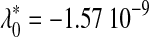 λ1 = 3.18 10−11 λ1 = 3.18 10−11
|
p = 1.7 10−5 |
 λ1 = 1.20 10−11 λ1 = 1.20 10−11
|
p = 0.01 | ||||||
Kolmogorov-Smirnov goodness-of-fit test is carried out. Bottom,  and
and  are the parameters of the linear regression of
  on sequence length n; see equation (14). p-Value of the linear regression model is presented.
3.1.3. Parameter interpolation/smoothing
According to previous sections, we propose to compute a p-value on the basis of model B if n ≤ n′ (global and non-asymptotic semi-global regimes) and model D if n > n′ (asymptotic semi-global regime). In practical situations, these distributions must be used with parameter values corresponding to the exact query length.
In the asymptotic regime (n > n′), model D provides an explicit value for all parameters.
In the non-asymptotic regime (n ≤ n′), parameters of model B can be precalculated at sampled lengths and further estimated at the exact length n of the query by interpolation or smoothing.
We present some adjustments obtained with parameters calculated for the exact length after interpolation of the estimated weighted moments. Results are satisfactory. This point will not be further developed here.
Global and non-asymptotic semi-global regimes. We generated random sequence samples of 10 (fold 1bjaA) and nine (fold 1gtvA) different lengths, covering all the range of global and semi-global regimes. Threading score distributions were computed with model B whose parameters, ξn and βn, were estimated after interpolation of the weighted moments (Fig. 8).
FIG. 8.

Prediction with model B for medium-length sequences in the non-asymptotic semi-global regime. κco equals 4.62 for 1bjaA (upper) and 4.85 for 1gtvA (lower) ; ξn and νn are calculated from interpolated weighted moments. The range covers the non-asymptotic semi-global regime and its boundaries.
Asymptotic semi-global regime. Model D solves the problem of p-value calculations for very long sequences in the semi-global regime, with explicit parameter values. To check the prediction quality, two samples of 6,000 sequences of different lengths (600 and 1000 for 1bjaA, 750 and 1000 for 1gtvA) were generated and the predicted distribution of their threading scores computed with the parameters shown in Table 4, and compared to the empirical distribution. Kolmogorov-Smirnov test p-values are 0.16 and 0.05 for lengths 600 and 1000 with 1bjaA, and 0.06 and 0.07 for lengths 750 and 1000 with 1gtvA (Fig. 9).
FIG. 9.

Prediction with model D for long sequences. The first two curves refer to comparison among sequences of lengths 600 and 1000 (fold 1bjaA). The second two curves to comparison among sequences of lengths 750 and 1000 (fold 1gtvA).
3.2. Threading scores of real protein sequences
So far we found a suitable representation of the threading score distribution of random sequences. The problem addressed here, consists in studying the score distribution of real protein sequences, whether their structures are alien, or on the contrary do belong, to the fold under consideration.
The problem is in fact complex, since homolog proteins are more or less related: hypothesis H1 is composite. The way in which structural similarity is handled and its consequences on the threading score, strongly depends on the precise threading method considered, as will be discussed later. Thus, a precise discussion of these distributions is far beyond the scope of this article. In order to illustrate this point, we will just examine results obtained with a reduced set of sequences.
SCOP database. The SCOP database (Murzin et al., 1995), is a widely used protein classification in which most proteins of known structures are sorted in a hierarchical way. It constitutes a tool to build sets of more or less structurally related sequences.
SCOP clusters homologous proteins into families. Most families group proteins sharing at least 30% residue identity.
SCOP clusters families into superfamilies if their proteins are structurally and functionally similar.
3.2.1. Threading different sequences onto a fold
Data. Four sets of real protein sequences were constituted representing different similarity classes with respect to the structure of 1gtvA.
The first set (“psi-blast homologs”) consists of proteins collected via psi-blast, thus sharing a significant sequence similarity with 1gtvA. Their structure is unknown, but almost certainly similar to that of 1gtvA, owing to the clear sequence similarity.
The next three sets are disjoint and their structures are experimentally known.
The second set (“SCOP family”) contains all proteins belonging to the same SCOP family as 1gtvA. These proteins share a structural and functional similarity with 1gtvA, and are certainly homologous.
The third set (“SCOP superfamily”) contains all proteins belonging to the same SCOP superfamily than 1gtvA, but to a different family. These proteins present only a moderate sequence similarity with 1gtvA, less than 20% sequence identity, although they are structurally related.
The fourth set (“other SCOP folds”) collects proteins belonging to other folds, thus presenting no structural similarity with 1gtvA, and less than 20% sequence identity with 1gtvA. These are in fact 44 “alpha-beta” protein sequences of length lying between 187 and 226, thus belonging to the “global regime.”
VAST. For the last three sets, for which structures are known, structural similarity of each protein with 1gtvA was quantified, using VAST (Madej et al., 1995), a structure alignment program. This program optimally superimposes the residues of a protein onto the residues of the other one. The number of residue pairs successfully superimposed by VAST is expressed as a proportion of the number of residues of the smallest protein.
Results. Threading scores obtained with these sets of sequences are displayed in Figure 10. These results will be discussed later.
FIG. 10.

Histograms of p-values under null hypothesis. Upper left: 1gtvA psi-blast 600 nearest homologs. Lower left: SCOP family of 1gtvA. Lower right: SCOP superfamily of 1gtvA, but other families. Upper right: other SCOP folds than that of 1gtvA. p-values were computed using model B.
Psi-blast homologs are close homologs, and very small p-values are expected. Most p-values are small, but a non negligible proportion is higher than expected (upper left graph).
Sequences of the SCOP family of 1gtvA, display, as expected, more dispersed p-values than psi-blast homologs (lower left). Only a small proportion of these p-values is small enough to point a structural similarity.
Sequences belonging to other families of the SCOP superfamily of 1gtvA, display, as expected, even more dispersed, but still not uniformly distributed, p-values (lower right).
Sequences belonging to other SCOP superfamilies than 1gtvA, display a p-value histogram compatible with the expected uniform distribution (upper right).
3.2.2. Threading a sequence onto different folds
A sequence of 260 residues, the native sequence of 1k77A, was aligned on four different folds 1i60A, 1qtwA, 1qpoA, and 1m40A of length 212, 189, 243, and 200, respectively. These folds had been previously sorted from structurally close to structurally very far from 1k77A (Taly et al., 2008; Grelaud et al., 2009). Sequence and structure similarity indicators are displayed in Table 5.
Table 5.
Comparison of 1k77A to Four Different Proteins
| |
Adjusted EVD Param. |
|
|
|
|
|
||
|---|---|---|---|---|---|---|---|---|
| Fold | κ | ξ | β | K-S p-value | Sequence ident. (%) | Structural simil. (%) | rmsd (Å) | Threading score p-value |
| 1i60A | 4.45 | −24.67 | 45.68 | 0.15 | 18.6 | 93.1 | 2.97 | 0.07 |
| 1qtwA | 4.62 | 31.7 | 33.76 | 0.14 | 12.1 | 91.9 | 3.35 | 0.26 |
| 1qpoA | 4.31 | −47.5 | 45.72 | 0.43 | 7.6 | 50.8 | 3.37 | 0.73 |
| 1m40A | 4.31 | 23.46 | 47.15 | 0.09 | 3.6 | 10.7 | 3.02 | 0.79 |
Four first colomns refer to the calculated extreme value distribution of random sequence threading scores. Proteins were selected to exhibit different levels of structure and sequence similarities with 1k77A: 1i60A and 1qtwA belong to its SCOP superfamily, 1qpoA to its fold, and 1m40A to a different, structurally unrelated, class. Threading score p-values were calculated with adjusted extreme-value distributions.
Threading score distributions of random sequences had to be estimated for each fold. 20,000 sequences of length 260 were independently generated and estimation carried out by PWM method, using model A. As indicated by the Kolmogorov-Smirnov p-values, the fitted extreme value distributions on simulated data are acceptable (Table 5).
Table 5 also displays threading score p-values, computed with the fitted distributions, of the native sequence of 1k77A, when folded on each of these four different folds. These p-values are in total agreement with structural similarities between the native fold of the query and each of the four different folds. It is worth noticing that only the first p-value, obtained when folding 1k77A onto 1i60A, is small enough to detect a structural similarity at a significance level of 10%. Other structures do not display p-values small enough to be detected as significant at any reasonnable level.
4. Discussion
Previous sections show that a Weibull type extreme value distribution can be adjusted to threading scores of random sequences, on the whole range of sequence lengths that are encountered in realistic situations, with an excellent fit. This is substantially more than just expected according to extreme value theory.
First, extreme value theory provides asymptotic results, corresponding to long sequences. Our numerical experiment shows that the results hold even for very short sequences, down to the shortest it is possible to thread on a given fold.
Second, results also hold for very long sequences, which is somewhat surprising for another reason. Threading scores are essentially discrete variables and therefore their real extreme value distributions are degenerate. One might have feared, that very long random sequences would produce degenerate extreme values. This is not the case. Score values are so numerous and well spread that the score distribution, in its central part, can be reasonably approximated by a continuous distribution. Threading scores of very long random sequences go far in the tail of the score distribution, but, due to the very strong limitation of the number of admissible alignments introduced by the semi-global regime, not far enough to reach its very tail where this continuous approximation no longer holds. Things go as if scores of random sequences, even very long ones, were continuous variables. This observation refers to random sequences, it does not hold for close homologs of the native structure, as will be discussed later.
Indeed, the set of all possible configurations of a contact map with q vertices, is of size 20q. Contact maps are heterogeneous graphs, and the score terms attached to the edges depend on the local environment, so that there are almost as much different possible score values building the score set. On the other hand, the optimization set, the set of scores of all the admissible alignments of a given sequence (whose maximum is its threading score) is a subset of the former, with a number of elements many orders of magnitude smaller. For the fold 1bjaA (respectively 1gtvA), in the global regime with sequences of length lmax the score set is (roughly) of size 1071 (respectively 10143) when the optimization set is of size 1011 (respectively 1023). Even if the exceptionnally high score values of native related sequences are numerous, they build a set of so tiny probability that it cannot, in practice, be reached by random sequences.
Third and finally, the good agreement with a Weibull type EVD of constant form parameter κ (model A not better than model B) is also informative. The score of a random sequence is a sum of numerous terms, and naïvely, one could have expected that a Gaussian truncated at the highest possible score value would be a sufficient approximation of its distribution. But in our experiment with samples of size 6000, this highest possible value was never reached, by far, by random sequence threading scores. Thus, we could not have distinguished our samples from those obtained supposing a non truncated Gaussian score distribution. Gaussian distributions belong to the Gumbel attraction bassin, and we would have found a Gumbel EVD approximation for the threading score distribution. On the contrary, our numerical experiment tells us that the continuous approximation of the score value distribution of random sequences belongs to the Weibull attraction bassin, thus has the corresponding type of tail. The tail drops down much faster than does that of a Gaussian. This is due to the complex correlation structure of all score terms, and is much related to the properties of the contact map.
To make this point clear, let us consider an artificial example. Consider the catenary graph, where the pairs of neighbours are the pairs of successive amino-acids in the sequence. The score of a sequence alignment on this artificial structure, is a sum of elementary terms, each attached to a pair of successive amino-acids. If the sequence is random, as we simulated ours, the sequence of random elementary terms is a strongly mixing process (non-adjacent terms are independent). By the central limit theorem, the score of the alignment could be aproximated by a Gaussian. Thus, in this case, a Gumbel distribution would certainly provide a fair aproximation of the threading score of a random sequence. But such a graph is, by no way, the contact map of a real protein. Real contact maps have lots of edges linking amino-acids distant in the sequence, which are the expression of the forces that make the structure. From a probabilistic point-of-view, these distant contacts are responsible for complex correlations among the elementary terms which build up the score, and make its distribution decrease faster than that of a Gaussian.
The good agreement with a Weibull EVD certainly does not depend on the random sequence model. Provided the latter is a mixing and stationnary process, quite reasonable assumptions in fact, the same theory can be applied with certainly the same qualitative results, although with different parameters.
We generated our random sequences as series of independent random amino acids. This is very simple and quite unrealistic, and could explain part of the less appealing results observed with real sequences. Real sequences always have special features, as secondary structures, which our random sequences lack. A helix, for instance, will probably better fit another helix than a random sequence will do. Threading a real protein sequence alien to the fold, will probably often result in an alignment of several helices on helices and strands on strands, thus leading to a higher threading score than obtained with a random sequence of the same length. This could partly explain the p-value distribution obtained with the set of sequences belonging to the same superfamily, but to other families than 1gtv. We expected a distribution closer to the uniform one. Instead of being uniform, it favours small values and clearly disfavours large p-values. Anyway, this phenomenon does not seem to have very important effects on clearly unrelated sequences. Nevertheless, when implementing p-value calculation for a threading method, more realistic random sequence models would be recommanded. An interesting alternative could be Hidden Markov Models, where hidden states would represent secondary structures, emitting amino-acids with specific distributions.
Some close homologs and most remote homologs have larger p-values than expected. This is much related to the threading method used. FROST is designed in such a way that an admissible alignment of a sequence onto a fold must go through each block. Remote homologs may share strong similar parts, but some secondary structure elements, seen by FROST as blocks, can be present in a protein and absent in another one. This can completely disturb the rest of the alignment, making impossible to align the most similar parts, thus leading to a poor threading score and a large p-value.
Very close homologs of the native sequence of a fold generally have threading scores higher than the estimated parameter ξ, the highest theoretically possible value, thus leading to an undefined p-value. We never encountered, by far, such exceedingly high scores with random sequences. Close homologs have threading scores belonging to the very few highest possible values; these values reach the real threading score extreme value distribution, which, due to the discrete nature of the score, is degenerate. We are out of the domain where a continuous approximation of the score distribution is still admissible. In practical terms, this is not a problem since it points a very strong similarity, and the p-value can be conventionally set to zero.
5. Conclusion
We claim that threading score significance can be assessed using the procedure we presented in this article—that is, by comparison with the threading score distribution of a random sequence of amino acids. Parameters of this reference distribution of course depend on the length of the query, on the fold under consideration, on the threading method it is designed for, and also on the protein simulation model used (and we recommand to use something more realistic than we did).
But Weibull extreme value distributions (model B) should be suitable in any case. This result is related to properties of the contact map, and does not depend on technical details. This should hold as long as the threading score is a sum of terms, each attached to a pair of amino acids put in contact by the fold.
In practical terms, a suitable distribution is obtained with model B for short sequences and its submodel D for long sequences. For each fold, parameters can be estimated, once and off line, on a finite sample of lengths. Later on, parameters can be interpolated or extrapolated at the exact length of any query, providing immediately its threading score p-value.
Acknowledgments
We are grateful to the INRA MIGALE Bioinformatics Platform (http://migale.jouy.inra.fr) for their help and computational resources. This research was supported by the French Agence Nationale de la Recherche (grant ANR-06-CIS-008 project, PROTEUS [Calcul intensif et simulation]).
Disclosure Statement
No competing financial interests exist.
References
- Andonov R. Collet G. Gibrat J., et al. Recent advances in solving the protein threading problem. In: Talbi E.-G., editor; Zomaya A., editor. Grids for Bioinformatics and Computational Biology. Wiley-Interscience; New York: 2008. [Google Scholar]
- Box G.E.P. Cox D.R. An analysis of transformations. J. R. Stat. Soc. Ser. B. 1964;26:211–252. [Google Scholar]
- Bradley P. Misura K. Baker D. Toward high-resolution de novo structure prediction for small proteins. Science. 2005;309:1868–1871. doi: 10.1126/science.1113801. [DOI] [PubMed] [Google Scholar]
- Bryant S. Altschul S. Statistics of sequence-structure threading. Curr. Opin. Struct. Biol. 1995;5:236–244. doi: 10.1016/0959-440x(95)80082-4. [DOI] [PubMed] [Google Scholar]
- Chothia C. One thousand families for the molecular biologist. Nature. 1992;357:543–544. doi: 10.1038/357543a0. [DOI] [PubMed] [Google Scholar]
- Chothia C. Lesk A. The relation between the divergence of sequence and structure in protein. EMBO J. 1986;5:823–826. doi: 10.1002/j.1460-2075.1986.tb04288.x. [DOI] [PMC free article] [PubMed] [Google Scholar]
- Coles S. An Introduction to Statistical Modeling of Extreme Values. Springer; New York: 2003. [Google Scholar]
- Duan Y. Kollman P. Pathways to a protein folding intermediate observed in a 1-microsecond simulation in aqueous solution. Science. 1998;282:740–744. doi: 10.1126/science.282.5389.740. [DOI] [PubMed] [Google Scholar]
- Fisher R. Tippett L. Limiting forms of the frequency distribution of the largest or smallest member of a sample. Proc. Cambridge Philos. Soc. 1928;24:180–190. [Google Scholar]
- Fréchet M. Sur la loi de probabilité de l'écart maximum. Ann. Soc. Math. Polon. 1927;6:93–116. [Google Scholar]
- Gnedenko B. Sur la distribution limite du terme maximum d'une série aléatoire. Ann. Math. 1943;44:423–453. [Google Scholar]
- Godzik A. Counting and classifying possible protein folds. TIBTECH. 1997;15:147–151. [Google Scholar]
- Govindarajan S. Recabarren R. Goldstein R. Estimating the total number of protein folds. Proteins. 1999;35:408–414. [PubMed] [Google Scholar]
- Grelaud A. Robert C. P. Marin J., et al. ABC likelihood-free methods for model choice in Gibbs random fields. Bayesian Anal. 2009;4:317–336. [Google Scholar]
- de Haan L. Ferreira A. Extreme Value Theory. Springer; New York: 2006. [Google Scholar]
- Hosking J. Wallis J. Wood E. Estimation of the generalized extreme-value distribution by the method of probability-weighted moments. Technometrics. 1985;27:251–261. [Google Scholar]
- Madej J. Gibrat J. Bryant S. Threading a database of protein cores. Proteins. 1995;23:356–369. doi: 10.1002/prot.340230309. [DOI] [PubMed] [Google Scholar]
- Marin A. Pothier J. Zimmermann K, et al. Frost: a filter-based fold recognition method. Proteins. 2002;49:493–509. doi: 10.1002/prot.10231. [DOI] [PubMed] [Google Scholar]
- Minry L. Finkelstein A. Shakhnovich E. Statistical significance of protein structure prediction by threading. Proc. Natl. Acad. Sci. USA. 2000;97:9978–9983. doi: 10.1073/pnas.160271197. [DOI] [PMC free article] [PubMed] [Google Scholar]
- Murzin A. Brenner S. Hubbard T., et al. SCOP: a structural classification of proteins database for the investigation of sequences and structures. J. Mol. Biol. 1995;247:536–540. doi: 10.1006/jmbi.1995.0159. [DOI] [PubMed] [Google Scholar]
- Orengo C. Jones D. Thornton J. Protein superfamilies and domain superfolds. Nature. 1994;372:631–634. doi: 10.1038/372631a0. [DOI] [PubMed] [Google Scholar]
- Panchenko A. Marchler-Bauer A. Bryant S. Threading with explicit models for evolutionary conservation of structure and sequence. Proteins. 1999;37:133–140. doi: 10.1002/(sici)1097-0134(1999)37:3+<133::aid-prot18>3.3.co;2-4. [DOI] [PubMed] [Google Scholar]
- Panchenko A. Marchler-Bauer A. Bryant S. Combination of threading potentials and sequence profiles improves fold-recognition. J. Mol. Biol. 2000;296:1319–1331. doi: 10.1006/jmbi.2000.3541. [DOI] [PubMed] [Google Scholar]
- Robinson A. Robinson L. Distribution of glutamine and asparagine residues and their near neighbors in peptides and proteins. Proc. Natl. Acad. Sci. USA. 1991;88:8880–8884. doi: 10.1073/pnas.88.20.8880. [DOI] [PMC free article] [PubMed] [Google Scholar]
- Taly J. Marin A. Gibrat J. Can molecular dynamics simulations help in discriminating correct from erroneous protein 3D models? BMC Bioinform. 2008;9:6. doi: 10.1186/1471-2105-9-6. [DOI] [PMC free article] [PubMed] [Google Scholar]
- Wang Z. How many fold types of protein are there in nature? Proteins. 1996;26:186–191. doi: 10.1002/(SICI)1097-0134(199610)26:2<186::AID-PROT8>3.0.CO;2-E. [DOI] [PubMed] [Google Scholar]
- Wang Z. A re-estimation for the total numbers of protein folds and superfamilies. Protein Eng. 1998;11:621–626. doi: 10.1093/protein/11.8.621. [DOI] [PubMed] [Google Scholar]